Munich Personal RePEc Archive
Patterns of Price Competition and the
Structure of Consumer Choice
Armstrong, Mark and Vickers, John
Department of Economics, University of Oxford
January 2020
Online at
https://mpra.ub.uni-muenchen.de/98346/
Patterns of Price Competition and the Structure of
Consumer Choice
Mark Armstrong
John Vickers
January 2020
Abstract
We explore patterns of price competition in an oligopoly where consumers vary in the set of suppliers they consider for their purchase. In the case of “nested reach” we …nd equilibria, unlike those in existing models, in which price competition is segmented: small …rms o¤er only low prices and large …rms only o¤er high prices. We characterize equilibria in the three-…rm case using correlation measures of interaction between pairs of …rms. We show how entry, merger and market expansion can a¤ect patterns of price competition in novel ways.
1
Introduction
We study oligopoly pricing in a setting where consumers di¤er in their choice sets—that is, the set of …rms they consider for their purchase—and buy from the …rm in their choice set with the lowest price. Bertrand equilibrium then involves …rms choosing their prices according to mixed strategies, and a …rm chooses from a range of prices. The structure of price competition could take many forms. Firms might all choose from a similar range of prices, or competition might be more segmented with only a small subset of …rms competing at a given price. Who competes with whom at each price is determined in equilibrium. How does the equilibrium structure of price competition depend on the underlying structure of consumer choice sets?
The simplest situation in which this question arises is a duopoly in which each …rm has some captive customers, while non-captive customers are able to pay the lower of the two
Both authors at Department of Economics and All Souls College, University of Oxford. We are grateful to Massimo De Francesco, Daisuke Hirata, Maarten Janssen, Jon Levin, Domenico Menicucci, Vlad Nora, Martin Obradovits, David Ronayne, Neri Salvadori, Robert Somogyi, and Jidong Zhou for helpful comments. Armstrong thanks the European Research Council for …nancial support from Advanced Grant 833849.
…rms’ prices. A …rm then has choice between “entering the fray”, by competing against its rival for the contested consumer segment with a low price, or “retreating” back towards its captive base by setting a high price, and in equilibrium these strategies yield the same pro…t. Even if the …rms are asymmetric, they use the same interval range of prices. With more than two …rms, though, richer patterns of consumer consideration become possible. Taking the interaction between two …rms to be the “overlap” in the sets of consumers who consider buying from them, di¤erent pairs of …rms might have very di¤erent levels of interaction. With more than one rival a …rm can compete on several fronts, and richer patterns of pricing also emerge. With a segmented pricing pattern, for instance, a …rm might compete against one …rm when it charges a low price and another …rm when it charges a higher price.
The foundation of our model is the distribution of choice sets among consumers. There are various reasons why di¤erent consumers have di¤erent sets of choices open to them. Perhaps following a prior stage of advertising by …rms or search by consumers, some con-sumers become aware of a di¤erent set of suppliers than other concon-sumers. For instance, Draganska and Klapper (2011) document limited and heterogeneous consumer awareness of various brands of ground co¤ee, while Honka, Hortacsu, and Vitorino (2017) do the same for retail banks. Alternatively, as in Spiegler (2006), there might be horizontal product di¤erentiation such that only a subset of products could meet a consumer’s needs. The set of …rms who are currently active in the market might be uncertain (Janssen and Rasmusen (2002)), as might be the set of …rms who choose to post prices on a comparison website (Baye and Morgan (2001)). Some consumers might be constrained in their choices by loca-tion, transport costs or switching costs. For instance, some models of spatial competiloca-tion, such as Smith (2004), suppose that a consumer considers buying from those …rms located within a speci…ed radius of her. Consumers might also di¤er in their ability to make com-parisons between o¤ers, with confused consumers choosing randomly between suppliers or buying from a default seller (Piccione and Spiegler (2012), Chioveanu and Zhou (2013)). Our analysis does not take a view on the underlying reason why consumers have di¤erent choice sets. Rather, it takes the distribution of choice sets in the consumer population as given, and explores the consequences for competition.
A considerable literature has explored aspects of this general framework, and some settings are now well understood: (i) the case with symmetric …rms; (ii) the case with
independent reach, and (iii) the “one-or-all” case where consumers are either captive to one …rm or can choose between all …rms. (These special cases, which overlap, are discussed in more detail in section 2.) Within case (i), which covers the great majority of exist-ing models, Rosenthal (1980) and Varian (1980) considered the situation in which some consumers are randomly captive to particular …rms, while others compare the prices of all …rms and buy from the cheapest. (Thus these papers also fall under case (iii).) In case (i) there is a symmetric equilibrium with price dispersion, in which all …rms choose prices according to the same mixed strategy. Burdett and Judd (1983, section 3.3) analyze a more general symmetric model, in which arbitrary fractions of consumers consider one random …rm, two random …rms, and so on. Provided some consumers consider just one …rm and some consider more than one, the symmetric equilibrium involves price dispersion, and industry pro…t is proportional to the number of captive consumers who consider just one …rm. Johnen and Ronayne (2019) show that this symmetric equilibrium is the unique equilibrium if and only if there are some consumers who consider precisely two …rms.1
In case (ii) with independent reach, the fact that a consumer considers one …rm does not a¤ect the likelihood she considers any other …rm. Then the …rm that reaches the most consumers also has the largest proportion of captive consumers among the consumers within its reach—i.e., it has the highest captive-to-reach ratio. This model was studied by Ireland (1993) and McAfee (1994), who show that in equilibrium all …rms use the same minimum price, but the maximum price charged is lower for smaller …rms. Thus price supports are nested, so that smaller …rms only o¤er low prices while the largest …rms o¤er the full range of prices. Since …rms use the same minimum price, their pro…ts are proportional to their reach.2
In case (iii), where consumers either consider just one …rm or consider the whole set of …rms, was fully solved by Baye, Kovenock, and De Vries (1992).3 In the symmetric version
of the model (which coincides with the models of Varian and Rosenthal), when there are more than two …rms many asymmetric equilibria exist alongside the symmetric equilibrium.
1Banerjee and Kovenock (1999) study a model with symmetric …rms but where the set of …rms
consid-ered by consumers is not random: …rms are arranged on a circle, and if a consumer considers a given …rm the only other …rms she might consider are the two neighboring …rms.
2This equilibrium was subsequently shown by Szech (2011) to be unique. Spiegler (2006) studies the
special case of this framework where all …rms are equally likely to be considered (which therefore also …ts into case (i) with symmetric …rms). Manzini and Mariotti (2014) study a choice model where an agent is aware of a particular option with speci…ed independent probability. In an empirical study of the personal computer market, Sovinsky Goeree (2008) assumes that the reach of the various products is independent.
In an asymmetric market where …rms have di¤erent numbers of captive customers, all but the two smallest …rms choose the monopoly price for sure, while the two smallest …rms compete using mixed strategies. Intuitively, the two …rms with the fewest captive customers have a strong interaction and compete against themselves, leaving …rms with more captives with an incentive to retreat to their captive base. This is an extreme instance of the situation where large …rms choose only high prices, which we will discuss further at several points in the analysis to follow. In this equilibrium, each …rm except for the smallest obtains pro…t proportional to the number of its captive customers (rather than being proportional to its reach as with case (ii)).
While these three special cases are natural benchmarks, in practice patterns of consumer consideration will fall outside these cases. For example, in their study of ground co¤ee Draganska and Klapper (2011) document in their sample that …rms are not close to being symmetric (Table 2), that consumer awareness is far from independent across brands (Table 5), and that the choice sets of many consumers consisted neither of a single …rm nor of the whole set of …rms (Figure 1). The aim of the present paper is to provide a unifying framework which encompasses special cases (i) to (iii), but which allows us to study richer situations outside these cases as well, and to discover new types of equilibrium interaction. The analysis is organised as follows. In section 2 we present the general framework, and recapitulate the analysis for the special cases (i) to (iii). In section 3 we introduce and analyse nested reach, in which only the largest …rm has any captive customers, and if the increments between successive …rm sizes are non-decreasing we …nd equilibria with a form of segmented pricing which we term “overlapping duopoly”: there is an increasing sequence of prices fpkg such that the range of prices that the kth smallest …rm might charge is an interval [pk 1; pk+1]. Hence small …rms charge low prices while large …rms
charge high prices, and …rms compete against precisely one rival with any price they o¤er. Section 4 then provides a general analysis of the three-…rm case. Even with triopoly, a wide variety of patterns of consumer consideration is possible. We de…ne a measure of the interaction between a pair of …rms, which re‡ects correlation between consumer consideration of the two …rms. When interactions between pairs of …rms are similar, as with independent reach, we show that all …rms use a common lowest price and hence have pro…t proportional to their reach. In some of these cases, however, we …nd that the price support of the least competitive …rm might not be an interval—the …rm might
price high and low but not in an intermediate range. By contrast, when one pair of …rms has signi…cantly more interaction than other pairs, the equilibrium has the “overlapping duopoly” property—one …rm prices low, one high, and one across the full price range. Intuitively, this pair mostly compete with each other, leaving the remaining …rm with an incentive to set high prices.
When the interaction increases between one pair of …rms—e.g., if additional consumers consider both …rms—this can induce the remaining …rm to retreat towards its captive base. While entry into a duopoly market by a third …rm often pushes down prices, there are natural patterns of interaction where, counter-intuitively, the opposite happens and consumers are harmed by entry. Again, the reason is that more intense competition in the contested segment induces incumbents to retreat towards their captive base. We also discuss the impact of mergers in our framework. It is common for pro…table mergers to harm consumers (in the absence of cost synergies), which is always the case for three-to-two mergers, but we also describe situations where a pro…table merger between two …rms with a strong interaction can reduce industry pro…t. The reason is that such a merger opens up a pro…table front for the non-merging …rms, and induces these …rms to “enter the fray” from their captive bases.
We conclude in section 5 by summarizing our main insights, and suggesting avenues for further research on this topic.
2
A model with consumer choice sets
There are n …rms that costlessly supply a homogeneous product. There is a population of consumers of total measure normalized to 1, each of whom has unit demand and is willing to pay up to 1 for a unit of the product.4 Consumers di¤er according to which …rms they
consider for their purchase, and for each subset S f1; :::; ng of …rms (including the null set) suppose that the fraction of consumers who consider exactly the subset S is S. (We
slightly abuse notation, and write 1 for the fraction who consider only …rm 1, 12 = 21
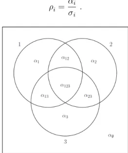
for the fraction who consider only …rms 1 and 2, and so on.) When there are only few …rms the pattern of choice sets can be illustrated using a Venn diagram, and Figure 1 depicts
4The positive analysis which follows is not a¤ected if each consumer has a downward-sloping demand
functionx(p), provided revenuepx(p)is an increasing function up to the monopoly price. However, welfare analysis (for instance in our discussion of entry) requires adjustment with downward-sloping demand.
a market with three …rms.5 Here, a consumer considers a particular subset of …rms if she lies inside the “circle” of each of those …rms. For instance, a fraction 12 of consumers
consider the two …rms 1 and 2.
A consumer is captive to …rm i if she considers i but no other other …rm, and there is a fraction i of such consumers. The reach of …rm i is the set of consumers who consider
the …rm, and the fraction of such consumers is denoted i, so that
i =
X
Sji2S S :
Finally, thecaptive-to-reach ratio of …rm i is denoted i, where
i = i i
:
Figure 1: Choice sets with three …rms
Firms compete in a one-shot Bertrand manner, and a consumer buys from the …rm she considers that has the lowest price (provided this price is no greater than 1). In particular, a …rm o¤ers a uniform price to all its potential customers, and cannot make its price to a consumer contingent on the choice set of that consumer.6 If two or more …rms choose
the same lowest price, we suppose that the consumer is equally likely to buy from any
5In a spatial context this Venn diagram has a more literal interpretation: if consumers only consider
buying from a …rm within a speci…ed distance, then the locations of …rms determine the centre of the circles on the diagram. With more …rms (and a …nite set of consumers), consideration sets can be conveniently depicted using a bipartite graph, where the two groups in the graph are the consumers and the …rms, and a line connecting a consumer to a …rm corresponds to the former considering the latter. In a very di¤erent context, Prat (2018) uses a model of consideration sets similar to that presented here.
6In Armstrong and Vickers (2019) we investigate the impact of …rms being able to o¤er di¤erent deals
such …rm. Since industry pro…t is a continuous function of the vector of prices chosen, Theorem 5 in Dasgupta and Maskin (1986) shows that an equilibrium exists. Since an individual …rm’s pro…t is usually discontinuous in the price vector, the equilibrium will usually involve mixed strategies for some …rms. We make assumptions to rule out some extreme and uninteresting con…gurations. The …rst requires that there be some interaction between …rms:
Assumption 1: Some consumers consider at least two …rms.
(If all customers were captive, each …rm chooses p 1 for sure.) The second assumption prohibits the possibility that a subset of …rms choose the competitive price p 0 for sure, as such …rms play no important role in the analysis:
Assumption 2: Every non-empty subset of …rms S contains at least one …rm with con-sumers within its reach who consider no other …rm inS.
For instance, this assumption rules out the situation where two …rms reach precisely the same set of consumers. Intuitively, Assumption 2 ensures that no subset S of …rms will setp 0, since there is a …rm in S which has some customers with no overlap with other …rms in S, and this …rm can pro…tably raise its price above zero. These two assumptions together imply that there is no equilibrium in pure strategies, and at least some …rms choose their price according to a mixed strategy.
When …rmichooses pricep 1it will sell to a consumer when that consumer is within its reach and when none of the other …rms the consumer considers o¤ers a lower price. Therefore, when rival …rms j 6= i choose price according to the cumulative distribution function (CDF) Fj(p), …rm i’s expected demand with price p 1is
qi(p) X Sji2S S 0 @Y j2S=i (1 Fj(p)) 1 A : (1)
Here, the sum is over all consumer segments which consider …rm i, and for each such segment the product is over all rivals for …rm i in that segment. (If there are no such rivals, i.e., when the segment comprises …rm i’s captive customers, we use the convention that this product equals 1.7) Equilibrium occurs when for each …rmi there exists a pro…t
7Expression (1) is written without taking into account the possibility of ties; however, Lemma 1 shows
level i and a CDF Fi(p) such that …rm i’s pro…t pqi(p) is equal to i for every price in
…rmi’s support and no higher than i for any price outside its support.8
The following result collects a number of observations about the structure of price competition in equilibrium, some of which are familiar from the existing literature.9
Lemma 1 In any equilibrium:
(i) …rm iobtains pro…t i i, with equality for at least one …rm, and the minimum price
in its support is no smaller than i;
(ii) each …rm obtains positive pro…t (even if it has no captive customers) and p0, the
minimum price chosen by any …rm, is positive;
(iii) each …rm’s price distribution is continuous (that is, has no “atoms”) in the half-open interval [p0;1);
(iv) each price in the interval [p0;1] lies in the price support of at least two …rms;
(v) if there are three or more …rms, there is at least one price which lies in the support of three or more …rms, and
(vi) p0 lies weakly between the second lowest i and the highest i. If the …rm with the
highest i has p0 in its support then p0 is equal to the highest i.
Proof. All proofs are contained in the appendix.
Comparative statics with regard to market changes can naturally be studied within this framework of limited choice sets. For instance, entry by a new …rm can be modelled as a new “circle” superimposed onto the existing Venn diagram. That is, entry does not a¤ect which consumers consider the incumbent …rms, and the reach of an incumbent …rm is una¤ected by entry, although its number of captive customers will weakly fall.10
Since welfare (consumer surplus plus industry pro…t) is the total number of consumers reached, it follows that entry (if it is costless) will weakly increase welfare. Likewise, if entry reduces industry pro…t it will bene…t consumers. Mergers also have a natural set-theoretic interpretation in this framework: when two or more …rms merge we assume that the merged entity sets the same price to all its customers, and that the set of consumers
8As usual, the support of …rmi’s price distribution is de…ned to be the smallest closed set P [0;1]
such that the probability that the …rm chooses a price inP equals one.
9For instance, see McAfee (1994, page 28).
10In particular, there is no danger of “choice overload”, whereby the number of consumers who compare
who consider the merged entity is the union of the sets of consumers who considered the separate …rms.11 Thus, a merger (with no accompanying cost synergies) has no impact
on welfare, and harms consumers if and only if it increases industry pro…t. Note that the fraction of consumers reached by the merged …rm is no greater than the sum of those reached by the separate …rms, while the captive base of the merged …rm is no smaller than the sum of captives of the separate …rms. Finally, a market expansion can be modelled as an increase in the fractions of consumers in each non-empty segment of the Venn diagram (taken from the consumer segment ; who previously had no choice).
As discussed in the introduction, previous work has studied the cases with symmetric …rms, with independent reach, and where consumers are either captive to one …rm or can choose from all …rms, and we next describe those cases and add comments about entry and mergers.
Symmetric …rms: Burdett and Judd (1983, section 3.3) study a market with n 2 sym-metric …rms and where consumers consider …rms at random (a speci…ed fraction consider one random …rm, a speci…ed fraction consider two random …rms, and so on). This model can be generalised somewhat so that …rms are symmetric but choice sets need not be ran-dom. Speci…cally, suppose that each …rm has a1 captive customers, a2 consumers who
consider exactly one other …rm (not necessarily random), and in general am consumers
who considerm 1other …rms for m n. Let
(x) a1+a2x+a3x2+:::+anxn 1
be the probability generating function associated with the number of rivals faced by a …rm. Here, (x)is convex and increasing, the number of captive customers for each …rm is (0), each …rm has reach = (1) and captive-to-reach ratio = (0)= (1). Assumptions 1 and 2 imply 0< (0)< (1).
In a symmetric market, the unique symmetric equilibrium (which is not necessarily the only equilibrium) is derived as follows. Each …rm obtains equilibrium pro…t i (0) and
has the minimum price . When each of its rivals uses the CDFF(p), a …rm’s demand with price p 1 in (1) is q(p) = (1 F(p)). Since each …rm makes pro…t (0), the symmetric
11An alternative approach would be for the merged entity to maintain separate brands and to be able
equilibrium CDF satis…es
(1 F(p)) (0)
p ; (2)
and the function F(p)strictly increases from 0 to 1 as p increases from to 1.
The models in Rosenthal (1980) and Varian (1980) are special cases of this framework, where consumers either consider one random …rm or consider all …rms, so thatam = 0 for
1< m < n. With this pattern of consideration, Baye et al. (1992) show that when n 3
there are multiple equilibria (all of which involve the same pro…t for …rms). For instance, one asymmetric equilibrium has all but two …rms choosing p = 1 for sure, selling only to their captive customers, while the remaining two …rms choose prices on the interval [ ;1]. In general, entry by a new …rm into a symmetric market has ambiguous e¤ects on industry pro…t and consumer surplus, as we discuss in more detail in section 4. However, a merger between two or more …rms in a symmetric market is always pro…table. Before merger each …rm obtained pro…t equal to its captive base, and a merger can only increase the merged entity’s number of captive customers. A merger cannot decrease the pro…t of the non-merging …rms (since they still obtain at least their captive pro…t), and so the merger increases industry pro…t and harms consumers. Finally, in this symmetric con…guration there are “search externalities”, in the sense that an increase in the number of consumers who consider more than one …rm (i.e., an increase in am for some m 2) will bene…t all existing consumers (including those captive to a …rm). To see this, note that an increase inam for m 2induces a rise in the F(p) which solves (2), and so each …rm will lower its price in the sense of …rst-order stochastic dominance.
Independent reach: Ireland (1993) and McAfee (1994) study the situation where each …rm has an independent chance of being considered by a consumer. Speci…cally, …rm i
is considered by an independent fraction i of the consumer population, where …rms are
labelled so that 0 < 1 2 ::: n 1. (Assumption 2 requires n 1 < 1.) The
fraction of consumers captive to …rmi is i = i j6=i(1 j) and so this …rm’s
captive-to-reach ratio is i = j6=i(1 j). Thus the …rm with the largest reach is also the …rm with
the highest captive-to-reach ratio n= ni=11(1 i).
Firm i sells to a consumer when it chooses price p if it reaches that consumer (which occurs with probability i) and no rival reaches that consumer with a lower price. If …rm j chooses its price with the CDF Fj(p), the probability that …rm j reaches the consumer
with a lower price is jFj(p). Therefore, …rm i’s demand with pricep 1 in (1) takes the multiplicatively separable form
qi(p) = i
Y
j6=i
(1 jFj(p)) : (3)
Ireland (1993) and McAfee (1994) show that the equilibrium is such that all …rms have the same minimum pricep0 = n, and the pro…t of …rm iis i = ip0. Thus, …rms’ pro…ts
are proportional to their reaches, and the pro…t of the largest …rm is equal to its number of captive consumers, while the pro…t of smaller …rms is weakly greater than their number of captive consumers. The CDFs which support these equilibrium pro…ts are such that …rm i chooses its price with interval support [p0; pi], where …rm i’s maximum price pi is
smaller for smaller …rms. The two largest …rms choose prices with support [p0;1], so that
the maximum prices satisfy p1 p2 ::: pn 1 =pn= 1.
Industry pro…t is = (Pni=1 i)p0, total welfare is the fraction of consumers who
consider at least one …rm which is 1 (1 n)p0, and the di¤erence between welfare and
pro…t is consumer surplus
CS= 1 1 +
nP1
i=1
i p0 : (4)
Consumer surplus does not depend on the reach of the largest …rm, n, but increases with
the reach of each smaller …rm.
The model with independent reach has intuitive properties with respect to entry and mergers. Entry by a …rm which also has independent reach will increase consumer surplus (4). If the entrant is not the largest …rm in the market, so its reach is E < n, then the
minimum price p0 falls by the multiplicative factor (1 E) which outweighs the impact
of the additional E in the sum in the term ( ) in (4).12 If two …rms i and j merge, the
merged entity has independent reach i + j i j. Since this combined reach is lower
than the sum of the pre-merger reaches, the only way the merger can be pro…table is if the minimum pricep0 rises after the merger, in which case the non-merging …rms also increase
their pro…t after the merger.13 A pro…table merger must therefore increase industry pro…t,
and so reduce consumer surplus.
12If the entrant is the largest …rm in the market, then the same analysis applies with
n replacing E.
13It is only possible for a merger to raise the minimum price if the merged entity is the largest …rm in
the post-merger market. For instance, one can check that a merger between the two largest …rms is always pro…table.
One-or-all choice: Suppose there are n 2 …rms, where > 0 consumers consider all …rms and i consumers consider only …rm i. No consumers consider intermediate numbers
of …rms, and so the reach of …rmiis i = + i. We have already discussed the symmetric
case 1 =:::= n, so as in Baye et al. (1992, Section V) suppose that 1 < 2 < ::: < n.
Suppose …rst that n= 2, which is the situation studied by Narasimhan (1988). Lemma 1 then determines the unique equilibrium, which is that both …rms have the same support for prices, [p0;1], where p0 = 2= 2 is the larger captive-to-reach ratio, and …rm i = 1;2 has
pro…t i = ip0. To maintain indi¤erence for …rmj, the CDF used by …rmiin equilibrium,
Fi, satis…es
p[ j Fi(p)] jp0 : (5)
Similarly to independent reach, the smaller …rm’s pro…t exceeds its captive pro…t 1 while
the larger …rm obtains exactly its captive pro…t. Industry pro…t in equilibrium is
= ( 1+ 2)p0 = 1+ 2 1
2
: (6)
One can check that industry pro…t increases with each portion in the Venn diagram (i.e., with 1, 2 and ), so that any market expansion boosts industry pro…t. Total welfare is
the total number of consumers reached,W = 1+ 2 , and consumer surplus is therefore
CS = 1
2
:
Thus, keeping reaches constant, consumer surplus increases when the overlap is larger, even though fewer consumers are then served. Likewise, consumer surplus decreases when the larger …rm’s set of captive customers expands, keeping the other regions of the Venn diagram unchanged, even though more consumers are served.
To extend this analysis to more than two …rms, introduce additional …rms i= 3; :::; n, all with i > 2. If the smallest …rms, 1 and 2, continue to use the price strategies (5), one
can check that each …rmi 3is better o¤ choosing the monopoly pricep= 1than to o¤er any lower price. Thus it is an equilibrium for the two smallest …rms to follow the above duopoly strategies, and for all larger …rms to serve only their captive base and choose the monopoly price for sure.14 The result is that all …rms except the smallest one obtain their
captive pro…t, and only the two smallest …rms ever choose prices below the monopoly level.
In this framework a merger between …rms, falling short of a merger to monopoly, leaves the number of captive customers unchanged. As a result, almost all pair-wise mergers leave the merged entity’s pro…t unchanged or cause it to fall. In fact, in contrast to independent reach, the only way a pair of …rms could pro…tably merge is if the merged …rm is the smallest …rm in the post-merger market. Such a merger has no impact on the non-merging …rms’ pro…ts and so increases industry pro…t and harms consumers.
In the remainder of the paper we show that other, richer possibilities exist outside these special cases. We start in the next section by describing how a radically di¤erent kind of equilibrium can arise when …rms have nested reach.
3
Nested reach
The situation with independent reach has all consumers being equally likely to be reached by a …rm, regardless of which other …rms they consider. At the other extreme one could envisage consideration sets as being nested, in the sense that if …rm i reaches a greater fraction of consumers than …rmj, all …rmj’s consumers also consider …rmi. For example, an entrant’s reach lies inside an incumbent’s reach if only a subset of latter’s existing customers are willing to consider buying from the entrant. Likewise, if consumers consider options in an ordered fashion, as may be the case with internet search results (where some consumers just consider the …rst result, others consider the …rst two, and so on), then the reach of a lower ranked option is nested inside that of a higher ranked option. Alternatively, if consumers only consider the …rms whose product they …nd suits their tastes, then low-quality …rms might be considered by only a subset of the consumers who consider a higher-quality …rm. With nested reach, only the largest …rm has any captive customers, and a smaller …rm has positive demand only if its price is below all the prices of larger …rms.
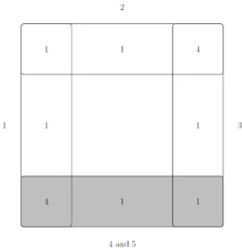
As depicted in Figure 2, suppose there are n 3 …rms with nested reach. Let …rm i
have reach i, where …rms are ordered as 0 < 1 < 2 < ::: < n, and for i 2 write i = i i 1 for the incremental reach of …rm i. While it is hard to …nd the equilibrium
in all nested situations, the following result describes equilibrium in those cases where incremental reach is larger for larger …rms.
Proposition 1 Suppose n 3 …rms have nested reach such that
0< 2 ::: n : (7)
Then there is an equilibrium with price thresholds p1 < p2 < ::: < pn 1 < pn= 1 such that
the price support of …rm 1 is [p1; p2], the support of …rm n is [pn 1; pn], and the support of
…rm 1< i < n is [pi 1; pi+1]. Thus, only …rms i and i+ 1 (where 1 i < n) choose prices
in the interval (pi; pi+1). The thresholds are determined recursively by p2 = 1+ 2
2 p1 and
for 1< i < n
pi+1 =pi+ i
i+1
pi 1 ; (8)
where p1 is chosen to makepn= 1. The pro…t of …rm 1 is 1 = 1p1 and the pro…t of …rm
i >1 is i = ipi.
The format of this equilibrium consists of “overlapping duopolies”, where each price is in the support of exactly two …rms,15 and where smaller …rms only choose low prices while
larger …rms only choose high prices.16 In this sense there is segmented price competition
rather than head-to-head price competition, even though there is head-to-head competition in terms of consumer consideration (as …rm 1’s potential customers consider all …rms). Nevertheless, the presence of large …rms a¤ects the pro…ts of smaller …rms, and (except for the very largest …rm)vice versa.
To illustrate, consider the case where reach decays with a constant rate of attrition, so that the reach of …rmi= 1; :::; nis i = n i. In this case i = n i(1 )which increases
with i as required for Proposition 1, and equation (8) becomes pi+1 = pi+ pi 1. When
n= 2 the two …rms have reaches 1 = 1 and 2 = 1, and the duopoly analysis in section
2 shows that the minimum price is1 and industry pro…t is 2 = 1 2. When n= 3,
Proposition 1 implies that the two threshold prices arep1 = 1+ (11 ) andp2 = 1+ (11 ) and
that industry pro…t is 3 = 1
2
1+ (1 ). Both 2 and 3 decrease from 1 to 0 as increases
from 0 to 1. Perhaps surprisingly, though, when 0 < < 1 the pro…t with three …rms is
15With the exception of the threshold pricesp
2; :::; pn 1, which are in the support of three …rms.
16A similar pattern of segmented pricing is seen in Bulow and Levin (2006). They study a matching
model where n heterogeneous …rms each wish to hire a single worker from a pool with n heterogeneous workers, where the payo¤ from a match is (in the simplest version of their model) the product of qualities of the …rm and worker. Firms choose wages which they must pay regardless of the quality of the worker eventually hired, workers care only about their wage, and higher quality workers choose their employer …rst. In equilibrium, …rms o¤er wages according to mixed strategies, where higher quality …rms o¤er wages in a higher range than lower quality …rms.
strictly higher than with two …rms. Since the change from n = 2to n = 3corresponds to entry by a third …rm with reach 2 into the duopoly market, this implies that entry of this formraises industry pro…t.17 Since no new consumers are served by the entrant, it follows
that entry harms consumers in aggregate, even though the minimum price o¤ered in the market is lower after entry.
Figure 2: Three …rms with nested reach
Proposition 1 can be used to obtain an expression for industry pro…t with any n. However, the analysis simpli…es in the limit with many …rms, when one can show that the threshold prices are given by the geometric progression ; 2; :::, where = 2
1+p1+4 1,
and the minimum price o¤ered converges to zero. Industry pro…t is 1 = (1 )(1 + + ( )2+:::) = 1
1 . This limit pro…t also decreases from 1 to 0 as increases, and
satis…es 2 < 1 < 3 when 0 < < 1. Thus entry has a non-monotonic e¤ect on
industry pro…t, …rst increasing and then decreasing pro…t (although the limit pro…t with many …rms remains above that with duopoly). We discuss the possibility that entry can harm consumers in more detail in the next section, using a more transparent framework with symmetric incumbents.18
Proposition 1 describes equilibrium only for cases where incremental reach weakly in-creases. In the next section we thoroughly analyse our general framework in the case of triopoly, and …nd that overlapping duopoly pricing is by no means special to the nested con…guration. We will also obtain results that imply for the case of nested reach that
17Entry does not a¤ect the pro…t of the largest …rm, which obtains its captive pro…t in either case, but
it reduces the pro…t of the smaller incumbent. However, the pro…t obtained by the entrant outweighs the lost pro…t of this incumbent.
18Another case which is easily solved is when incremental reach
iis constant, in which case (8) entails
(i) when 3 > 2 the equilibrium in Proposition 1 is unique and (ii) when 3 < 2 the
equilibrium instead has all three …rms using the same minimum price. However, in the latter case we will see that the largest …rm can sometimes have a gap in its price support, so that it charges high and low prices but not intermediate prices.
4
The three-…rm problem
In all the asymmetric con…gurations considered so far (independent reach, “one-or-all” choice, and nested reach) there is a clear-cut ordering of the …rms, in the sense that a …rm with a larger reach also has a weakly higher captive-to-reach ratio. More generally, though, these two ways to order …rms need not coincide. For instance, a “niche” …rm could have limited reach but have a high proportion of its reach being captive. In this section we allow for general patterns of consumer consideration in the context of triopoly.
Consider the triopoly market shown on Figure 1. For each pair of …rms i and j de…ne
ij = ij +
i j ;
where to simplify notation we have written = 123. The parameter ij re‡ectscorrelation
in the reach of …rms i and j: i and j are the respective probabilities that a consumer
considers …rmi and …rm j while ( ij + ) is the probability she considers both …rms, and
so ij is above or below 1 according to whether consideration of …rm i is positively or negatively correlated with consideration of …rm j. With independent reach we have all
ij = 1, while if the reach of …rms i and j is disjoint then ij = 0. The pair of …rms with
the largest ij can be thought of having the “strongest interaction” in the market. As we will see, if only two …rms choose the lowest price p0 in equilibrium, while the third …rm
only uses higher prices, they will be the pair of …rms with the largest ij. Similarly, write
=
1 2 3
;
which is again equal to 1 with independent reach. Note that k ij for distinct i, j
and k, with equality if and only if ij = 0. For simplicity, if Fi(p) is …rm i’s CDF for
price in equilibrium writeGi(p) iFi(p), so thatGi increases from zero to i. Using this
notation, …rmi’s demand at pricep in (1) is
= i+ FjFk ( + ij)Fj ( + ik)Fk (9)
= i[1 + GjGk ijGj ikGk]: (10)
Our main result in this section shows that the form of equilibrium depends on whether or not the interactions between …rms, measured by ij, are similar or asymmetric.
Proposition 2 Suppose that …rms are labelled so that …rms 2 and 3 have the strongest interaction, i.e., 23 maxf 12; 13g.
(i) If
minf 2; 3g< 12+ 13 23 (11)
then in equilibrium all …rms have the same minimum pricep0, which is the highest
captive-to-reach ratio among the …rms; (ii) If
minf 2; 3g> 12+ 13 23 (12)
then equilibrium takes the form of “overlapping duopoly”: if …rms 2 and 3 are labelled so
3 2, then there are prices p0 and p1, with p0 < p1 1, such that …rm 3 has price
support [p0; p1], …rm 2 has support [p0;1] and …rm 1 has support [p1;1]. (If 2 = 3 then
p1 = 1 and …rm 1 chooses p 1 for sure.) Explicit expressions for the thresholds p0 and
p1, as well as for the pro…ts of the three …rms, are given in the proof.
This result shows that only limited kinds of pricing patterns can emerge in equilibrium. For example, it cannot be that two …rms choose prices over a range [p0;1]while the third
…rm only chooses from an intermediate or upper range of prices.
Part (i) of this result applies when interactions are similar across pairs of …rms (and where some consumers consider exactly two …rms so that k < ij), as is the case with
independent reach. Indeed, part (i) applies if the two pairs with the greatest interaction have a similar interaction: if say 23 = 13 12 and there are some consumers who
consider exactly two …rms then condition (11) is satis…ed. In particular, if in the statement of Proposition 2 there is a “tie” for which pair of …rms has the strongest interaction, then part (i) must apply. With nested reach the two smallest …rms have the strongest interaction and condition (11) requires that incremental reach is smaller for larger …rms. Thus with three nested …rms, the cases not covered by Proposition 1 have all …rms using the same minimum price.
Part (ii) applies when one pair of …rms has signi…cantly stronger interaction than other pairs. For instance, if …rms 2 and 3 are considered by almost the same set of consumers (so their circles on the Venn diagram almost coincide), and if 1 > 0, then …rms 2 and
3 have the greatest interaction and condition (12) is satis…ed, and …rm 1 chooses price
p 1. Intuitively, when two …rms reach nearly the same set of consumers, they compete …ercely between themselves, leaving the remaining …rm to price at or near the monopoly level. Likewise, if …rm 1 has a large captive base so that 1 is large (and when …rms 2 and
3 have some overlap), then …rms 2 and 3 have the greatest interaction and condition (12) is satis…ed. With nested reach, condition (12) requires that incremental reach is larger for larger …rms, thus verifying Proposition 1. Another situation where (12) holds is the “one-or-all” speci…cation in Baye et al. (1992, Section V), where no consumer considers exactly two …rms and 1 > 2 3, in which case ij = =( i j)and the two smallest …rms 2 and
3 have the greatest interaction. Yet another con…guration where part (ii) applies is when two …rms have disjoint reach, so that 13 = = 0 say, in which case (12) holds whenever
12 6= 23. Thus the only way that two …rms can have overlapping price supports is if they
have overlapping reach.
In the knife-edge case where
minf 2; 3g= 12+ 13 23 ; (13)
which is not covered by Proposition 2, there is the possibility that both kinds of equilibrium coexist. For instance, this is so in the symmetric Varian-type market where 12 = 13 = 23 = 0 and 1 = 2 = 3, where there is a symmetric equilibrium where all …rms price
low and also asymmetric equilibria where one of the …rms choosesp 1. (See Baye et al. (1992) for the full range of equilibria in this market.)
Equilibrium strategies when all …rms use the same minimum price: Proposition 2 provided much information about equilibria in this model—it characterises equilibrium pro…t and consumer surplus in the two regimes, and it describes equilibrium strategies when part (ii) applies. However, it does not describe equilibrium pricing strategies for part (i), and the equilibrium patterns of prices turn out to have interesting economic properties.
In the earlier version of this paper (Armstrong and Vickers, 2018, Proposition 2) we calculated an equilibrium whenever part (i) applied (without showing if it was unique), and this took one of two forms: either (a) the three …rms were active in a lower price range
and then two were active in a range of higher prices, or (b) the three …rms were active in a lower price range, then only the most competitive pair were active in an intermediate price range, and then another pair of …rms were active in a higher range. In particular, in situation (b) one …rm (…rm 1 using the labelling in Proposition 2) chose low and high prices, but not intermediate prices.
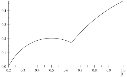
0.2 0.3 0.4 0.5 0.6 0.7 0.8 0.9 1.0 0.0 0.1 0.2 0.3 0.4 p
Figure 3: “Ironing” in a nested market with 1 = 1=2, 2 = 4=5, 3 = 1
The general analysis was complicated, and here we merely report an example to show the possibility. Suppose three …rms have nested reach, where 3 = 12, 2 = 45 and 1 = 1.
We show in the appendix that equilibrium with this pattern of choice sets has all …rms choosing prices in the range [1
5; 9
25], …rms 2 and 3 choosing prices in the range [ 9 25;
16 25] and
…rms 1 and 2 choosing prices in the range[16
25;1]. The reason why the largest …rm has
non-convex price support can be explained as follows. When all …rms price low in equilibrium, so that part (i) of Proposition 2 applies, one can calculate that the three CDFs increase inpfor prices just above p0, the minimum price. (This is ensured by condition (11).) One
can also calculate the smallest price,p1 say, at which some CDF reaches 1 and above which
the two remaining …rms compete as duopolists for prices up to 1. (In the nested case, it is the smallest …rm’s CDF which …rst reaches 1, although in the general model more detailed analysis is required to determine which …rm …rst drops out.)
However, in some cases—as in this example—…rm 1’s candidate CDF (i.e., when we ignore the monotonicity constraint on the CDF) starts to decrease inp before the largest CDF reaches 1, which cannot therefore be a valid CDF. Figure 3 illustrates …rm 1’s can-didate CDF if we ignored its monotonicity constraint. The correct CDF for this …rm is
then obtained by “ironing” this curve as shown on the …gure, so that the largest …rm does not choose prices in the interval denoted by the dashed line, which in this example is the interval (9
25; 16
25). (This CDF does not reach 1 since this …rm has an atom at p = 1 in
equilibrium.)
The equilibria with ironing—when one …rm’s price support has a gap in the middle— provide insight into the relationship between the two seemingly contrasting parts of Propo-sition 2. A con…guration which is “well inside” the parameter space de…ned by (11) will have a pattern of prices similar to that with independent reach: all three …rms choose low prices, then …rm 3 drops out leaving …rms 1 and 2 to compete in the range with high prices. As parameters change to approach the boundary (13), the candidate CDF for …rm 1 will start to decrease before …rm 3’s CDF reaches 1. In this case, the “ironing” proce-dure is used so that …rm 1’s price support has a gap in the middle. As the boundary (13) is reached, the lower price range where all three …rms are active shrinks and ultimately vanishes, leaving an equilibrium of the overlapping duopoly form when parameters lie in the region (12).
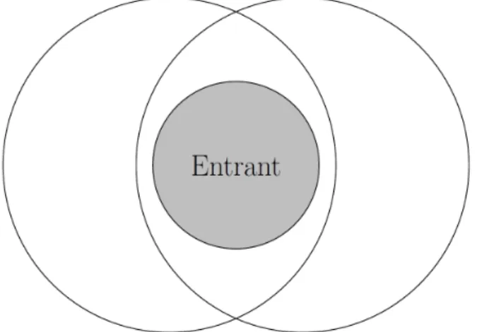
The impact of entry: As an application of this analysis, consider the impact of entry by a third …rm into a duopoly market. If the three …rms have independent reach, then as discussed in section 2 entry will always increase consumer surplus. Beyond this case, however, the analysis is less clear cut. Entry might induce an incumbent to retreat towards its captive base by raising its price, thereby harming its captive customers. This is the case, for example, when the set of consumers reached by the entrant approximately coincides with the set reached by one of the incumbents. Then these …rms will set prices p 0, while the other incumbent chooses p 1 and almost fully exploits its captive customers. Nevertheless, since entry of this form reduces industry pro…t, consumers overall will bene…t. In section 3 we have already seen examples where entry harms consumers overall. These involved nested reach with a constant rate of decay in consideration, where entry by a third smaller …rm induced overlapping duopoly pricing with the result that the minimum price fell after entry. This kind of nested entry does not a¤ect the number of captive customers in the market. More generally, when entry only occurs within contested segments there is a tendency for entry to harm consumers overall.
by those consumers who already consider both incumbents, as shown on Figure 4. This pattern of consideration is reasonable if only “savvy” consumers consider buying from the entrant, and these are the consumers who are already able to consider both incumbents. In this case part (i) of Proposition 2 applies to the post-entry market (provided the entrant’s reach lies strictly inside the incumbents’ overlap). The minimum price is equal to an incumbent’s captive-to-reach ratio, which is unchanged with entry. Thus, entry of this form leaves welfare and incumbent pro…t una¤ected, increases industry pro…t due to the pro…t obtained by the entrant, and so harms consumers. In fact, it is perfectly possible that even the consumers who consider all three …rms are harmed by this form of entry, despite being able to choose among more …rms, as the higher prices o¤ered by incumbents leave the entrant relatively free to set high prices too.
Figure 4: Entry into the contested market
This result is related to Rosenthal (1980), where entry by a new …rm causes the average price paid by both captive and informed consumers to rise. However, in his model the entrant arrives with its own new pool of captive customers, thus raising welfare, whereas the e¤ect arises in our scenario despite the entrant having none.19
The impact of market expansion: Another informative comparative statics exercise is to consider the impact of a market expansion. An old intuition is that an increase in the
num-19Relatedly, in a setting with di¤erentiated products, Chen and Riordan (2008) show how entry to a
monopoly market can induce the incumbent to raise its price. For instance, entry by generic pharmaceuti-cals might cause a branded incumbent to raise its price, as it prefers to focus on those “captive customers” who care particularly about its brand. Closer to the consideration set framework is Chen and Riordan (2007), who study a model with symmetric …rms, where consumers either consider a single random …rm or consider a random pair of …rms. Among other results, they show that the equilibrium price can increase when an additional …rm enters.
ber of comparison shoppers—consumers who compare prices from several …rms—induce …rms to lower their prices, which bene…ts all consumers including captives. As discussed in section 2, this is true in a symmetric market where an increase in the number of consumers who considerm 2…rms induces all …rms to reduce their prices. However, this is less clear more generally. If the interaction between one pair of …rm increases disproportionately, this could give a third …rm an incentive toraise its price, thereby harming its captive cus-tomers. To illustrate, starting from a symmetric triopoly market, if we increase 23 then
part (ii) of Proposition 2 will eventually apply, in which case …rm 1 will focus on exploiting its captive base and choosep 1. Thus, increased interaction between two …rms can harm the captives of a third …rm.20
Consider next the impact of a market expansion on industry pro…t. With duopoly, we have seen that an increase in any or all of the three parameters 1, 2and 12must increase
industry pro…t (although it might reduce one …rm’s pro…t). With duopoly, increasing the size of the overlap region 12will intensify competition (in the sense that the minimum price
p0is reduced), but this is outweighed by impact on each …rm’s reach so that( 1+ 2)p0rises.
With triopoly, by contrast, increasing the fractions in some regions of the Venn diagram can intensify competition to an extent that outweighs the market expansion e¤ect, so that industry pro…t falls. To see this, consider a triopoly market where part (i) of Proposition 2 applies, in which case industry pro…t is
= ( 1+ 2+ 3)p0 ; (14)
where p0 is the highest captive-to-reach ratio. If …rm 1 has the highest captive-to-reach
ratio, then a small increase in that …rm’s overlap regions 12, 13 or will keep the form of
the equilibrium unchanged, but the minimum pricep0 will fall. Firm1’s pro…t is unchanged
(since it obtains its captive pro…t regardless), and one can calculate that the impact on industry pro…t (14) of an increase in 12or 13is negative if 1 < 2+ 3, while an increase
in reduces pro…t if2 1 < 2+ 3.
20A similar e¤ect can occur when the fraction of consumers who consider all three …rms rises. For
instance, suppose consumer segments are (proportional to) 1= 3and 2 = 3= 12 = 13= 23 = 1,
then for any …rms 2 and 3 are the most competitive pair, and for small part (i) of the proposition applies, while if is increased part (ii) eventually applies in which case …rm 1 chooses p 1. Here, an increase in a¤ects the interaction between …rms 2 and 3 disproportionately, and pushes the market towards segmented pricing.
The impact of a merger: We discussed in section 2, within the three special patterns of consideration described there, how a pro…table merger harmed consumers overall. We now show that the same is always true in the three-…rm case. Speci…cally, we show that a pro…table merger between two …rms necessarily increases the third …rm’s pro…t. Suppose that …rmN is the one not merging. IfN’s pre-merger pro…t was equal to its captive pro…t
N, the merger of the other two …rms clearly cannot reduce that. If N’s pre-merger pro…t
was equal to Np0—i.e., its reach times the minimum price—then the merger between the
other two will increase N’s pro…t because the minimum price must rise for the merger to be pro…table.21 The only remaining possibility is a merger between …rms 2 and 3 in the
conditions of part (ii) of Proposition 2 where, moreover, …rm 2 has an atom atp= 1. We show in the appendix that a pro…table merger increases1’s pro…t in this case too. Therefore pro…table mergers in the three-…rm case never reduce the pro…t of the non-merging …rm, in which case industry pro…t rises. We deduce that any pro…table merger is detrimental to consumers.
Figure 5: A pro…table merger which bene…ts consumers
However, it is not true in general, with more than three …rms, that pro…table mergers harm consumers. It may be, for example, that a merger between two …rms with a strong interaction—which is therefore likely to be pro…table—might induce non-merging …rms to “enter the fray” and compete for the newly-pro…table consumer segment, with the result that overall industry pro…ts might fall and consumers are made better o¤. To illustrate
21Before the merger, the combined pro…t of the merging …rms, say …rmsA and B, was at least(
A+ B)p0, and since their combined reach falls after the merger, for the merger to be pro…table the minimum
this possibility consider the following example, which draws from our analysis of triopoly together with the symmetric case from section 2. Figure 5 shows the pattern of consumer consideration. There are initially …ve …rms, where …rms 4 and 5 reach precisely the same set of consumers (depicted as the shaded set) and hence set price p = 0 in equilibrium. Firms 1, 2 and 3 each have a single captive customer, a single consumer considers each set of …rmsf1;2gand f3;4;5g, while four consumers consider each set of …rms f2;3g and
f1;4;5g. (No consumers consider more than three …rms.)
Since …rms 4 and 5 set price zero, …rms 1, 2 and 3 compete as triopolists as if the shaded row on Figure 5 was eliminated. Here, …rms 2 and 3 have the greatest competitive interaction in this triopoly, and Proposition 1 implies that equilibrium takes the overlapping duopoly form with …rms 2 and 3 setting low prices and …rms 1 and 2 setting high prices. The proof of part (ii) of the Proposition shows that …rm 1 obtains its captive pro…t ( 1 = 1),
while …rms 2 and 3 obtain respective pro…ts 2 = 6p0 and 3 = 5p0, where p0 = 27 is the
minimum price. Since …rms 4 and 5 make zero pro…t industry pro…t is 297 . Due to the asymmetry between …rms, industry pro…t substantially exceeds the captive pro…t, 3.
Now suppose …rms 4 and 5 merge. (Clearly this is a pro…table merger, as before the …rms obtained no pro…t.) The symmetry of the market implies that each …rm now obtains its captive pro…t ( i = 1), so that industry pro…t falls to 4 after the merger, and consumers
overall are better o¤. Intuitively, before the merger the market was highly asymmetric, which allowed …rms to enjoy high pro…ts, and the merger brings more intense symmetric competition to the market. This example shows that not all pro…table mergers in our setting are detrimental to consumers, but such competition-enhancing mergers appear to be relatively rare.
5
Conclusions
The aim of this paper has been to explore, in a parsimonious framework with price-setting …rms and homogeneous products, how the structure of consumer choice sets matters for the nature of equilibrium price dispersion. The analysis has yielded a number of results that we did not initially expect.
First, we found equilibria with segmented pricing patterns, i.e., with some …rms only pricing high and others only pricing low. Second, in the three-…rm case we established generically either that all …rms set the same minimum price (in which case their pro…t
was proportional to reach), or that pricing was segmented (so that one …rm only set low prices and one set only high prices). In prior literature multiplicity of equilibria has gained considerable attention, and all such cases lie on the knife edge between these two regimes. Third, the key to determining which of the two regimes applies was found to be the proximity or otherwise of the correlation measures of pairwise interaction, and when one pair of …rms had signi…cantly stronger interaction than other pairs then segmented pricing ensued. Fourth, for some parameter con…gurations we found equilibria with a gap in one …rm’s price support, so that that …rm sometimes prices high, and sometimes low, but never in between. Fifth, we found plausible patterns of consumer consideration in which entry is detrimental to consumers because it softens competition between incumbents, leading them to retreat towards their captive base. Likewise, there were situations where an increase in the number of consumers who consider one pair of …rms causes a third …rm to retreat towards its captive base, showing that search externalities need not bene…t all consumers. Sixth, pro…table mergers were shown always to be detrimental to consumers in the three-…rm case, as in the special cases discussed in section 2, but not more generally.
The analysis could be extended in a number of directions. One would be to settings beyond nested reach and the three-…rm case that we have analysed in detail. For example, one could seek more general conditions for equilibrium to take the overlapping duopoly form, or one could try to establish that all …rms use the same minimum price when (ap-propriately generalised) competitive interactions are similar enough. Second, one could investigate policy interventions in these kinds of markets. For example, when would the imposition of a price cap on a large …rm induce other …rms to lower or raise their prices? A third extension would be to endogenise the pattern of choice sets, beyond our analysis of entry and mergers, by introducing search by consumers, word-of-mouth communication between consumers, or advertising by …rms.22 For instance, one could study a model of
non-sequential search where a consumer can determine her choice set S by incurring a speci…ed up-front search cost (increasing in S). Such a framework would generalize Bur-dett and Judd (1983, section 3.2) to allow …rms to be asymmetric and for consumers to target speci…c …rms for consideration. Alternatively, word-of-mouth communication could mean that a …rm’s reach was in‡uenced by the price it o¤ers.
22For instance, in the context of advertising, Ireland (1993) and McAfee (1994) study a sequential model
where …rms …rst invest in reach and then compete in price, while Butters (1977) studies the situation where …rms choose their reach and price simultaneously. (In each case reach is assumed to be independent.)
References
Armstrong, M., and J. Vickers (2018): “Patterns of Competition with Captive Cus-tomers,” Department of Economics Working Paper No. 864, University of Oxford.
(2019): “Discriminating Against Captive Customers,” American Economic Re-view: Insights, 1(3), 257–272.
Banerjee, B., and D. Kovenock(1999): “Localized and Non-localized Competition in the Presence of Consumer Lock-in,” inAdvances in Applied Microeconomics, Vol. 8, ed. by M. Baye, pp. 45–70. JAI Press: Greenwich, CT.
Baye, M., D. Kovenock,and C. De Vries(1992): “It Takes Two to Tango: Equilibria in a Model of Sales,”Games and Economic Behavior, 4, 493–510.
Baye, M., and J. Morgan (2001): “Information Gatekeepers on the Internet and the Competitiveness of Homogeneous Product Markets,”American Economic Review, 91(3), 454–474.
Bulow, J., and J. Levin (2006): “Matching and Price Competition,” American Eco-nomic Review, 96(3), 652–668.
Burdett, K., and K. Judd (1983): “Equilibrium Price Dispersion,” Econometrica, 51(4), 955–969.
Butters, G.(1977): “Equilibrium Distributions of Sales and Advertising Prices,”Review of Economic Studies, 44(3), 465–491.
Chen, Y.,and M. Riordan (2007): “Price and Variety in the Spokes Model,”Economic Journal, 117, 897–921.
(2008): “Price-Increasing Competition,”Rand Journal of Economics, 39(4), 1042– 1058.
Chioveanu, I., and J. Zhou (2013): “Price Competition with Consumer Confusion,” Management Science, 59(11), 2450–2469.
Dasgupta, P., and E. Maskin (1986): “The Existence of Equilibrium in Discontinuous Economic Games, I: Theory,” Review of Economic Studies, 53(1), 1–26.
Draganska, M., and D. Klapper (2011): “Choice Set Heterogeneity and the Role of Advertising: An Analysis with Micro and Macro Data,”Journal of Marketing Research, 48(4), 653–669.
Honka, E., A. Hortacsu, and M. A. Vitorino (2017): “Advertising, Consumer Awareness, and Choice: Evidence From the U.S. Banking Industry,” Rand Journal of Economics, 48(3), 611–646.
Ireland, N.(1993): “The Provision of Information in a Bertrand Oligopoly,” Journal of Industrial Economics, 41(1), 61–76.
Janssen, M., and E. Rasmusen (2002): “Bertrand Competition Under Uncertainty,” Journal of Industrial Economics, 50(1), 11–21.
Johnen, J., and D. Ronayne (2019): “The Only Dance in Town: Unique Equilibrium in a Generalised Model of Price Competition,” mimeo.
Manzini, P., and M. Mariotti (2014): “Stochastic Choice and Consideration Sets,” Econometrica, 82(3), 1153–1176.
McAfee, R. P.(1994): “Endogneous Availability, Cartels, and Merger in an Equilibirium Price Dispersion,” Journal of Economic Theory, 62, 24–47.
Narasimhan, C.(1988): “Competitive Promotional Strategies,”Journal of Business, 61, 427–449.
Piccione, M., and R. Spiegler (2012): “Price Competition Under Limited Compara-bility,” Quarterly Journal of Economics, 127(1), 97–135.
Prat, A. (2018): “Media Power,”Journal of Political Economy, 126(4), 1747–1782.
Rosenthal, R. (1980): “A Model in which an Increase in the Number of Sellers Leads to a Higher Price,”Econometrica, 48(6), 1575–1579.
Smith, H. (2004): “Supermarket Choice and Supermarket Competition in Market Equi-librium,” Review of Economic Studies, 71(1), 235–263.
Sovinsky Goeree, M. (2008): “Limited Information and Advertising in the U.S. Per-sonal Computer Industry,”Econometrica, 76(5), 1017–1074.
Spiegler, R. (2006): “The Market for Quacks,” Review of Economic Studies, 73(4), 1113–1131.
(2011): Bounded Rationality and Industrial Organization. Oxford University Press, Oxford, UK.
Szech, N.(2011): “Welfare in Markets where Consumers Rely on Word of Mouth,” mimeo.
Varian, H.(1980): “A Model of Sales,” American Economic Review, 70(4), 651–659.
Technical Appendix
Sketch proof of Lemma 1: We …rst discuss arguments to do with deletion of dominated prices. In any equilibrium we have i i, since …rm i can ensure at least this pro…t by
choosing price equal to 1 and serving its captive customers. For this reason, no …rm would ever o¤er a price below i, its captive-to-reach ratio, since if it did so it would obtain pro…t below i even if it supplied its entire reach.
To see that every …rm makes positive pro…t we invoke Assumption 2. There is at least one …rmiwhich has captive customers, and which will not set price below i >0. (Clearly
this …rm makes positive pro…t.) From the remaining …rms, at least one …rm j has captive customers in the subset of …rms excluding i, and so this …rm can set price i and be sure
to obtain positive pro…t. Firm j therefore also has a positive lower bound on its prices. Following the same argument, a …rm in the subset of …rms excluding both i and j can obtain positive pro…t, and so on until the set of …rms is exhausted. In particular, each …rm’s minimum price is strictly above zero and hence so is p0. This proves part (ii).
If pricep < 1is in …rm i’s support thenqi( )in (1) cannot be ‡at for prices just above
p, for otherwise the …rm would obtain strictly greater pro…t by raising its price above
p. This implies that this price must be in the support of at least one other …rm. More precisely, if price p < 1 is in …rm i’s support it must be in the support of at least one of its “potential competitors”, where in a given equilibrium we say that …rmj is a “potential competitor” for …rmiat pricepif …rmi’s expected demand falls whenj slightly undercuts
i at price p given the equilibrium strategies followed by …rms other than i and j. (This then implies that i is a potential competitor for j.) If for all duopoly segments we have
ij > 0, then every …rm is a potential competitor for every other …rm. However, two
the overlap between i and j might be contained within a third …rm’s reach, and if in the equilibrium the third …rm always chooses price below p, then i and j do not compete at price p. If price pin …rmi’s support wasnot in the support of at least one of its potential competitors, …rmi’s demand would be ‡at (and positive) in this neighbourhood ofp, which is not compatible with pmaximizing the …rm’s pro…t.
We next turn to arguments concerning the possibility of “atoms” in the price distri-butions. First observe that two …rms cannot both have an atom at price p if they are potential competitors at this price (for otherwise each would have an incentive to undercut the price p and gain a discrete jump in demand).
To see that each …rm’s price distribution is continuous in the interval [p0;1), suppose
by contrast that …rmi has an atom at some price0< p < 1in its support. We claim that …rm’s idemand in (1) must then be locally ‡at above p. As noted above, there cannot be a potential competitor toiat pricepwhich also has an atom atp, and soqi does not jump down discretely at p. In addition, any potential competitor to i at p obtains a discrete increase in demand if it slightly undercutsp, and so such a …rm would never choose a price immediately above p. Since no potential competitor chooses a price immediately abovep, …rmi loses no demand if it raises its price slightly above p, which is not compatible with
p maximizing the …rm’s pro…t. Therefore, …rm i cannot have an atom below 1, and this completes the proof of part (iii). This implies that each …rm’s demand (1) is continuous in the interval [p0;1).
Similarly, if p0 is the minimum price ever chosen in the market, then all prices in the
interval [p0;1] are sometimes chosen. Ifp is in …rm i’s support but no …rm is active in an
interval(p; p0)above p, then …rm ihas ‡at demand over the range (p; p0), and this cannot
occur in equilibrium. This completes the proof of part (iv).
Suppose now that there are at least three …rms. Let Pij denote the set of prices in
[p0;1]which are in the supports of both …rmi and …rm j, which is a closed set. Part (iv)
implies that the collectionfPijgcovers the interval[p0;1], and since each …rm participates,
at least two of the sets in fPijg are non-empty. If there were no price in the support of
three or more …rms then the collection fPijgwould consist of disjoint sets. However, since
[p0;1]is connected it cannot be covered by two or more disjoint closed sets, and we deduce
that at least two sets in fPijg must overlap, which proves part (v).
…rm i has an atom at p = 1 then no potential competitor can also have an atom at 1, which implies that when …rm i chooses p= 1 it sells only to its captive customers and so its pro…t is precisely i = i. If no …rm has an atom at p = 1 then any …rm with p = 1
in its support (and there must be at two such …rms from part (iv)) has pro…t equal to i.
This completes the proof for part (i).
Let …rm j be a …rm which obtains pro…t equal to j. Then the minimum price ever
chosen, p0, must be no higher than j (for otherwise …rm j could obtain more pro…t by
choosingp=p0), and sop0 cannot exceed the highest i. Since no …rm sets a price below
its i, the minimum price p0 (which from part (iv) is sometimes chosen by at least two
…rms) must be weakly above the second lowest i. Finally, if the …rm with the highest i
has p0 in its support, then p0 cannot be strictly lower than this highest i, and so must
equal this highest i. This completes the proof for part (vi).
Proof of Proposition 1: We construct an equilibrium of the stated form. The pro…t of the largest …rmn is n = n, its number of captive customers, and denote the pro…t of smaller
…rms by i. In the highest interval [pn 1;1] used by the two largest …rms, these …rms are
sure to be undercut by all smaller rivals, and so in this price range their CDFs must satisfy
n+ n 1(1 Fn 1(p)) = n
p ; n 1(1 Fn(p)) = n 1
p :
Since Fn(pn 1) = 0 it follows thatpn 1 and n 1 are related as
n 1 = n 1pn 1 :
We have Fn 1(1) = 1, while the largest …rm has an atom at p = 1 with probability
1 Fn(1) = n 1= n 1 =pn 1.
In the lowest interval [p1; p2] used by the two smallest …rms, these …rms are sure to
undercut all larger rivals, and so in this range their CDFs must satisfy
2+ 1(1 F1(p)) = 2
p ; 1(1 F2(p)) =
1
p
and since F1(p1) = F2(p1) = 0 it follows that
1 = 1p1 ; 2 = ( 1+ 2)p1 :
Since F1(p2) = 1 we have 2 = 2p2, which combined with the previous expression for 2
implies that
p2 = 1
+ 2
2