Working Paper/Document de travail
2007-22
IMF-Supported Adjustment Programs:
Welfare Implications and the
Catalytic Effect
by Carlos de Resende
Bank of Canada Working Paper 2007-22
March 2007
IMF-Supported Adjustment Programs:
Welfare Implications and the
Catalytic Effect
by
Carlos de Resende
International Department
Bank of Canada
Ottawa, Ontario, Canada K1A 0G9
Bank of Canada working papers are theoretical or empirical works-in-progress on subjects in economics and finance. The views expressed in this paper are those of the author.
Acknowledgements
I would like to thank Rui Castro, Don Coletti, Robert Lafrance, Kevin Moran, Eric Santor, and
Larry Schembri for helpful suggestions and comments. I am also thankful to Ryan Felushko and
Loyal Chow, for helping with earlier drafts, and to Glen Keenleyside for his work in editing the
final version of this document.
Abstract
The author studies the welfare implications of adjustment programs supported by the
International Monetary Fund (IMF). He uses a model where an endogenous borrowing constraint,
set up by international lenders who will never lend more than a debt ceiling, forces the borrowing
economy to always choose repayment over default. The immediate potential welfare cost of
joining a program is driven by IMF conditionality: to be able to borrow from the IMF, the country
has to submit to limits on the consumption of public goods. The benefits derive from the
additional borrowing from the IMF (at a lower interest rate) and/or through a “catalytic effect” on
private loans, which facilitates consumption smoothing over time. Simulations of the dynamic
model in two institutional environments—with and without the IMF—are compared. Results
indicate that when conditionality forces the country to save more, at a cost that does not prevent it
from joining an IMF program, the resulting lower probability of default can induce private lenders
to relax their borrowing constraints. Based on a calibration of the model for the Brazilian
economy, the overall welfare gains associated with IMF programs are relatively small.
JEL classification: F32, F33, F34, F41
Bank classification: International topics
Résumé
L’auteur étudie les incidences sur le bien-être des programmes d’ajustement financés par le Fonds
monétaire international (FMI). Il élabore pour ce faire un modèle doté d’une contrainte endogène
de crédit correspondant au plafond d’emprunt que fixent les prêteurs internationaux et obligeant le
pays emprunteur à toujours préférer le remboursement à la défaillance. En termes de bien-être, le
coût potentiel immédiat de l’adhésion à un programme d’ajustement découle de la conditionnalité
des prêts du FMI : pour recevoir un prêt de cette institution, un pays doit restreindre sa
consommation de biens publics. Les bénéfices qu’il en tire consistent dans l’accès élargi aux
crédits du FMI (assortis d’un taux d’intérêt moindre) et/ou dans l’effet catalyseur que produit sur
les bailleurs de fonds privés cette facilité de prêt, qui permet de mieux lisser la consommation au
fil du temps. L’auteur compare les simulations effectuées à l’aide de son modèle dynamique dans
deux cadres institutionnels différenciés par la présence et l’absence du FMI. Ainsi, lorsque la
conditionnalité force un pays à épargner davantage, mais sans que ce coût l’empêche de s’engager
dans un programme du FMI, la réduction de la probabilité de défaillance qui en résulte peut
pousser les prêteurs privés à assouplir leurs contraintes de crédit. D’après les résultats obtenus au
moyen d’un modèle calibré en fonction des caractéristiques de l’économie brésilienne, les gains
de bien-être attribuables aux programmes du FMI sont, dans l’ensemble, plutôt minces.
Classification JEL : F32, F33, F34, F41
1
Introduction
This paper is a quantitative study of the welfare implications of adjustment programs supported by the International Monetary Fund (IMF). More specifically, it investigates whether IMF-supported programs help countries improve their access to international capital markets, and quantifies the associated welfare gains.
It is reasonable to argue that IMF programs have been responsible for a large part of the economic policy carried out by transition and/or emerging economies. In some periods, these programs have been “the critical element in macroeconomic policy” (Fischer 1997, 23) in those economies. The question of whether IMF programs actually help the countries that adopt them is central to the evaluation of the Fund’s performance.
The literature on the evaluation of IMF-supported programs is extensive and largely based on reduced-form econometric models applied to cross-country samples (Haque and Khan 1998; Barro and Lee 2002; Mody and Saravia 2003; Joyce 2004; and Bordo, Mody, and Oomes 2004). In general, these cross-country studiesexamine estimated coefficients from the regressions of selected macroeconomic variables (current account, overall balance of payments, inflation, growth, private capital flows, etc.) interacted with an IMF program dummy. This approach may not provide the appropriate metric to evaluate the success of these programs, because there is no clear mapping between welfare measures and the regression coefficients.
This paper takes a different approach to evaluating IMF programs. It considers a model in the tradition of Eaton and Gersovitz (1981) and Kletzer (1984), where an endogenous borrowing constraint limits the ability of a small open economy to smooth consumption. The economy opti-mally decides whether it will repay or default on its external debt. The benefit of default (a higher level of consumption today) is balanced against the costs (an output loss associated with indirect costs of default plus the exclusion from international capital markets in the future). Foreign lenders impose a debt ceiling such that the country never chooses to default. This type of borrowing con-straint prevents full consumption smoothing and thus helps explain part of the excess consumption volatility (normalized by output volatility) experienced by emerging economies, in comparison with more developed ones (Resende 2006). Any increase in the relative benefits of default vis-à-vis re-payment induces the lenders to lower the level of the borrowing constraint, generating even more consumption volatility. In this context, IMF programs can be welfare improving if they help ease the constraint and reduce volatility.
In the model, agents derive utility from the consumption of tradable and non-tradable goods, which can be consumed either as private or public goods. The economy can borrow abroad from private agents or from the IMF, upon formally adopting an adjustment program. The decision to adopt an IMF program is endogenous. The immediate cost of a program isIMF conditionality: the
country must submit to restrictions on the consumption of public goods in order to borrow from the IMF. The benefits are twofold: (i) the interest rate on IMF loans is lower than that charged by private agents, and (ii) there may be additional consumption smoothing if IMF lending positively affects the total amount of available funds for the country to borrow.
The borrowing constraints related to the two components of total external debt are set up differently. While IMF loans are subject to an exogenous institutional limit, there is an endogenous constraint on the borrowing from private agents, given the ceiling for IMF loans. The IMF can relax the borrowing constraint on total debt in two ways. First, there is the direct effect of a higher level of IMF lending for a given level of (maximal) debt from private lenders. Second, IMF-supported programs may have an indirect, general-equilibrium positive catalytic effect on private lending, by inducing a relaxation of the endogenous borrowing constraint. The main driving force behind positive catalysis of private lending is the reduction of the likelihood of default induced by the incentives and punishments associated with IMF programs. If they reduce the ex ante relative incentives to default, then private lenders may relax their borrowing constraint.
The likelihood of default is affected by IMF programs when they induce a higher ex ante propen-sity to save through conditionality. It is shown numerically that this mechanism does not work when the consumption of public goods is optimally chosen: when conditionality is too strong, the economy avoids IMF programs, since the forced savings are too costly with regards to suboptimal levels of public goods consumption. In that case, the country does not increase savings. When con-ditionality is less strict, IMF program participation is positive, but there are no additional savings either, because the economy is already optimizing at a level of public goods consumption that is lower than that required by conditionality.
In an alternative set-up, the economy cannot commit to a low level of public goods consumption unless it signs an IMF program. In this case, when the IMF acts as a “commitment device,” conditionality can simultaneously force a higher propensity to save while driving the economy closer to the optimal allocation. As a result, IMF program participation is positive and has a positive catalytic effect on private lending.
The model is calibrated to the Brazilian economy. Two relevant questions regarding IMF-supported programs can be answered based on the results. First, can conditionality, in the form of restrictions on domestic absorption (in the model, limits on the consumption of public goods), help relax the borrowing constraint imposed by private foreign lenders? That is, can conditionality produce a positive catalytic effect on the country’s access to international private capital markets? Second, for reasonable values of the structural parameters, what are the welfare gains associated with a less stringent constraint on international borrowing?
The rest of this paper is organized as follows. The theoretical model is described in section 2 and a quantitative exercise is presented in section 3. Section 4 offers some conclusions.
2
The Model
This section extends a model in the tradition of Eaton and Gersovitz (1981) and Kletzer (1984) by incorporating an endogenous decision to adopt an IMF program. Specific components of the model are discussed, such as preferences, stochastic endowments, the characterization of international capital markets, the resource constraints, the endogenous borrowing constraint on external debt, and the IMF.
2.1
Preferences
Consider a small open economy, where a central planner seeks to maximize the lifetime utility of a representative agent. The agent enjoys utility from the consumption of both private and public goods, summarized by the indexes ct andgt, respectively. The planner’s objective function is:
V0 = E0
∞ X
t=0
βtu(ct, gt), (1)
whereβ∈(0,1)is the subjective discount factor, and the functionuis strictly concave and strictly increasing in both arguments, twice continuously differentiable, and satisfies the Inada conditions with respect to both arguments.
Indexes ct and gt are constant elasticity of substitution (CES) aggregators of the consumption
of tradable and non-tradable goods:
ct= h ωc ¡ cTt¢−µc + (1−ωc) ¡ cNt ¢−µci− 1 µc , (2) gt= h ωg¡gTt ¢−µg + (1−ωg)¡gNt ¢−µgi− 1 µg , (3)
where cTt and cNt denote consumption of tradable and non-tradable goods as private goods, re-spectively, and gtT and gtN have similar denotations for public goods. The parameters µc and µg determine the elasticities of substitution between tradable and non-tradable goods within the in-dexes ct and gt, given by 1/(1 +µi) > 0, i = c, g, respectively. The weights of tradables in the
respective indexes areωc andωg, both in the [0,1]interval.1
2.2
Endowments
The supply side of the economy is characterized by:
ytN =yN, (4)
yTt =yT +zt. (5)
1
It is common to associate public goods with services, which are non-tradable goods. One interpretation of (3) is that the planner takes part of the endowments of both tradable and non-tradable goods, producesgtaccording to
Equations (4) and (5) represent the constant flow of non-tradable goods ¡yN >0¢ and the stochastic endowment of tradable goods¡yTt >0¢, received by the representative agent, respectively. The only source of uncertainty in the model is the shock to the tradable endowment,zt∈ΩZ, which
is assumed to follow a first-order Markov chain with transition probabilities given by π(zt|zt−1)
over the compact setΩZ.
The introduction of tradable and non-tradable goods is not crucial. However, it adds some interesting dynamics through movements in the real exchange rate (pt) as defined by the relative
price of non-tradables in terms of tradables. In particular, the volatility of any aggregate variable Xt=xTt +ptxNt , forX=C, G, Y andx=c, g, y, will depend not only on the exogenous underlying
volatility associated with the stochastic process forzt, but also on theendogenous volatility ofpt.2
2.3
External debt
It is assumed that international asset/capital markets are incomplete and that no contingent con-tracts are available.3 The economy can always borrow dt ∈ D ⊆ R from private lenders (or
“banks”). It can also borrow ft ∈F ⊆R+ from the IMF only if it agrees to sign an adjustment
program and comply with the conditions imposed by the Fund, as discussed in section 2.6 and Appendix A. Both types of loans4 are expressed in units of the tradable good, and are contracted at time t−1, to be paid at time t. Loans from banks charge the constant interest rate, r, while Fund loans are signed at a lower interest rate, r∗< r.
The assumption of lower interest rates on IMF loans has both theoretical and technical/computational implications (section 2.6). On the one hand, it affects the relative incentives to default and, as a consequence, the possibility of positive catalysis of private loans by IMF lending. On the other hand, it helps to substantially reduce the computational cost of the model’s numerical solution,5 while being representative of actual IMF lending.6
The total external debt, d∗t ∈ D, observed at the end of every periodt, is:
d∗t =dt+IM Ftft, (6)
where the discrete-choice variable IM Ft takes the value of 1, if the country optimally decides to
adopt an IMF program, or0 otherwise. 2
Arellano (2005) notes an interrelated reason for having tradable and non-tradable goods in this type of model. The relative size of the tradable sector has a negative effect on the probability of default,ceteris paribus.
3This differs from Kehoe and Levine (1993), who discuss endogenous borrowing constraints with complete markets.
The assumption of incomplete markets used in this paper seems to better reproduce the evidence that countries tend to default during hard times. See Arellano (2005).
4
We refer to loans, but the analysis is equally valid for debt in the form of bonds.
5For instance, when combined with an upper limit on f
t imposed by the IMF (see section 2.6), the planner’s
problem is well defined, and the economy will always borrow up to that limit when it decides to borrow from the IMF. In that case, the state-space forft can be discretized into only two points, consisting of zero and that upper
limit.
6From 1981 to 2005, the average annual “rate of charge” (the interest rate on IMF loans) was about5.3per cent
Following Eaton and Gersovitz (1981), there is no commitment technology that forces the coun-try to repay its external debt. The choice between defaulting or repaying the debt is endogenous. Should the planner optimally choose to default at time t, it is assumed that: (i) default would occur in both types of loans (i.e., countries cannot default on IMF loans and repay private loans, and vice versa), and (ii) international lenders, both private banks and the IMF, would exclude the country from intertemporal asset trading forever.7 That is, the country not only faces a discrete choice of joining an IMF program, but must also choose between default(DEFt= 1)or repayment (DEFt= 0). The discrete choices involving bothIM Ftand DEFtare explained in section 2.6.
2.4
Resource constraints
The economy is subject to two resource constraints. For the non-tradable good, the constraint is:
cNt +gNt =DEFtλyN + (1−DEFt)yN, (7)
whereλ∈(0,1).
The(1−λ)reduction inyN, whenDEFt= 1,is a reduced-form way of introducing an “output
loss” due to indirect costs associated with the default state.8 The factor λ is effective as long as the economy remains in the default state. Given the assumption of permanent exclusion from international capital markets in case of default, this cost is permanent.9
In terms of the tradable good, the resource constraint is:
cTt +gtT =DEFtλytT + (1−DEFt)£yTt +d∗t −(1 +r)d∗t−1+ (r−r∗)IM Ft−1ft−1¤. (8)
Notice that, in case of full repayment, the available resources for consumption, after servicing the outstanding debt, come from the endowment and/or new loans. The last term in (8) accounts for the fact that part of d∗t−1(i.e.,IM Ft−1ft−1) is contracted at the lower interest rate,r∗. In case
of default, the country does not pay the debt services, cannot contract d∗t, and must consume the endowment reduced by the factorλ.
7In reality, defaulting countries are able to borrow again after some renegotiation of their debts. In terms of the
model presented in this paper, the penalty for defaulting countries is higher than what actually occurs. Arellano (2005) introduces an exogenous probability of leaving the default state at each period. Yue (2004) endogenizes the renegotiation process as a Nash bargaining game between the sovereign and the creditors.
8These costs may include disruption in the countries’ ability to engage in international trade, sanctions imposed
by foreign creditors, or damages caused to the financial system (Cole and Kehoe 1998). For instance, Chuhan and Sturzenegger (2003)find that the per cent contraction in output in Latin America, following the default episodes in the 1990s, was about2per cent.
9As in other empirical studies that rely on real business cycle models based on Eaton and Gersovitz’s (1981)
framework (Arellano 2005; Aguiar and Gopinath 2004),λis necessary for calibration purposes. For reasonable values of the structural parameters, the threat offinancial autarky alone cannot generate the debt-to-output ratios observed in actual indebted economies.
2.5
The borrowing constraint
The lack of commitment to repay the external debt introduces another imperfection to the interna-tional capital markets, in addition to the fact that they are incomplete. The possibility of choosing optimal default is reflected in the following endogenous borrowing constraint faced by the planner:
d∗t ≤d∗t = min ΩZ n d∗t(St) :VtR ³ d∗(St), St ´ =VtD(zt) o , (9)
whereVtRand VtD are the time-tvalues of the indirect utility obtained by the representative agent in the states of repayment and default, respectively, and St ={zt, ft−1, IM Ft−1} is a partition of
the state of the economy, given byd∗t−1, St
®
∈S =[D×ΩZ×F × {0,1}].
The constraint (9) differs from others used in the literature, often specified arbitrarily outside economic models.10 It captures the notion that borrowers face credit limits that depend not only on their characteristics, but also on their income streams and the endogenous current state of the economy. Notice thatd∗t is the maximal amount of funds that the domestic economy can borrow, including private and IMF loans, without triggering the strategy of optimal default. As implied by the constraints (7) and (8), there are two costs associated with the default option. First, there is the output loss given by(1−λ). Second, since it must stay in financial autarky forever once it chooses to default, the country loses the ability to use international borrowing to smooth consumption in the future. More consumption volatility is welfare-reducing, because of the concavity of the agent’s utility function. On the other hand, the benefit of default is the possibility of higher consumption att. In terms of default, costs are intertemporal, and benefits are immediate. The planner balances the costs against the benefit to choose the value of DEFt, and decides to default at t whenever
VR
t < VtD. Repayment takes place whenever VtR≥VtD.
To force the country to pay back its debt in all possible dates and states, fully informed in-ternational lenders will set up and enforce the rule formally defined in (9), and will not lend any amount of funds that makes the planner choose default over repayment. That is, lenders will define the credit limit for the borrowing country,d∗t, such that its representative agent’s expected lifetime utility from participating in the asset market is at least as high as that of staying in financial autarky. The approach used for the identification ofd∗t, proposed by Zhang (1997), is based on the worst-case scenario given by the minimal value of zt inΩZ.
2.6
The IMF
To introduce the IMF is introduced into the model, letθt∈Θ=
©
θ0, θ1ªbe a set of restrictions on
DEFt, dt, ft, gtN, gtT
®
, which characterize the IMF conditionality rule. The country must satisfy a different rule depending on its choice of wheter to adopt an IMF program. The collection Θ 1 0For example, see Aiyagari and Gertler (1991), Telmer (1993), and Lucas (1994). In the international
contains two types of conditionality sets: ifIM Ft = 0 :θt=θ0 = © DEFt∈{0,1};dt∈D;ft= 0;0≤gti,i=T, N ª , (10) ifIM Ft = 1 :θt=θ1 = © DEFt= 0;dt≥0;0≤ft≤f <∞;0≤gti≤gi,i=T, N ª . (11)
IMF conditionality is “turned on” when the country chooses to adopt an IMF program. When-ever IM Ft= 1, the economy is subject to θt=θ1, indicating additional restrictions regarding the
default choice, the level of debt from private banks and from the IMF, and the consumption of public goods. For instance, embedded in the conditionality rules above, there are four assumptions about the behaviour of the IMF:
(i) the IMF will not lend to a country that chooses to default or does not need to borrow;
(ii) there is an upper bound,gi, fori=T, N, to the consumption of public goods whenIM Ft= 1;
(iii) countries cannot lend to the IMF; and
(iv) the IMF does not have “deep pockets,” being limited to lend up tof.
The way the IMF is characterized, as represented by assumptions (i) to (iv), is exogenous and not a result of any optimizing behaviour. From a positive perspective, the Fund’s behaviour is modelled based on what seems to occur in actual IMF adjustment programs: whenever a country requires financial assistance, the IMF follows its mandate to lend, conditional upon the borrowing country accepting some (potentially) costly conditions in terms of economic policy. These policies typically include restrictions to the domestic absorption, often in the form of caps on government spending, here represented by limits on the consumption of public goods.
The part of assumption (i) that deals with default, which requiresDEFt= 0wheneverIM Ft= 1, simply restates the previous assumption that, once a country defaults, it cannot borrow abroad from t onwards. The remaining part of assumption (i) is required to prevent a country from borrowing from the IMF at a lower interest rate and lending to private banks at the market rate. This is consistent with the Fund’s concern about lending only when there is a “balance of payments need” and when countries “cannotfind sufficient financing on affordable terms to meet its net international payments.”11 Given its public nature as an international organization, it is hard to justify providing subsidized loans to countries that are not in need.12
Assumption (ii) is motivated by the fact that restraint on central government expenditure (a proxy for the consumption of public goods) is indeed a key element for the Fund to approve an
1 1See the “factsheet” on IMF lending at http://www.imf.org/external/np/exr/facts/howlend.htm. 1 2
Corsetti, Guimarães, and Roubini (2004) develop a static model of IMF optimal lending in which the issue of no subsidized loans by the IMF−when there is no expected gain in terms of improving a borrowing country’s external payments position−is explicitly taken into account.
arrangement (Mussa and Savastano 1999). Whenever the constraint gti ≤gi,i=T, N, is binding, the consumption of public goods will be set at suboptimal levels and IMF conditionality will be a cost, at least in the short run.
At least two findings in the empirical literature indicate that restrictions on the consumption of public goods are implemented by countries borrowing from the IMF, and that those restrictions would not take place, or not to the same extent, without the Fund’s support. First, countries that seek the IMF’s assistance tend to follow more expansionary fiscal policies (Table A.1, in Appendix A, shows that six out of eight empirical studies find that government spending, or a government deficit, increases the likelihood that a country will adopt an IMF program). Second, there is a negative relationship between the adoption of an IMF program and the rate of growth of government consumption (Conway 1994; Killick, Malik, and Manuel 1995; Marchesi 2003).
Regarding assumption (iii), most resources for IMF loans are provided by member countries, pri-marily through their quota payments, which is not the same as lending to the IMF. Although conces-sionary lending and debt relief to low-income countries arefinanced through separate contribution-based trust funds, this is not the case for the adjustment programs.13
Assumption (iv) implies an asymmetry in how private and IMF lending are limited by credit suppliers. The latter is exogenously limited by f, while the former has the endogenous limit dt =d∗t −f, as implied by (9). Because of the difference in interest rates charged in private and
Fund loans, an upper bound on ft is needed for a well-defined problem: the lower interest rate on
IMF loans favours the substitution of debt from private agents by IMF loans and, if there is no limit on ft, the economy can borrow a large (infinity) amount from the IMF and then default on both
types of debt.14 However, the overall effect of different interest rates on the likelihood of default is ambiguous, since lower interest rates from the IMF may also imply a higher intertemporal cost of default: defaulting countries will not only be prevented from borrowing abroad in the future, but will also lose access to cheaper loans from the IMF. The former (substitution) effect will increase the likelihood of default and force private lenders to be more strict when they set up their borrowing constraint, while the latter (intertemporal effect) will increase the cost of default and allow lenders to relax their borrowing constraint.
Ideally, one would like to model explicitly the behaviour of the IMF, as well as allow for sep-arate decisions about defaulting only on IMF loans, but not on private loans, or vice versa. This would eliminate the asymmetry, by allowing an endogenous borrowing constraint for the IMF loans similar to dt. However, this would considerably increase the state-space of the problem and, as
1 3The assumption is really not necessary, since the country would always prefer to lend to private banks, at a higher
interest rate. However, in terms of the numerical method used for the solution of the model, it is always convenient to restrain the state-space for computational purposes.
1 4Thus, a natural upper bound on f would be the minimal value such that private banks can avoid default by
a consequence, the computational cost of the numerical solution.15 To keep things simple, the approach used here fixes f such thatdt is determined given (that is, as a function of) f and the
country never defaults.16 Nevertheless, iff is set too high, the country would end up by borrowing only from the IMF.17
One way to interpret the exogenous and constant value of f is as an institutional rule that ensures that ft < ∞. For instance, countries usually cannot borrow in excess of 300 per cent of
their quotas and, although exceptional access criteria do exist, they depend on country-level analysis by the Fund and are ultimately limited by the Fund’s budget. The quota that each member of the IMF is assigned to is based broadly on its relative size in the world economy. Quotas are reviewed at least every five years, but revisions are not frequent,18 implying that f is country-specific and changes slowly over time.
Thus, the optimal choice in terms of wheter adopt an IMF program is based on the net effect of conditions (10) and (11). On one hand, the country has more options for borrowing, including cheaper loans from the IMF, but must optimize subject to caps on the consumption of public goods. On the other hand, the country loses the option of borrowing from the IMF, but may freely choose the consumption allocations.
2.7
The planner’s problem
Formally, the planner’s problem is to maximize the objective function (1) subject to constraints (2) to (11), by choosing the sequence{cT
t, cNt , gtT, gtN, dt∗, dt, ft, IM Ft, DEFt}∞t=0. The timing of events,
shown in Figure 1, is as follows. Once the state d∗
t−1, St
®
is known, the central planner decides: (i) whether the outstanding debt (both from private banks and from the IMF), including interest services, is going to be repaid or defaulted, and (ii) whether to sign an agreement with the IMF. Then, international lenders setd∗t, givenf. Finally, given expectations about the next realization of the shock, and the endogenous borrowing constraint, the planner chooses the next-period levels of the endogenous state and control variables.
The planner’s problem admits a recursive formulation. Recall that, given the definitions of ct
and gt in (2) and (3), one can write the instantaneous utility function as u
¡
cTt, cNt , gtT, gtN¢. In addition, let the time subscript tbe excluded from the (indirect) utility functions so thatVD and VR represent time-invariant value functions.
1 5We leave this for future research. 1 6
Note that, becauser∗< r, it would always be in the interest of the economy tofirst default on the debt from private lenders.
1 7This means that, by changing the value off from zero to a value that is high enough, it is possible to generate
different shares of IMF lending on the total debt in the[0,1]interval. In the calibration exercise for the Brazilian economy discussed in section3,fis calibrated to match a realistic f /d∗t ratio.
1 8For instance, in 1998 the quota review led to a 45 per cent increase in IMF quotas, but the review concluded in
Time t-1 Time t Time t+1
1
−
t
IMF
is known Adopt an IMF program? Private lenders and Planner decides* 1
−
t
d
is inherited Default or repay? the IMF set d* dt*, dt ,f
t , ,cTt, ctN, gTt and gtN
z
t is realizedFigure 1: Sequence of Events
In the default case, the country cannot choose the IMF option, which implies that IM Ft= 0.
The planner has to choose optimal decision rules for cTt, cNt , gtT, and gNt in order to solve the following Bellman equation:
VD(zt) = max hcT t,cNt ,gTt,gNt i © u¡cTt, cNt , gtT, gtN¢+βEzVD(zt+1) ª , subject to: cTt +gTt = λ¡yT +zt ¢ ; cNt +gtN = λyN.
When DEFt= 0, a set of decision rules forcTt, cNt , gTt, gtN,IM Ft,ft, and d∗t is required for the
solution of the following Bellman equation:
VR¡d∗t−1, St ¢ ≡ max hcT t,cNt ,gtT,gtN,d∗t,IM Ft,fti © u¡cTt, cNt , gtT, gNt ¢+βEzmax £ VR(d∗t, St+1), VD(zt+1) ¤ª , where St = {zt, ft−1, IM Ft−1}t,ft∈F ⊆R+, and d∗t ∈D ⊆R‚ subject to: cNt +gtN =yN; cTt +gTt =yT +zt+d∗t −(1 +r)d∗t−1+ (r−r∗)IM Ft−1ft−1; d∗t =dt+IM Ftft; d∗t ≤d∗t = min ΩZ n d∗(St) :VR ³ d∗(St), St ´ =VD(zt) o ; ifIM Ft= 0 :DEFt∈{0,1};dt∈D;ft= 0;0≤gti,i=T, N; ifIM Ft= 1 :DEFt= 0;dt≥0;0≤ft≤f <∞;0≤gti ≤git,i=T, N.
The solution consists of three objects: (i) a set of state-contingent optimal decision rules for the level of next-period debt with private lenders, for the IMF program indicator binary variable, and for the next-period debt with the IMF,d∗¡d∗t−1, St
¢ ,IM F¡d∗t−1, St ¢ , andf¡d∗t−1, St ¢ ; (ii) two value functions, VD(z t) and VR ¡ d∗ t−1, St ¢
; and (iii) the state-dependent level of the borrowing constraint,d∗t =d∗(St). Given the solution, the underlying probability distribution function of the
shock, jointly with the decision rules, determines the transition and limiting distributions of all endogenous variables in the model.
Note that, in this set-up, whenever the country chooses IM Ft = 1, it will always decide to
withdraw the totality of the resources made available by the Fund (i.e , ft = f), because there
is substitution in borrowing from private banks, at interest rate r, and from the Fund, at a lower (financial) cost. Once the country accepts the cost of conditionality, it will always borrow from the IMF up to the limit, at a lower interest rate, and supplement its borrowing needs from private banks. Also note that, although default is a possible choice for the planner, for any given value of f, there will be no default at the optimum, since condition (9) will force the planner to always choose DEFt= 0.
In the empirical application of the model, we use a constant relative risk-aversion (CRRA) specification for instantaneous utility function, with a CES aggregator for ct andgt:
u(ct, gt) = n£ δc−tν+ (1−δ)gt−ν¤− 1 ν o1−γ −1 1−γ , ifγ6= 1, = logn£δc−tν+ (1−δ)gt−ν¤− 1 ν o , ifγ= 1,
where γ > 0 is the reciprocal of the intertemporal elasticity of substitution on the composite CES consumption index (or the risk-aversion parameter), δ ∈ [0,1] gives the weight of private consumption in the aggregator, and 1/(1 +ν) > 0 is the elasticity of substitution between the consumption of private and public goods.
The first-order conditions of the planner’s problem imply the following optimal conditions:
pt= (1−ωc) ωc µ cTt cN t ¶(1+µc) , (12) pt = (1−ωg) ωg µ gtT gN t ¶(1+µg) , ifIM Ft= 0, (13) = Ψt(1−ωg) ¡ gNt ¢−(1+µg) −qtN Ψtωg ¡ gtT¢−(1+µg) −qtT , ifIM Ft= 1, PtT =β(1 +r) EtPtT+1, (14)
where pt≡PtN/PtT is the equilibrium level of the real exchange rate, as measured by the relative
(shadow) price of non-tradable with respect to tradable goods; PtN and PtT are the Lagrange multipliers associated with the non-tradable and tradable resource constraints, respectively; and qN
t and qNt are the Lagrange multipliers for the conditionality rule gti ≤ gi, i = T, N, and Ψt = (1−δ)g(µg−ν)
t
£
δc−tν+ (1−δ)gt−ν¤(γ−ν−1)/ν. Notice that, when IM Ft = 1 and the conditionality
rule is binding, there is a wedge between the optimal levels of consumption of public goods with and without the IMF program. This wedge represents the potential cost of conditionality, preventing the shadow prices PtN and PtT from being equal to the marginal utility of the consumption of public goods as non-tradables and tradables, respectively. Ultimately, it is the net effect of this (suboptimal, welfare reducing) wedge and the reduced consumption volatility when the IMF helps relax the borrowing constraint that will matter in the decision oo whether to adopt an IMF program, and for the welfare implications of those programs, as examined in the next section.
3
A Quantitative Analysis of IMF Programs
In this section, quantitative implications of the model are presented. We calibrate the artificial economy to match Brazilian data during the 1980Q1−2004Q2 period, and then compare the be-haviour of the model under two different institutional environments: with and without the IMF.
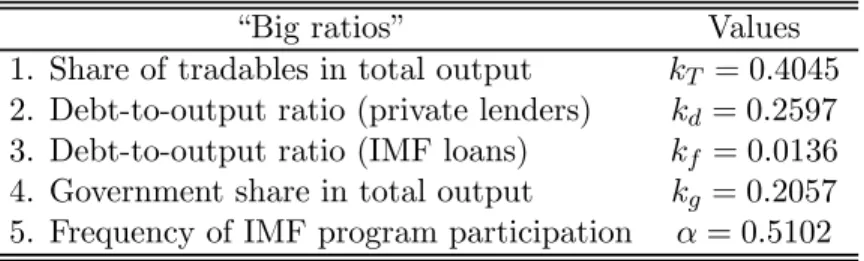
Table 1: Targeted Average Long-Run Ratios
“Big ratios” Values
1. Share of tradables in total output kT = 0.4045
2. Debt-to-output ratio (private lenders) kd= 0.2597
3. Debt-to-output ratio (IMF loans) kf = 0.0136
4. Government share in total output kg= 0.2057
5. Frequency of IMF program participation α= 0.5102
The calibration procedure (see Appendix B for a more detailed description) takes as reference a long-run situation in which E(zt) = 0 and the values of the tradable endowment and the real
exchange rate are normalized to yT = p= 1. Let variables without the time subscript,t, indicate long-run averages and letY =¡yT +pyN¢, the total endowment in units of tradable goods, be the
model’s proxy for total output. We targetfive long-run ratios: (1) the average share of the tradable output in total output,kT =yT/Y; (2) the average debt-to-output ratio from bank loans,kd=d/Y;
(3) the average debt-to-output ratio from Fund loans, kf = f /Y; (4) the ratio of government
spending (as a proxy for total consumption of public goods) to total output,kg =
¡
gT +pgN¢/Y; and (5) the frequency with which the economy participates in an IMF program,α. Table 1 shows the long-run ratios computed from Brazilian data.19
1 9
Data on GDP, tradable GDP (proxied by the GDP excluding the sum of before-taxes GDP for services and the construction industry, plus afinancial dummy), and government spending were obtained from the Instituto Brasileiro de Geografia e Estatística (IBGE). Total external debt corresponds to the net external debt (external debt minus
Exploring the recursive formulation of the central planner’s problem, a numerical solution is ob-tained using the value function iteration method, with discretization of the state-spaceS. The dis-crete grids used to represent the continuous supports ford∗t,zt, andftcontain602,5, and2points,
respectively. Thed∗
t grid implies debt-to-output ratios approximately in the range[−0.4,2.83], and
is appropriately chosen to include the ergodic space. The stochastic process for the production shock mimics a first-order autoregressive process of the type zt= ρzt−1+εt, with εt vN(0, σε),
ρ= 0.7188, and σε = 0.0229, and it is discretized into a five-point Markov chain using Tauchen’s
(1986) procedure.20
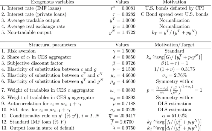
Table 2: Summary of the Calibration Procedure
Exogenous variables Values Motivation
1. Interest rate (IMF loans) r∗ = 0.0081 U.S. bonds deflated by CPI
2. Interest rate (private loans) r= 0.0282 C Bond spread over U.S. bonds
3. Average tradable output yT = 1.0000 Normalization
4. Average real exchange rate p= 1.0000 Normalization
5. Non-tradable output yN = 1.4722 kT =yT/
¡
yT +pyN¢
Structural parameters Values Motivation/Target
1. Risk aversion γ= 1.5000 Standard
2. Share ofct in CES aggregator δ= 0.9850 kg ∼=avg
£
Gt/
¡
yTt +ptyN
¢¤
3. Subjective discount factor β = 0.9726 β(1 +r) = 1
4. Elasticity of substitution between cand g ν = 2.1500 1/(1 +ν) = 0.3175
5. Elasticity of substitution between cT and cN µ
c= 4.6600 σy = 2.76%
6. Elasticity of substitution between gT andgN µg = 4.6600 Symmetry withc 7. Weight of tradables in CESc aggregator ωc= 0.0893 p= (1−ωωcc)
³
cT
cN
´(1+µc)
= 1
8. Weight of tradables in CESg aggregator ωg = 0.0893 Symmetry withc
9. Autocorrelation forzt=ρzt−1+εt ρ= 0.7188 OLS estimation
10. Std. dev. forzt=ρzt−1+εt σε= 0.0229 OLS estimation
11. Conditionality rule on gi ¡%yi¢,i=T, N gi = 20.9417 α= 51.02%
12. Standard IMF loan (%Y) f = 2.6700 kf ∼=avg
£
ft/
¡
yTt +ptyN
¢¤
13. Output loss in state of default λ= 0.9750 kd∼=avg
£
dt/
¡
yTt +ptyN
¢¤
As previously noted, the assumption that r > r∗ ensures ft = f whenever IM Ft = 1, which
allows the use of the two-point grid©0, fªand substantially reduces the dimension of the state-space and the computational cost of the numerical solution. The economy gets ft= 0when the planner
chooses IM Ft = 0, and a standard loan, f, whenever IM Ft = 1. The value of f is calibrated to
match the average value of IMF loans as a proportion of the GDP observed in Brazil.21 Table 2
international reserves) for the period 1982Q4−2004Q2 and is available from the Banco Central do Brasil. IMF loans and country participation in IMF programs were obtained from the IMF. In computingkd,“private loans” are simply
all outstanding external debt not contracted from the IMF, and may include other sources than private banks, such as loans from the World Bank and other multilateral agencies.
2 0
The points in the gridΩhZ={z1, ..., z5}are such thatytT>0at all times.
2 1It also satisfies the conditiond∗
displays the calibrated values of the remaining exogenous variables r, r∗, yN, and gi, i= T, N, and structural parametersγ,δ,β,ν,µc,µg,ωc,ωg, and λ.
The algorithm used in the numeric solution is the following. For each iteration j, given the discretized state-space and an initial guess for the borrowing constraint, d∗(j), the unconstrained model (no borrowing constraint) is solved and value functions VD(j)(z
t) and VR(j) ³ d∗ t−1,Sbt ´ , as well as the decision ruled∗(j)¡d∗t−1, St
¢
, are computed through iteration on the Bellman equation.22 During this step, the borrowing constraint is imposed, meaning that whenever d∗(j)¡d∗t−1, St
¢
is such thatd∗(j)> d∗(j), we setd∗(j)=d∗(j). Updates of the borrowing constraint are obtained using the following: d∗(j+1) = min h ΩZ n d∗(St) :VR(j) ³ d∗(St), St ´ =VD(j)(zt) o . The procedure is implemented until convergence when d∗(j+1) ≈d∗(j).
3.1
Results
Tables 3 and 4 show the average results of500simulations of a time series of98quarters, correspond-ing to the 1980Q1−2004Q2 period. The actual Brazilian series for private consumption, government consumption, and GDP, expressed in per capita values at average prices of 1991Q1, are taken from the Instituto de Pesquisa Economica Aplicada (IPEA), available at http://www.ipeadata.gov.br. They are consistent with data from the International Monetary Fund’s International Financial Statistics when they happen to overlap. Data on external debt and GDP in U.S. dollars, used to compute debt-to-GDP ratios, are obtained from the Banco Central do Brasil. Both the actual and simulated series for consumption and GDP are transformed previous to the computation of their second-moment statistics, as follows. First, all the variables are expressed in logarithms. Second, for the actual series, a seasonal adjustment on the log-variables is implemented using the multiplicative ratio-to-moving-average method. Finally, a smooth trend is subtracted by using the Hodrick-Prescott (HP)filter with a smoothing parameter of 1600.
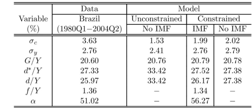
Table 3: Results I
Data Model
Variable Brazil Unconstrained Constrained
(%) (1980Q1−2004Q2) No IMF IMF No IMF
σc 3.63 1.53 1.99 2.02 σy 2.76 2.41 2.76 2.79 G/Y 20.60 20.76 20.79 20.78 d∗/Y 27.33 33.42 27.52 27.38 d/Y 25.97 33.42 26.17 27.38 f /Y 1.36 − 1.34 − α 51.02 − 56.27 −
2 2This step itself requires initial guesses for the value functions, and the iterations on the Bellman equation are
In general, the baseline model calibration of a borrowing-constrained economy with the option of seeking the IMF’s assistance is able to match the data well. Note that the calibration implies good approximations to the debt-to-output ratios (both from private lenders and from the IMF), the consumption of public goods as a proportion of the GDP, and Brazil’s participation in IMF programs.
In Table 3,σcandσyrepresent the volatility of (the log of) total private goods consumption and
total GDP, in units of tradable goods, as given byCt=cTt +ptcNt andYt=yTt +ptyN, respectively.
Note that the comparison between the constrained and unconstrained economies shows that the borrowing constraint increases consumption and GDP volatility from 1.53 per cent and 2.41 per cent, respectively, in the unconstrained economy (with no IMF), to1.99per cent and2.76per cent in a constrained economy when the Fund is present, and to2.02per cent and2.79per cent when it is not. That is, given that the economy faces a borrowing constraint, the IMF means less volatility. Although the model generates a higher relative consumption volatility (72.1per cent) in compar-ison with the unconstrained economy without the IMF option (63.5 per cent), it cannot reproduce the absolute level of consumption volatility observed in the data. This is a shortcoming, because consumption is more volatile than output in emerging economies (Resende 2006), which means that other sources of consumption volatility may be missing from the analysis, such as interest rate shocks (Neumeyer and Perri 2004) or permanent shocks to the growth rate of productivity (Aguiar and Gopinath 2004), as well as commodity-price shocks and the lack of well-developed domestic credit markets for households.23
The comparison between the constrained economies with and without the IMF seems to suggest that IMF loans crowd out private loans, having a negative catalytic effect. In Table 3, note that, despite the small increase in total debt when the IMF is present, the amount of private loans is higher with no IMF, and the difference is almost totally accounted for by Fund loans. Nevertheless, even though private loans behave as substitutes for Fund loans (rather than as complements to them), the country’s access to international capital markets is indeed facilitated by the Fund, because the direct effect of IMF lending makes the borrowing constraint ontotal debt less stringent (Table 4).
Potentially, the increase in available funds for the country to borrow, in the model, may come from two sources. First, there is the direct increase due to the possibility of borrowing from the Fund, given the maximum amount of private loans. Second, there is the possibility that the borrowing constraintd∗t may be positively affected by a general-equilibrium effect of the country’s decision to join an IMF program, when this decision reduces the likelihood of default on the external debt. If the borrowing constraint on private loans,d∗t−f, turns out to be higher than it would be 2 3I thank Larry Schembri and Robert Lafrance, of the Bank of Canada, for suggesting these two other potential
in the absence of the IMF, then there is positive catalysis of private capitalflows by IMF lending. In the above exercise, the opposite situation is observed (Table 4), sinced∗t−f is lower for the case with IMF, regardless of whether the economy is participating in an IMF program at periodt−1.
Table 4 shows that, considering the triplet ¡IM Ft−1, ft−1, gi
¢
, there is no difference in d∗t be-tween the model without the IMF and the model with the IMF when IM Ft−1 = 0.24 However,
the borrowing constraint on total debt is less stringent when IM Ft−1 = 1. Given the country’s
participation in IMF programs reported in Table 3, this means that in56per cent of the time, the economy has more room for consumption smoothing than it would if it did not have the option of seeking the Fund’s assistance. In the constrained economies, as shown in Table 3, the lower volatil-ity associated with the presence of the IMF is a result of this less stringent borrowing constraint. This also explains why the borrowing constraint binds less frequently in the IMF case, as shown in Table 4.25 Table 4: Results II ft−1 gi d∗t d ∗ t−f Bindingd ∗ t Model IM Ft−1 (% GDP) ¡ %yi¢ (% GDP) (%GDP) (%) Constrained No IMF − 0.0 ∞ 77.79 77.79 0.63 Constrained 0 0.0 ∞ 77.89 75.30 0.58 IMF 1 2.59 20.94 79.07 76.48
Figure 2 shows how the baseline model changes when the conditionality rule on gi becomes less stringent. In all four graphs, from left to right, the caps gi, i = T, N imposed by the IMF are relaxed. Notice that, as conditionality is just slightly stronger (i.e., gi is reduced by less than
0.012per cent of the GDP) than our baseline case, IMF participation and IMF lending (upper left corner) are null. As we move to the right, and conditionality is relaxed, IMF participation and IMF lending increase, reducing the volatilities ofCand Y (upper right corner), as well as the frequency with which the borrowing constraint binds (lower left corner).
The negative catalysis of IMF lending can also be seen in the lower right corner of Figure 2. Since the averaged∗
t/Ytis relatively unaffected asgi increases, the higher averageft/Ytmeans that
the average borrowing from private banks must be reduced. That is,dtis crowded out byftbecause
of the substitution of loans from private banks by cheaper loans from the IMF, as conditionality is relaxed and the economy’s total borrowing needs are relatively unchanged.
2 4
In the percentage of the GDP, the small difference is due to effects of the real exchange rate on the total GDP. The levels ofd∗t are the same in both cases.
2 5
The debt limit as a proportion of the simulated average GDP, both with and without the IMF, is such that it corresponds to more than the lower bound of47 per cent, given by the maximal level for the debt-output ratio observed in Brazil, over the period 1980Q1−2004Q4.
Volatility (%) 2.75 2.76 2.77 2.79 2.80 2.81 20.930% 20.940% 20.942% IMF conditionality 1.98 2.00 2.02 2.03 2.05 2.07 Y C
IMF Loans (% GDP) and IMF Participation (%)
0.00 0.30 0.60 0.90 1.20 1.50 20.930% 20.940% 20.942% IMF conditionality 0.0 12.0 24.0 36.0 48.0 60.0 f / Y Freq. IMF Bind (%) 0.50 0.54 0.58 0.62 0.66 0.70 20.930% 20.940% 20.942% IMF conditionality External Debt (% GDP) 26.0 26.4 26.8 27.2 27.6 28.0 20.930% 20.940% 20.942% IMF conditionality d*/Y d/Y
Figure 2: Effects of Changes ingi
It is important to understand why IMF lending does not catalyze private loans in this set-up. In general, positive catalysis of private lending occurs when there is a reduction in the likelihood of default induced by the IMF programs. If they can reduce the incentives of default, foreign lenders may relax their borrowing constraint. Strictly in terms of IMF lending, abstracting from the conditionality aspect of adjustment programs, its effect on the likelihood of default is ambiguous because of the lower interest rate charged on IMF loans, as explained in section2.6.
As for the effect of IMF conditionality on positive catalysis, it depends on how much it increases the economy’s ex ante propensity to save. To the extent that highly indebted economies can benefit more, instantaneously, from the higher current consumption that can be achieved in case of default, higher propensity to save and lower demand for debt means less incentive to default. Figure 3 illustrates how the ability of IMF conditionality in stimulating savings and program participation depends on the structural parameters.
To better understand this point, first note that the consumption of private goods is a strategic complement (substitute) to the consumption of public goods whenever1 +ν is higher (lower) than γ. That is, if the elasticity of substitution betweencandgis lower than the intertemporal elasticity of substitution, then the marginal utility of cit is increasing in git, for i=T, N, implying that the consumption of public and private goods must change in the same direction. For the calibrated values used in the exercise, the relevant case is that of complementarity betweencand g.
Second, let giN o IM F¡d∗t−1, zt
¢
, i = T, N, be the decision rule that determines the optimal consumption of public goods in the case with no IMF. If the IMF imposes caps gi such that giN o IMF¡d∗t−1, zt
¢
a welfare cost of satisfying the IMF conditionality rule, since compliance implies suboptimal git. Agents can always substitute the (forced) reduction in their consumption ofgit by consuming more cit, but there is a misallocation cost. On the one hand, when private and public goods are closer substitutes, this cost is lower and the relative incentives to adopt an IMF program are larger, but conditionality is not likely to increase savings and, as a consequence, the catalytic effect is not likely to occur. This is also true if the weight ofgt in the CES consumption aggregator is small.
Highεc,g, δ and lowεt,t+1:
• c and g are strategic substitutes and/or g is not very important for overall utility;
• lower cost of suboptimal gi;
• more incentives to sign an IMF program;
• small ex ante increase in savings;
• small reduction in the likelihood of default;
• IMF lending is likely to take place, but with No catalytic effect.
Lowεc,g, δ and highεt,t+1:
• c and g are strategic complements and/or g is important in overall utility;
• higher cost of suboptimal gi;
• less incentives to sign an IMF program;
• higher ex ante increase in savings;
• greater reduction in the likelihood of default;
• IMF lending not very likely (prohibitive costs); catalytic effect unobservable.
IMF Conditionality and Structural Parameters
Elasticity of substitution between c and g: εc,g = 11+ν
Intertemporal slasticity of substitution between c and g:εt,t+1 = 1γ Share of ctin the CES aggregator:δ
Figure 3: IMF Conditionality, Forced Savings, and the Catalytic Effect
On the other hand, complementarity betweencandgimplies that the lower level ofgi
t, compared
with the case of no IMF, must be followed by a corresponding lower level of cit. If the resulting oversaving is too costly for the country, it tends not to go to the IMF for assistance. As Figure 2 shows, the country always chooses IM Ft = 0when gi is set too low. Of course, where there is no
IMF program participation, the catalytic effect is unobservable.
Consider the opposite situation, such that gN o IMFi ¡d∗t−1, zt¢< gi. Conditionality is “soft” and
IMF participation will be positive for somegi, since the constraintgit≤gi will not be binding and, at the same time, the country can still enjoy the benefits of cheaper IMF loans in case of need. In this situation, conditionalityis nota real cost for the country, because optimalgtiis always achieved without violating the IMF conditionality. However, the country is not forced to save more (than it would do freely) and, as a consequence, for each realization of the shock there is no reduction in
the likelihood of default and no positive catalytic effect takes place. On the contrary, the cheaper IMF lending compared with that of the private banks, combined with a non-binding conditionality rule, will induce the economy to consume more of both private and public goods. In particular, this is true for tradable goods, which leads to higher demand for external debt, forces private banks to be even more strict in their lending, and explains the negative catalytic effect on private lending reported above.
3.2
IMF programs as commitment devices
Consider a set-up, in which the planner does not choosegti optimally. Instead, the consumption of public goods can take only two values, gi
t ∈ © gi L, gHi ª ,i=T, N, where gi
L < giH, and the country
cannot commit to the low level of consumption of public goods,gi
L, even if it would be better for the
representative agent to do so. In addition, assume that IMF programs can act as a commitment device that allows the country to choose gti = giL. That is, when the economy is not formally under an agreement with the IMF, it must choose git = gHi , because it cannot commit with the low-spending regime, and by adopting a program the planner would be forced to choosegLi, because of conditionality.
The above assumptions can be motivated by the idea that the IMF can affect the domestic political game in such a way that provides incentives for the country to implement “good” policies. For example, Corsetti, Guimarães and Roubini (2004), in discussing the IMF’s role as international lender of last resort, cite two possibilities: (i) the conventional view on debtor moral hazard, whereby the IMF’s assistance reduces the incentives for costly but socially desirable policies if it insulates the economy from crises, or (ii) the alternative view that some governments may be willing to undertake the domestic political cost of adjustment macroeconomic policiesonly because
the IMF’s assistance improves their chances of success. See also Marchesi and Thomas (1999) and Morris and Shin (2005).
Formally, in this alternative set-up, the planner’s problem is identical to the original, as de-scribed in the previous section, except for conditionality rules (10) and (11). Given the new assumptions, those rules change into:
ifIM Ft = 0 :θt=θ0= © DEFt∈{0,1};dt∈D;ft= 0;gti =giH< yit,i=T, N ª , (15) ifIM Ft = 1 :θt=θ1= © DEFt= 0;dt≥0;0≤ft≤f <∞;git=giL< giH,i=T, N ª .(16)
Note that, if we consider the situation where giN o IM F¡d∗t−1, zt
¢
< gLi < gHi , then the reduction from giH togiL as part of IMF conditionality will force the country to save more and, at the same time, push the country closer to what would be the optimal level of gi
t. In this case, the catalytic
effect follows through, as shown in Tables 5 and 6. These tables display similar information to Tables 3 and 4, respectively, but the results are derived using the modified model with the same
basic calibration described previously for the original model. All parameters are the same, the only difference being that, instead of calibrated values for the caps gi, i =T, N, we have to calibrate values for the exogenous levelsgHi and gLi.
For this calibration, let kgj be the average ratio of consumption of public goods to GDP when
IM F =j, for j = 0,1. In addition, let κ be the average reduction in the consumption of public goods as a percentage of the GDP required by IMF programs, implying that kg0 = kg1+κ > k1g. According to Killick, Malik, and Manuel (1995), the average reduction in government spending in IMF borrowers, when comparing before and after an IMF program, is approximately 1 per cent of the GDP. Given κ = 0.01, we calibrate kg0 in order to approximate the target α = 51.02 per cent for program participation. The resulting calibrated values for the exogenous consumption of public goods are gHi =k0gyi = 0.2131 when IM Ft= 0, and giL =kg1yi = 0.2031 when IM Ft = 1,
fori=T, N.
Table 5: Results III (Alternative model) Calibration: gHi /yi = 21.3%;giL/yi= 20.3%
Data Model
Variable Brazil Constrained
(%) (1980Q1−2004Q2) IMF No IMF σc 3.63 2.39 2.57 σy 2.76 3.14 3.21 G/Y 20.60 20.81 21.32 d∗/Y 27.33 28.81 22.25 d/Y 25.97 27.32 22.25 f /Y 1.36 1.49 − α 51.02 51.23 −
Table 5 shows that, compared with the model with no IMF, the presence of the Fund implies: (i) a lower ratio of consumption of public goods to GDP, as required by IMF conditionality; (ii) a higher total external debt as a percentage of the GDP, as in the original model; (iii) lower volatilities,σcand σy; and, most importantly, (iv) a higher level of private loans as a proportion of
the GDP, suggesting a positive catalytic effect of IMF lending that improves the country’s access to international private loans (not only to total loans).
Table 6: Results IV (Alternative model)
ft−1 gi d∗t d ∗ t−f Bindingd ∗ t Model IM Ft−1 (% GDP) ¡%yi¢ (% GDP) (%GDP) (%) Constrained No IMF − 0.0 21.3% 79.56 79.56 0.36 Constrained 0 0.0 21.3% 83.96 81.33 0.31 IMF 1 2.63 20.3% 85.95 83.33
Table 6 show evidence of the positive catalytic effect of IMF lending in this modified mode. Note that not only is the borrowing constraint for the total external debt higher when the IMF exists, but so is the borrowing constraint on private loans,d∗t−f. As a consequence, the borrowing constraint binds less frequently in the model with the IMF.
The mechanism through which the positive catalysis takes place is based on the increase in the country’s external payments position due to IMF conditionality that forces the country to adjust (reduce) its level of consumption of public goods from giH to gLi. Since the consumption of private goods is not a perfect substitute for the consumption of and public goods, and given that agents care about their future levels of consumption, the reduction in gt forces the country to
save more. By locking countries into a program of reform that ultimately improves their external payments position, conditionality provides external investors and private banks with a high degree of assurance about the country’s decision to repay past debt instead of defaulting. Thus, ceteris paribus, the reduced likelihood of default allows private banks to relax the borrowing constraint.
To summarize the results so far:
1. IMF lending helps relax the borrowing constraint on total debt and, as a consequence, reduces the volatility of private consumption and GDP.
2. When countries optimally choose their allocations of public goods, then IMF conditionality, based on restraining the consumption of public goods, does not catalyze private capitalflows: when conditionality imposes a real cost in terms of suboptimal higher savings, countries choose not to sign IMF programs; when conditionality is not binding, countries will sign IMF programs but will not be forced to save more.
3. When countries use the IMF as a commitment device to reduce their spending on public goods, then IMF conditionality forces a higher level of savings, reduces the likelihood of default, and allows private banks to be less strict in their lending, which produces the positive catalytic effect on private loans, as the Fund claims.
The remaining question is: by how much does a less stringent borrowing constraint, due to the direct effect of IMF lending and/or a positive catalytic effect induced by conditionality, improve welfare?
3.3
Welfare analysis
In terms of the welfare implications of IMF programs, there are two forces at play. The potential cost of adopting a program is a requirement to adjust the country’s domestic absorption to the conditionality clauses, meaning that the country has to face constraint (11)−and set gTt and gtN at potentially suboptimal levels−or rule (16), in the case of the alternative model. The benefits,
besides the lower interest on IMF loans, are related to the additional amount of external funds available for borrowing, on top of dt, which will allow a higher degree of consumption smoothing.
To assess the welfare effects of IMF-supported programs, the consumption-equivalent approach is used. In particular, we compute the per cent increase in consumption across dates and states, such that the representative agent would receive the same utility, considering worlds with and without the IMF. Let ϑ be this equivalent variation in consumption allocations, and let the superscripts
IMF and N o IM F indicate the utility functions and value functions for the equilibrium values of
consumption in worlds with and without the IMF, respectively. The value of ϑ can be computed
from: Z S E0 ∞ X t=0 βtuIM F ¡qcTt, qctN, qgtT, qgNt ¢dφ= Z S0 V0N o IM F dφ0, (17) where V0N o IM F = E0P∞t=0βtuN o IM F ¡
cTt, cNt , gTt, gtN¢ is the value function obtained under the assumption that there is no IMF in the world, and q= 1 +ϑ.
The sets S andS0 are the supports for the state of the economy in worlds with and without the IMF, respectively. Note that the IMF is welfare improving in the case that q < 1, meaning that the consumption in a world with the option of joining an IMF program has to be decreased by ϑ in order to generate the same level of welfare as that of a world without the IMF.
In the quantitative exercise, using the original model presented in section 2 to compare two economies that are identical except for the fact that one operates in a world with the IMF and the other in a world without the IMF, q is found to be equal to 0.9903. That is, in order to match the same welfare obtained in a world where there is no option of seeking the IMF’s assistance, the consumption sequence observed in a world with the IMF has to be decreased by 0.97 per cent. In the alternative model, with no optimal choice of consumption of public goods, we find that q = 0.9958, implying a 0.42 per cent reduction in consumption required to compensate for the lower welfare observed in the same economy if it does not have the option of seeking the IMF’s assistance. Therefore, results suggest that the IMF has an overall small positive effect on welfare.
4
Conclusion
This paper has presented a dynamic model of an endowment, two-goods, small open economy subject to an endogenous borrowing constraint, where the planner can optimally choose to join an IMF-supported adjustment program. The quantitative exercise consisted of a comparison between one economy, which has the option of seeking the IMF’s assistance, and another economy, identical in all aspects to the first except that there is no IMF in the world (the counterfactual). The paper provides answers to two questions. First, can IMF conditionality, focused on the control of the consumption of public goods, generate a positive catalytic effect, as the Fund claims? Second, what is the welfare gain associated with IMF programs?
In terms of the numeric results, the answer to the first question depends on whether IMF conditionality can force the country to save more while offering enough compensation for these additional suboptimal savings that the country can actually decide to sign an IMF program. If the consumption of public goods is chosen optimally by the central planner, then whenever the conditionality rule is too strict (relative to the optimal level for the no-IMF case), the country will not participate in IMF programs. The oversaving implied by conditionality is too costly for the economy.
On the other hand, when conditionality clauses are redundant (because the country’s optimal consumption of public goods is lower than the level determined by conditionality), not forcing the economy to save, then IMF participation is positive, but there is no improvement in the prospective for repayment of the external debt by the borrowing country. It is the opposite: since conditionality is not a real cost and the country can still borrow at a lower interest rate from the IMF, private banks must be more strict to avoid default. This generates a negative catalytic effect of IMF lending on private capitalflows, although the borrowing constraint on total external debt may be relaxed. Only by increasing a country’s external payments position may the Fund help the country signal to foreign private lenders that the opportunity cost of defaulting has become higher, and the likelihood of debt repudiation reduced. This, in turn, allows international private creditors to relax their borrowing constraint. This situation can occur when the planner does not optimally choose the allocations of consumption of public goods. In that case, under the assumption that the IMF can act as a commitment device that allows the economy to operate with a lower level of consumption of public goods than it would otherwise, IMF conditionality produces a positive catalytic effect on private capital flows. Catalysis occurs because the reduction in consumption forces the country to save more and, at the same time, pushes the economy closer to what would be the optimal allocation. As a result, the likelihood of default is reduced and private banks can relax their borrowing constraints. Both the direct (additional source of loans) and indirect (positive catalysis on private loans) effects of IMF lending imply a less stringent borrowing constraint that allows more room for consumption smoothing.
A less stringent borrowing constraint, however, resulting from either direct lending or positive catalysis of privateflows, is not a measure of the “success” or “failure” of IMF programs. The welfare effects associated with IMF lending do not seem to be very quantitatively important. It is true that the less stringent borrowing constraint allows the country easier access to international capital markets and, as such, improves the country’s consumption-smoothing opportunities. The reduction in volatility does produce welfare improvements, but for the parametrization used in the calibration exercise, which was set to approximate the Brazilian economy during the 1980Q1−2004Q2 period, IMF lending generates improvements in welfare equivalent to less than 1 per cent in additional consumption.
References
Aguiar, M. and G. Gopinath. 2006. “Defaultable Debt, Interest Rates and the Current Account.”
Jounal of International Economics 69(1): 64−83.
Aiyagari, S.R. and M. Gertler. 1991. “Asset Returns with Transactions Costs and Uninsured Indi-vidual Risk.”Journal of Monetary Economics 27: 311−31.
Arellano, C. 2004. “Defaultable Risk, the Real Exchange Rate and Income Fluctuations in Emerging Economies.” Society for Economic Dynamics Meeting Paper No. 516.
Barro, R.J. and J.W. Lee. 2005. “IMF Programs: Who Is Chosen and What Are The Effects?”
Journal of Monetary Economics 52(7): 1245−69.
Bird, G. 1996. “Borrowing From The IMF: The Policy Implications of Recent Empirical Re-search.”World Development 24(11): 1753−60.
Bird, G., M. Hussain, and J.P. Joyce. 2004. “Many Happy Returns? Recidivism and the IMF.”
Journal of International Money and Finance, 23: 231−51.
Bird, G., A. Mori, and D. Rowlands. 2000. “Do The Multilaterals Catalyze Other Capital Flows? A Case Study Analysis.” Third World Quarterly 21(3): 483−503.
<