Aggregate Queries in NoSQL Cloud Data Stores

(1)

Aggregate Queries in NoSQL Cloud Data Stores

Master’s Thesis, PDCS

Submitted to the Department of Sciences, Vrije Universiteit, Amsterdam,

The Netherlands

Plamen Nikolov (2000229) August 2011

Guillaume Pierre Principal Advisor

(2)

(3)

Abstract

This thesis work describes the design and implementation of an aggregate view mainte-nance mechanism for web applications in the Cloud. Maintaining consistent views and ensuring fault and partition tolerance is generally hard as the CAP theorem postulates that these three properties cannot hold simultaneously. Nevertheless, web application transac-tions are often characterized by short-lived transactransac-tions touching only a few data items. Specific examples are shopping cart updates, user name and password look-ups, and online visitor statistics. The small sized updates allow for an efficient aggregate view maintenance solution based on incremental updates via change tables. The change table mechanism can be readily implemented at a transaction coordinator node which can carry out the entire computation because of the small-sized view change tables.

This thesis elaborates on using the two-phase commit protocol and simple equi-join queries to implement a synchronous and asynchronous version of the change table algo-rithm. In this work we will argue that the heavy workloads introduced by the synchronous approach can be decreased by relaxing the view freshness requirements. Thus, the perfor-mance of the proposed mechanism can be controlled by exploiting the whole consistency range from immediate updates to deferred refreshing which can be carried out at arbitrary time intervals.

(4)

List of Tables

2.1 Aggregate Query Row Access Counts . . . 11 4.1 Change Propagation Equations [15] . . . 22

(7)

List of Figures

1.1 LinkedIn and WordPress Platform monthly traffic measured in people per

month (Source: Quantcast.com) . . . 2

1.2 Data Flow within a Web Application . . . 4

1.3 Aggregate View Maintenance via Summary Tables . . . 6

2.1 Web Application Accounting for User Clicks and Page Views . . . 9

2.2 SQL Query Plan . . . 10

2.3 Data Cube . . . 12

3.1 MapReduce Framework . . . 15

4.1 Change Table Derivation after a Base Table Update . . . 21

5.1 CloudTPS Architecture . . . 24

5.2 Synchronous Computation Two-Phase Commit Protocol . . . 28

6.1 Aggregate View Maintenance Experimental Setup . . . 32

6.2 Performance Evaluation of the Synchronous and Asynchronous View Maintenance Algorithms (transactions per second vs update size) . . . 33

6.3 Asynchronous View Maintenance with Different Refresh Frequencies (transactions per second vs update size) . . . 34

6.4 Performance Evaluation of the Synchronous View Maintenance Algorithm with TPC-W (transactions per second vs update size) . . . 35

(8)

Chapter 1 Introduction

1.1 From Relational Databases to NoSQL

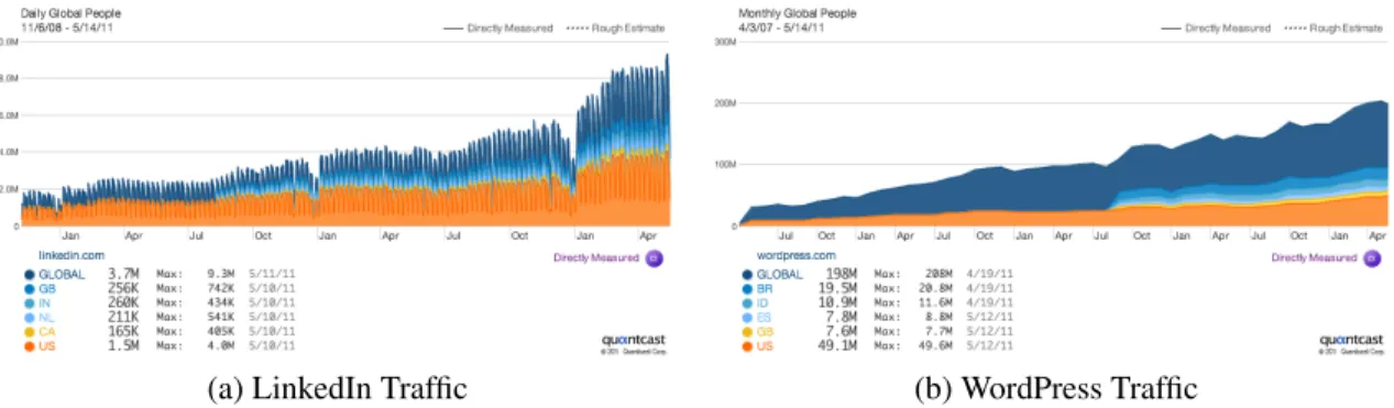
According to Moore’s law transistor density doubles every two years while semicon-ductor prices decrease steadily [19]. The exponential growth in computer power and cost-performance ratio has led to an increased availability of commodity computers and widespread usage of cluster and on-demand computing on the Cloud. The shift from ex-pensive state-of-the-art machines to inexex-pensive commodity hardware necessitates rethink-ing web application models from resource provisionrethink-ing to storage engines in order to allow for user base expansions and handling hardware failures in a distributed environment. With the increase of computational power, the application’s user base grows as well (Figure 1.1), challenging web services with millions of users demanding low response times and high availability. As in reality users increase asymptotically faster than transistor density, sys-tem architect wizards have to resort to increasingly sophisticated tricks in order to address the scalability issues in the data storage tier.

Generally, database scalability can be achieved by either vertically or horizontally scal-ing the database tier:

• Vertical Scalability: When scaling vertically, the database tables are separated across different database instances on potentially distinct machines so that each server is assigned a specific task. While this approach results in efficient I/O load-balancing, vertical scalability depends on the presence of logically separable compo-nents of the database and the ability to constantly upgrade the existing hardware; • Horizontal Scalability: When scaling horizontally, the database structure remains

unchanged across all the database instances. Achieving horizontal partitioning re-quires a consistent maintenance between the different instances and their replicas, efficient load balancing, and I/O aware query algorithms so that the data transfer

(9)

CHAPTER 1. INTRODUCTION 2

(a) LinkedIn Traffic (b) WordPress Traffic

Figure 1.1: LinkedIn and WordPress Platform monthly traffic measured in people per month (Source: Quantcast.com)

latency is minimized. Theoretically, the achieved database speed-up by horizontal scaling is proportional to the number of newly added machines.

For Cloud-based web-applications, vertical scalability is not a viable solution as it involves adding new resources to a single node in the system. While the prices of off-the-shelf com-ponents have radically decreased over the last several years, there is a limit to the number of CPUs and memory a single machine can support. Typically, systems are scaled vertically so that they can benefit from virtualization technologies; a common vertical scalability practice is placing different services and layers on separate virtual machines to facilitate migration and version management.

One of the biggest challenges facing web applications is not the lack of computa-tional power but efficiently and resiliently processing a huge amount of database query traffic [22]. More than 30 years old, RDBMSs represent the perfect storage solution on high-end multi-core machines equipped with enormous hard drives. With their impressive feature set, transaction management, and query capabilities relational database solutions are able to handle nearly any imaginable task. However, problems start arising once these databases have to become distributed in order to handle the more demanding traffic; coming from the era of mainframes, they were never designed to scale. Below are listed only some of the issues causing relational databases to lose the lead in large scale web applications:

• Behemothian data volumes require applying a heavy data partitioning scheme across a huge number of servers, also referred to as sharding1, leading to a degraded perfor-mance of table joins;

1_{A popular distributed database design is horizontal partitioning in which the database rows are distributed}

across different partitions. Each partition belongs to a shard which might be located on a different database server.

(10)

• Systems with heavyweight transaction management cannot handle efficiently con-current queries;

• Relational databases cannot handle efficiently data aggregation from large shard vol-umes due to high communication costs.

Many of the described scalability issues can be addressed by relaxing the consistency re-quirements and dropping the relational schema. This argument is especially pertinent to web applications as they exhibit a different data access behavior than enterprise data min-ing platforms. A typical model-view-controller web application uses a small subset of SQL with fine-grained data access patterns and performs very few writes compared to the num-ber of read operations. Thus, the data model can be readily expressed as key-value pairs or simple document corpora which can be accommodated by data stores such as Google’s BigTable [8], Amazon’s SimpleDB [3], and open-source projects such as HBase and Cas-sandra. These and other similar storage solutions go under the umbrella name of NoSQL.

1.2 Scalable and Consistent R/W and Equijoin Queries in

the Cloud

Currently most NoSQL databases provide extremely limited functionality as they do not support atomic updates, join, and aggregate query capabilities. Often when consistency is not a key requirement, porting the storage tier of an application from a relational database to a non-relational solution such as Hadoop only requires denormalizing the data model [7]. This is the case for applications using “approximate” information2(e.g. approximate num-ber of a website page views). On the other hand, there are many applications which cannot use a weak data consistency model. For example, overselling a physical item in an online store is a highly undesirable event at best.

Providing strong consistency in non-relational stores is generally a hard problem. Intu-itively, the distributed nature of the data results in a higher cost to synchronize all changes made by a transaction into a known single state. More formally, these challenges are cap-tured by Brewer’s theorem postulating the impossibility for a distributed system to simul-taneously provide consistency, availability, and partition tolerance [10]. Nevertheless, web applications exhibit certain data access patterns which ease the strong consistency problem. The CloudTPS middleware introduces a novel approach for achieving strong consis-tency in NoSQL by taking advantage of the short-lived, relatively small queries character-istic to web applications [23]. The proposed framework uses multiple transaction managers to maintain a consistent copy of the application data to provide developers with a means

2_{The database operations in the “approximate” reads scenario are not serializable. The final outcome is}

(11)

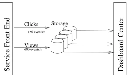
Service Front End

Dashboard Center

Clicks

Views

150 events/s

600 events/s

Storage

Figure 1.2: Data Flow within a Web Application

to create web applications by following common engineering practices instead of circum-navigating the peculiarities of NoSQL. For example, the TPC-W benchmark [18] can be implemented on CloudTPS with a minimum number of modifications [23]. However, CloudTPS lacks the implementation of an important query class–data aggregation.

1.3 Motivation

As data sets and user bases grow larger, so does the need for aggregate queries in the Cloud. For example, Wikipedia and the Wordpress platform already use extensively MIN-MAX queries. E-commerce web applications often provide real-time dashboards providing functionality from aggregating the contents of a shopping cart to displaying sophisticated analytics about clicks, impressions, or other user events. Figure 1.2 shows a simplified scheme of a large scale web application providing real time analytics for user events. With several hundred events per second, performing real time data aggregation using a relational database is an intimidating task due to the large number of write operations and reads spanning numerous shards.

Formally, data aggregate queries are defined as functions where the values of multiple rows are grouped together according to some criteria–a grouping predicate–to form a single value of more significant meaning. By far, the most popular aggregate functions in web applications are count, sum, average, minimum, and maximum over the result of a select-project-join (SPJ3) query:

• Count()returns the number of rows;

(12)

• Sum()returns the sum of all values in a numeric column;

• Average()returns the average of all values in a numeric column.

Currently none of the existing approaches for computing aggregate functions in the Cloud targets web applications using a generic data store. Instead, they exploit knowledge about the data model, compute the result offline, or take advantage of the functionality present in a specific data store; obviously, none of these approaches is applicable for the service described on Figure 1.2.

1.4 Aggregate Queries for Large-Scale Web Applications

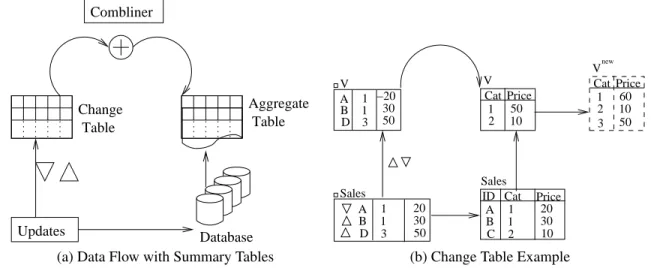
Many web applications such as Wikipedia, the WordPress platform, and the dashboard application from Figure 1.2 use short-lived transactions spanning only a few rows in the underlying data store. For example, in the dashboard application, each click results in the update of the rows corresponding to the page being viewed. The relatively small size of typical web application transactions allows the efficient maintenance of summary tables

containing the results of predefined aggregate queries. By using summary tables, incoming aggregation requests are served by simply looking up the result in the appropriate sum-mary table. Because the aggregation work has been delegated to the mechanism updating the aggregate summary tables, the data store can treat all incoming aggregate queries as simple read-only operations and take advantage of the underlying horizontal scalability. Intuitively, the data in the aggregate summary table can be incrementally maintained; for example, inserting a row in a table participating in aCOUNTquery may result in increasing the aggregate result. This approach is shown on Figure 1.3a:

1. Initially, the summary tables are directly computed from the data available in the application’s tables;

2. As updates, deletions, and insertions are coming in, the data store commits the mod-ifications and computes change tableswhich “describe” how the updates affect the summary tables; the new value of a summary table after an update is a function of the old value and of the data present in the change table;

3. The data store uses the change tables to update the aggregate summary tables. Figure 1.3b illustrates the change table approach for aggregate summary tables. Initially, theSales table contains three products which have been aggregated by category in tableV

(View). At some point, the data store receives a transaction containing one insertion and two deletions and computes the corresponding change table V. As deletion operations may decrease and never increase the number of rows participating in the aggregate result, the numerical attributes participating in the aggregation have been negated; as shown on

(13)

CHAPTER 1. INTRODUCTION 6 Updates Change Table Combliner Database Aggregate Table

(a) Data Flow with Summary Tables

B D A 1 1 3 30 50 −20 V B D A 1 1 3 20 30 50 Sales V Cat 2 1 50 10 Price Sales ID Cat B C A 1 1 2 20 30 10 Price Vnew Cat 2 1 60 10 Price 3 50

(b) Change Table Example

Figure 1.3: Aggregate View Maintenance via Summary Tables

the diagram,A’s price inV has been set to−20. It is easy to see howV describes the modifications which have to be applied toV in order to make the summary table become consistent with the updates: each row from V is matched with rows fromV according to the Category attribute and upon a successful match, the Price attribute is added to the aggregate result. A natural observation is that the described “matching” operation is equiv-alent to an inner join. Section 4 will provide a formal description of this approach.

The usage of change tables to maintain aggregate views has been studied extensively in the relational database world [1], [12], [14], [20], [21]. The strongly consistent read-only and read/write transactions in CloudTPS make the CloudTPS middleware suitable for implementing the summary table mechanism for aggregate queries. This thesis extends the change table technique to NoSQL data stores by adapting the view maintenance algorithm for usage in CloudTPS. The approach shown on Figure 1.3a can be naively implemented by merging the change and aggregate tables using only one server in the distributed environ-ment. Unfortunately, this centralized solution would require shipping the entire aggregate summary table and result in a high bandwidth usage and latency penalty.

A data store’s scalability can be captured informally by Amdahl’s law [4]. If P is the portion of a program that can be parallelized, the maximum achievable speedup byN

processors is 1

(1−P)+_NP. Intuitively, the naive solution to the aggregate view maintenance

problem can be naturally improved by parallelizing the combiner process presented on Figure 1.3a. As the aggregate view and change tables are automatically partitioned and replicated by the CloudTPS middleware, in the following sections we will concentrate on two view maintenance algorithms which generate the aggregate change tables and consis-tently update their corresponding views.

(14)

1.5 Thesis Structure

Before proceeding with the aggregate query algorithms and their implementation, we will start in Chapter 2 with a motivating example which will be used throughout this text. Chap-ter 3 will introduce several existing solutions to the aggregate problem and their shortcom-ings in the context of Cloud-based web applications. Next, Chapter 4 will review the theory behind the proposed solutions. Chapters 5 and 6 will deal with the actual aggregation algo-rithm implementation details and evaluation. Finally, Chapter 7 will recapture the aggregate view maintenance approach and provide a conclusion.

(15)

Chapter 2 Background

2.1 Motivating Example

As discussed in the introduction section, large-scale web applications exhibit a different behavior than data warehouse applications. Unlike large-scale enterprise OLAP (Online analytical processing) platforms, web applications have short-lived queries which often span only a few tables. The following example discusses a simple web application which will be used for illustrating some major points throughout this thesis.

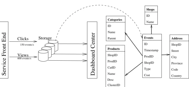
Figure 2.1 depicts the architecture of the accounting component of a simple e-commerce application which displays products and receives revenue for product views and clicks. Formally, the front end generates “click” and “view” events whenever a product is clicked and viewed respectively and updates a database. The application’s database has the following schema:

• Events(ID, Timestamp, ProdID, ShopID, Type, Cost) stores all user events. Each event is represented by a unique ID, a Timestamp indicating the time at which it occurred, the product’s and shop’s IDs (ProdID, ShopID), the event Type, and the Cost which will be charged to the shop’s account.

• Categories(Id, Name, Parent) organizes the available products into categories–books, videos, etc. Each category is represented by a uniqueID, Name (e.g. “books” and “videos”), andParentID used for generating a category tree.

• Products(ID, ShopID, CatID, Name) stores all available products. Each product is represented by its unique ID, the shop offering the product (ShopID), its category (CatID), Name and Description, and cluster (ClusterID) grouping products which are instances of the same product (for example, two books with the same ISBN would have different IDs and equal ClusterIDs).

(16)

CHAPTER 2. BACKGROUND 9

Service Front End

Dashboard Center

Clicks Views 150 events/s 600 events/s Storage Name ID Parent Categories Products ShopID ProdID CatID Name Desc ClusterID Events ID Timestamp ProdID ShopID Type Cost Shops ID Name Address ShopID Street City Province Code Country

Figure 2.1: Web Application Accounting for User Clicks and Page Views

• Shops(ID,Name) stores the shops advertising products via the service; each shop is uniquely identified by itsID.

• Address(ShopID, Street, City, Province, Code, Country) stores the physical location of each shop advertising products.

The web application features a “Dashboard Center” allowing various analytics queries. For example, an end-user can examine the number of clicks and views a given product or category received and the resultant revenue. If the back-end storage solution is a relational database, finding the cost a specific merchant accumulated for the product views belonging to some category can be accomplished by issuing the following query:

Listing 2.1: SQL-1

SELECT Sum( c o s t ) AS C o s t FROM D i s p l a y , M e r c h a n t , C a t e g o r i e s

WHERE D i s p l a y . m e r c h a n t I d = M e r c h a n t . m e r c h a n t I d AND C a t e g o r i e s . c a t I d = D i s p l a y . c a t I d AND C a t e g o r i e s . c a t I d = ’ b o o k s ’ AND

M e r c h a n t s . m e r c h a n t I d = ’ K i n o k u n i y a ’

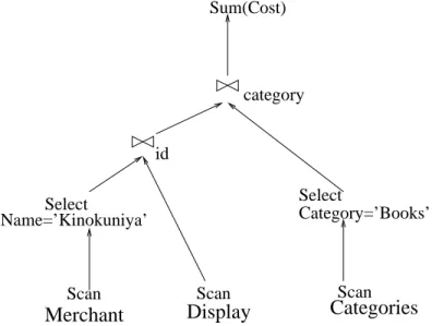
A typical query plan of the SQL query presented above is shown on Figure 2.2. In order to find the cost accumulated by the “Kinokuniya” shop in category “books”, the database scans the Merchant and Categories tables in order to retrieve the respective unique IDs. Next, the first join operator, denoted by./ID, outputs all rows from theDisplay table

cor-responding to products sold by “Kinokuniya”. The second join operator,./category, yields

all products belonging to the “Books” category. Finally, the result is summed over theCost

(17)

CHAPTER 2. BACKGROUND 10 Scan Display Categories Select Scan Select Name=’Kinokuniya’ Category=’Books’ Sum(Cost) Merchant Scan id category

Figure 2.2: SQL Query Plan

TheScan andJoin operations on Figure 2.2 exhibit data access patterns which have to be considered when looking into the performance of a Cloud implementation of the “Dash-board Center” web-application. In particular, the scalability of an application is largely influenced by the frequency at which it accesses different data items as well as by the physical data distribution across multiple hosts. The Scan operator makes only one pass through the table, emitting blocks matching the specified predicate. Moreover, the number of rows scanned is proportional to the table size. The asymptotic performance of theJoin

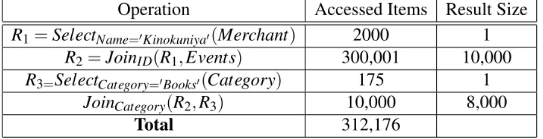
operator depends on the underlying database implementation. For example, a naive imple-mentation would compare each tuple from the outer relation with each tuple in the inner relation, resulting in a quadratic cost of the comparisons required. A more sophisticated approach, hash joining, requires reading the entire inner relation and storing it into a hash table which is queried for each tuple present in the outer relation. Nevertheless, in both cases each table row has to be accessed at least once, leading to complications in cases where the same query has to be repeatedly executed in a distributed environment, as we shall see shortly. Table 2.1 estimates the number of row accesses per operation in order to compute the aggregate query on Figure 2.2.

It is easy to see that the query shown on Listing 2.1 conforms to web-application query properties. First, it is short-lived as the query results needs to be delivered in “real-time”. Second, unlike enterprise data warehouse aggregations, the aggregation query plan does not involve sifting through terabytes of data.

The “Dashboard Center” described above is a typical relational database application with data flowing from an online transaction processing database into the data warehouse on an hourly basis. As evident from Table 2.1, even a simple aggregate query such as

(18)

Operation Accessed Items Result Size

R₁=Select_Name₌0_Kinokuniya0(Merchant) 2000 1

R₂=Join_ID(R₁,Events) 300,001 10,000

R3=SelectCategory=0Books0(Category) 175 1

Join_Category(R2,R3) 10,000 8,000

Total 312,176

Table 2.1: Aggregate Query Row Access Counts

the one shown in Listing 2.1 can generate a huge amount of traffic in a distributed en-vironment. Standard SQL solutions such as database mirroring and replication increase only the database’s availability but not its scalability. To deal with the latter problem, the database has to be partitioned horizontally. Horizontally partitioned tables distribute sets of rows across different databases often residing on different servers. This scheme decreases the level of contention between read and write operations at the expense of consistency and increased bandwidth requirement of composite queries such as the one used in the aggrega-tion example. The rest of the chapter will provide an overview of the available approaches to tackle the aggregation problem in the NoSQL world as well as their limitations.

2.2 Data Model

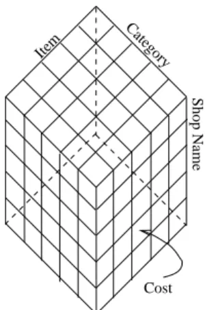
The data model used in Section 2.1 can be formally described via data cubes. In online analytical processing, a data cube defines the data model in several dimensions so that the stored information can be manipulated from different perspectives. There are two table types– dimension tables and fact tables. The former type stores non-volatile information while the latter represents time-variant data.

Figure 2.3 shows the data cube describing the data from the example in Section 2.1. As evident from the diagram, there are three dimension tables describing the information in terms of advertised items and their corresponding categories and sellers. Even though the data stored in these tables is not immutable, changes occur very rarely and are triggered by events such as user account creations or modifications. The facts from which the cost is computed are present in theEventstable which is periodically updated.

It is not difficult to see how data cubes can be used for web-application aggregate queries as measures can be performed at any dimension intersection. Informally, the cube dimensions are presented by theGROUP BY statement in SQL and the model can readily be applied for representation of totals such as the total sales from a specific category, web page visits by users from a given country, or the best performing seller for some product. The next few paragraphs will look into several existing ways in which this problem can be tackled.

(19)

Shop Name

2.3 Execution Environment

Unfortunately, computing the aggregate query shown on Listing 2.1 is far from trivial even with a modest amount of traffic such as several hundred views per second. The main reason for the poor performance is the fact that queries involving large tables requiring join and aggregate operations are expensive both in terms of computational cost and communication latency. As noted in Section 2.1, the system’s performance can be perceivably improved by scaling horizontally the application’s database tier. First, a very large fact table will be distributed across multiple servers, decreasing the workload on any specific instance. Second, the aggregate computation ideally is offloaded to multiple nodes. These two goals cannot be achieved by standard RDBMSs as their heavy-weight transaction handling re-sults in a poor performance and they cannot take advantage of the elasticity achieved by relaxing consistency requirements. The rest of this thesis will investigate data cube ag-gregate computations for web-applications using a key-value data store such as HBase for their database tier.

HBase is an open-source, distributed, large-scale, key-value data store based on Google’s BigTable. The data is organized in labeled tables; each data point is referred to as a cell. As cells are simple byte arrays, the data types widely used by RDBMS are eliminated and the data interpretation is delegated to the programmer. Each table cell is indexed by its unique row key and each row can have an arbitrary number of cells.

Intuitively, an HBase application has to use a data model resembling a distributed, sparse, multidimensional hash table. Each row is indexed with a row key, a column key, and a time-stamp. A table allows maintaining different data versions by storing any number of time-stamped versions of each cell. A cell can be uniquely identified by its corresponding row key and column family and qualifier, and time-stamp. The column keys are in the form

(20)

”family:qualifier”, where the family is one of a number of fixed column-families defined by the table’s schema, and the qualifier is an arbitrary string specified by the application.

It is easy to see why an HBase-like data store is suitable as the storage tier of a web application in the Cloud. New resources are automatically handled by the data store as all operations happen on a per row basis and theoretically, the data store can achieve un-limited horizontal scalability. Nevertheless, aggregate functionality cannot be implemented directly without a framework for breaking-up the queries so that local resources are utilized as much as possible without sacrificing bandwidth.

(21)

Chapter 3 State of the Art Data Aggregation for the

Cloud

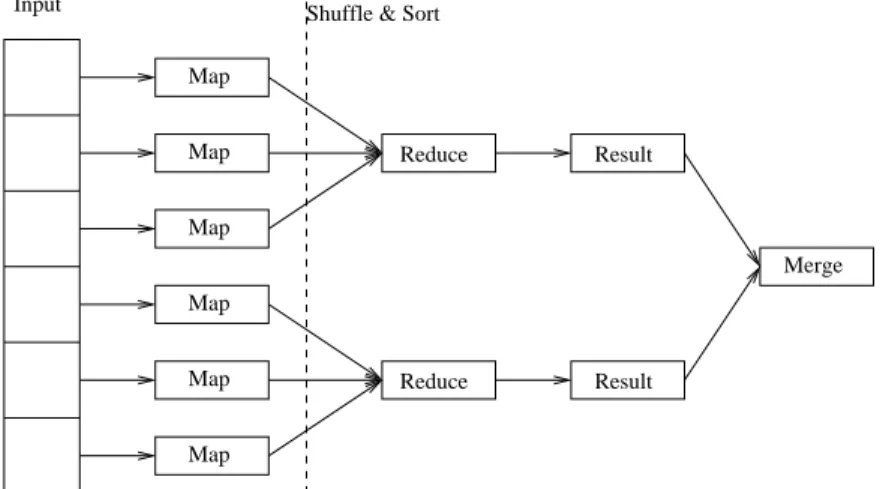
This chapter reviews the MapReduce framework which has been studied extensively and is widely used for large-scale data analysis. Even though, it can efficiently process terabytes of data, the MapReduce technique turns out to be unsuitable for web applications which often have to perform a set of predictable aggregations with low-latency requirements.

3.1 Aggregation with the MapReduce Framework

The MapReduce framework is used for large-scale distributed computation on computer clusters as well as on the Cloud. It can efficiently aggregate terabytes of data and yields in theory unlimited scalability. The model achieves massive parallelization by splitting the input into numerous pieces each of which is assigned to a computational node from the cluster (Figure 3.1). The map function runs on each node and emits key/value pairs. These are passed to the reduce function where the values are collated.

The MapReduce framework can be readily used for computing aggregate queries by using theMap and Reduce functions to build an execution plan equivalent to the original query. For example, the following SQL query,

SELECTCatId,SUM(Cost)FROMEventsGROUP BYCategory, can be computed in two phases as follows:

1. TheMap phase reads all records from the Category table and outputs records con-sisting of a "key", to which theCatId value is assigned, and "value", equal to "1". 2. TheReduce phase consumes the key-value pairs generated by theMap function and

aggregates them so that records with the same key occur together. TheReducephase accumulate all the 1’s to compute the final count.

(22)

CHAPTER 3. STATE OF THE ART DATA AGGREGATION FOR THE CLOUD 15 Map Map Map Map Map Map Reduce Reduce Result Result Merge

Input _{Shuffle & Sort}

Figure 3.1: MapReduce Framework

Moreover, if the aggregate query is commutative and associative, this approach can be fur-ther improved by computing in-network partial aggregtes–intermediate results which are combined to generate the final aggregation [24]. The following algorithm uses “com-biner” functions to generate the partial aggregtes within the MapReduce framework and is applicable toAverage,Count,Maximum,Median,Minimum, andSum functions [9]:

1. Map: applied on all input files to extract keys and records;

2. InitialReduce: operates on a sequence of records of the same type and with the same key to output a partial aggregation;

3. Combine: operates on a sequence of partial aggregations to output a combined partial aggregation;

4. Reduce: operates on a sequence of partial aggregations to compute the final aggre-gation result .

Based on the approach outlined above, any aggregate query can be expressed as: Listing 3.1: UsingMapReduceto compute an aggregate function

SELECT Reduce ( ) AS R FROM (SELECT Map ( ) FROM T ) GROUP BY

Rkey

Another advantage of the MapReduce framework over RDBMS is its ability to handle an arbitrary numbers of keys for each record per aggregate operation. Thus, MapReduce can handle in a single pass more complex queries which usually require two passes over the query data by SQL.

(23)

CHAPTER 3. STATE OF THE ART DATA AGGREGATION FOR THE CLOUD 16

The MapReduce Framework for Scalable Web Applications–Challenges While the MapReduce framework theoretically provides unlimited horizontal scalability and fault tol-erance, there are several challenges to utilizing the framework for aggregate queries in Cloud-based web-applications. One of the major drawbacks of most MapReduce imple-mentations such as the ones provided in Hadoop and MongoDB [17] is that they operate in batch mode and are suitable only for enterprise analytics computations which often run during the night at data warehouses.

Many web applications need to compute simple low-latency aggregations involving their fact and dimension tables. From the discussion above, it is evident that the proposed aggregate query implementation in Section 3.1 is not a silver bullet for light-weight aggre-gations. First, not all NoSQL architectures are built upon the MapReduce framework; in these cases, “partial aggregation” can be achieved by exploring standard solutions such as the two-phase aggregation. Second, because the map function needs to inspect all input rows upon each new query, the MapReduce framework is unsuitable for low latency ap-plications. Third, MapReduce needs to perform a complete computation even if a fraction of the input data has changed. And finally and most importantly, to be usable by a large range of web applications, aggregate queries need to provide transaction guarantees–the scalability of the MapReduce framework comes exactly because the framework provides no strong consistency.

3.2 Aggregate Queries in Cloud-based Web Applications

Based on the short example at the beginning of last chapter and subsequent MapReduce discussion, an aggregate query implementation for web applications in the Cloud should have the following properties:

• Strong transaction guarantees and consistency (for instance, updating simultaneously the fact and dimension tables should not lead to billing errors in the Dashboard ap-plication);

• Online aggregate query processing. As most web application aggregate queries do not involve heavy transactions, batch processing frameworks such as MapReduce do not provide any advantages;

• Incremental updates. Web application aggregate queries may involve fact tables which by definition are volatile; ideally the aggregate computation should not start from scratch whenever a table used by the computation gets modified.

In the relational database world, the requirements listed above can be achieved by main-taining materialized views–a commonly used technique. As we will see in the next chapter, the theory behind incremental aggregate view maintenance can be readily used in non-relational data stores and it serves as a foundation for this thesis.

(24)

Chapter 4 Materialized View Maintenance—A

Theoretical Perspective

4.1 Materialized Views

The motivating example from Chapter 2 illustrates a very common database problem con-sisting of improving the query performance of a stream of repeating aggregate queries over a set of changing tables. Intuitively, the results of queries such as the one shown on List-ing 2.1 can be stored and updated only when theEvents,Merchant,Products, orCategories

tables get modified. This approach eliminates the necessity of repeating all the computa-tions and row access operacomputa-tions shown on Table 2.1.

Formally, the technique discussed in the previous paragraph is defined as materialized views which precompute expensive operations prior to their execution and store the results in the database. When the query from Listing 2.1 is executed, the storage engine creates a query plan against the base tables participating in the aggregation. A materialized view takes a different approach in which the query result is cached as a concrete table that is pe-riodically updated. The view update itself can be either entirely re-computed from scratch or maintained incrementally depending on the query properties. The latter approach is significantly cheaper, especially when the updates are smaller than the base tables [6]. Incremental view maintenance for aggregate expressions has been extensively studied by Gupta and Mumick [15]. This chapter provides an overview of aggregate view computa-tion and propagacomputa-tion regardless of the underlying storage engine implementacomputa-tion. Before continuing with the discussion of aggregate views, it is necessary to review some general bag algebra notation relevant both in the relational world and schemaless storage engines as all common database operations can be represented as bag algebra expressions.

(25)

CHAPTER 4. MATERIALIZED VIEW MAINTENANCE—A THEORETICAL PERSPECTIVE18

4.2 Notation and Terminology

A multiset is a generalization of a set allowing multiple membership. It can be also re-ferred to as a bag. There are several bag algebraic operators and terms which are useful in discussing aggregate view maintenance:

• Thebag union operator,], is equivalent to the summation of items without dupli-cate removal. For example, R1]R2 represents the concatenation of table rows in a

data store;

• Themonus operator−· is a variant of subtraction of one bag from another. For ex-ample,B1−·B2evaluates to a B such that for everyd:s,count(d,B) =count(d,B1)−

count(d,B₂)ifcount(d,B₁)>count(d,B₂); andcount(d,B) =0 otherwise [16]. In-tuitively, an element appears in the differenceB₁−·B₂ of two bags as many times as it appears inB1, minus the number of times it appears inB2;

• _ME denotes insertionsinto a bag algebra expression. In a storage engine, the ex-pression evaluates the the rows inserted into the database;

• _OEdenotesdeletionsfrom a bag algebra expression. In a storage engine, the expres-sion evaluates the the rows deleted from the database;

• σpE denotesselectionfromE on condition p. Informally, the expression picks rows

from the expressionE if the condition expression pevaluates to true;

• ΠAE denotes theduplicate preserving projectionon a set of attributesAfromE’s

schema. Intuitively, the operator selects the data from all columns labeled with the attributes enumerated inA;

• πa1···anEdenotes thegeneralized projectionoperator over a set of attributesa1· · ·an. The generalized projection operator restricts all tuples in E to elements matching

a₁· · ·a_n. Informally, πAE is algebraically equivalent to a GROUP BY statement in

SQL [13];

• E1./J E2denotes ajoinoperation on conditionJ.

Using the introduced bag algebra notation, the SQL statement from Listing 2.1 on page 9 can be rewritten as π_sum₍_cost₎(σmerchantId=0_Kinokuniya0(Events./_merchantId Merchant ./_catId

Categories)). In this equation, theπ_sum(cost) expression represents an aggregate function

on thecost attribute; in other words, the operation describes a generalized projection over a summation function. Intuitively, the sum over a set of GROUP BY attributes can be incrementally maintained by memorizing the aggregate result and updating its value when-ever a row is inserted or deleted from a base table. For example, whenwhen-ever a new event

(26)

is added to the Events table, the storage engine can compute any new tuples resulting fromσ_merchantId₌0_Kinokuniya0(4Events./_merchantIdMerchant ./_catIdCategories)and update the summation result. Formally, depending on the memory requirements for re-evaluating an aggregation after applying an update (_MB_x,_OB_x) to some base relation B, aggregate functions are classified into three categories [11]:

• Distributive functions produce results which after an update can be re-computed from the preceding aggregate result;

• Algebraicfunctions yield results which can be computed after an update operation by using a small constant storage;

• Holisticfunctions yield results which cannot be re-computed after an update by using some bounded storage work space.

For example, the SUM and COUNT functions are distributive both for insert and delete operations while MIN and MAX are distributive only for inserts. The latter two functions may need to inspect all the records of the affected groups of a delete operation and are therefore holistic functions with respect to deletions. The evaluation of AVG uses the COUNT function which consumes constant space; therefore, AVG is an algebraic function. This thesis work elaborates on distributive and algebraic aggregate functions for Cloud-based web applications.

4.3 View Maintenance via Change Tables

Materialized views are a common approach for improving the performance of computa-tionally and data intensive queries in large databases in the petabyte range. As discussed in Section 4.1, an efficient way to update a materialized view after changes in its base relations is to compute only the set of rows to be deleted and inserted from the view. Update operations do not need a special implementation as effectively, an update oper-ation on an existing table row can be transformed into deletion followed by insertion:

R

A0₁,A0₂..A0n →RA”1,A”2..A”n ≡ORA0₁,A0₂..A0n]MRA”1,A”2..A”n. In [15] Gupta and Mumick compute the views of distributive aggregate functions by using incremental view maintenance via change tables which are applied to the relevant views using special refresh operators. The following sections outline this approach.

4.3.1 Change Tables

A change transaction t can defined by the expression R_i ←(R_i−·_OR_i)] 4R_i where R=

{R₁..R_n} is the set of relations defining a database. In other words,t contains the set of insertions and deletions in a database update operation. LetV be a bag algebra expression

(27)

over RandNew(V,t) = (V−·_O(V,t))] 4(V,t)be the refresh expression used to compute the new value ofV after a change transaction t [12]. Intuitively, the last expression can be interpreted in the following way: a change transactiont modifies a viewV by removing OV fromV (monus−· operation) and inserting4V. As each transaction can be rewritten as a collection of insertions and deletions from the base relations, a natural way to capture the 4and_Ooperations is by using a change table(V,t)representing the difference between

V andNew(V,t).

Gupta and Mumick refine the expression forNew(V,t)by introducing therefresh oper-atortU

θ such thatNew(V,t) =Vt

U

θ (V,t). The refresh operator matches rows from the

change table(V,t)with the original viewV according to the join conditions specified in

θ and applies update functionsU.

4.3.2 Refresh Operator

The refresh operator is defined by a pair of matching conditions θ and update

func-tion U. More specifically θ is a pair of join conditions J1 and J2 such that

tu-ples generated byV ./_J₁ V are changed inV according to the update specificationU

while matches generated by V ./_J₂ V are deleted. Any unmatched tuples from the change table V are inserted into V. The update function U is defined as the collec-tion U ={(Ai1,f1),(Ai2,f2)..(Aik,fk)} where Ai1..Aik are the attributes of V and f1..fk are binary functions. During the refresh operation, each attribute ofV A_i_jis changed to

f_j(v(A_i_j),v(A_i_j)), where v(A_i_j)and v(A_i_j) denote the values of attributeA_i_j inV and V respectively.

4.3.3 Change Table Computation

As previously discussed, whenever a base table receives an update consisting of insertions and deletions, the result of an aggregate query involving the modified table needs to be reevaluated. Formally, an aggregation over a Select-Project-Join query can be expressed asπ_G_,_f₍_AggAttr_∈_A₎(ΠA(σp(B1./J B2))), whereG andA correspond to theGROUP BY and

projection attributes respectively. IfR substitutes the result set produced by the SPJ relation ΠA(σp(B1./JB2)), the aggregate change table capturing the “delta” between the old and

new results is

V =π_G_,_f₍_AggAttr_∈_A₎_,_sum₍_{_}_count₎(ΠG,A,_count=1(MR)]ΠG,A¯,_count=−1(OR)) (4.1)

The expressionΠG,A,_count=1(MR)]Π_G_,_A¯,_count=−1(OR)from Equation 4.1 selects all

GROUP BY and aggregation attribute values from the set of inserted and deleted rows from the SPJ result setR. In case of row deletion (_OR), the projected attribute values have been negated so that the deletion is accounted for by the generalized projectionπ.

(28)

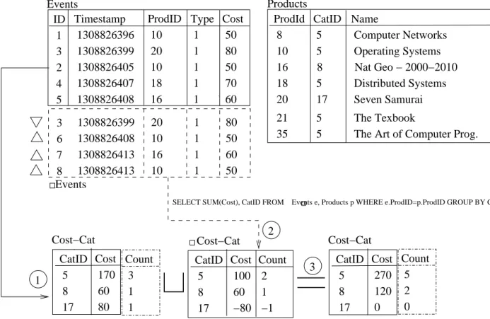
CHAPTER 4. MATERIALIZED VIEW MAINTENANCE—A THEORETICAL PERSPECTIVE21 Timestamp 1308826396 1308826399 1308826405 1308826407 1308826408 ProdID 10 20 10 18 16 Cost 50 80 50 70 60 Type 1 1 1 1 1 ID 1 3 2 4 5 Events ProdId 8 10 16 18 20 21 35 CatID 5 8 5 17 5 5 5 Name Computer Networks Nat Geo − 2000−2010 Distributed Systems Seven Samurai The Texbook

The Art of Computer Prog. Operating Systems Products 1308826399 1308826408 1308826413 1308826413 20 10 16 10 80 50 60 50 1 1 1 1 3 6 7 8 Cost 100 60 −80 Count 2 1 −1 CatID 5 8 17 Cost−Cat Cost 170 60 80 CatID 5 8 17 Cost−Cat Count 3 1 1 Events Count 5 2 0 Cost 270 120 0 CatID 5 8 17 Cost−Cat 1 2 3

SELECT SUM(Cost), CatID FROM Events e, Products p WHERE e.ProdID=p.ProdID GROUP BY CatID

Figure 4.1: Change Table Derivation after a Base Table Update

What remains to be computed are the rows to be inserted and deleted from the result of the SPJ query. Effectively, the database engine can apply the selection and join operators on a projection of the inserted and deleted rows from the base relation. The last follows from equation 4.2: σ(Bnew₁ ./B2) =σ(((Bold₁ −·OB1)]MB1)./B2)⇐⇒ σ(Bnew₁ ./B2) = (σ(Bnew1 ./B2)−·σ(OB1./B2))]σ(MB1./B2) =⇒ ( Mσ(Bold₁ ./B2) =MR=σ(MB1./B2) Oσ(Bold₁ ./B2) =OR=σ(OB1./B2) (4.2) Figure 4.1 illustrates the usage of the expressions provided in Equations 4.2 and 4.1. The example evaluates “SELECT SUM(Cost),CatIDFROMEvents e, Products pWHEREe.ProdID=p.ProdIDGROUP BYCatID” which is the total cost per category,

(29)

stored in theCost-Cat table, from theEvents fact table andProducts dimension table. The aggregation is performed in three phases discussed in the following paragraphs.

Initially, the Cost-Cat table has no entries. To compute the aggregation, the database engine has to inspect theEvents andProducts tables from scratch as shown in 1on Fig-ure 4.1. In addition to the attributes specified in the original query, the aggregate result table needs to maintain a counter for the SPJ rows grouped by the GROUP BY attributes. For example,ΠProdID,Cost,CatID(Events./ProdIDProducts)generates 3 results from category 5,

1 result from category 8, and 1 result from category 17.

After the initial aggregation has been computed, the database can readily maintain the aggregate result via change tables ( 2 on Figure 4.1). The second phase computes the change tableCost-Cat from theEvents insertions and deletions, prefixed with_Mand_O in the diagram. In the example shown on the diagram, there have been 3 insertions and one deletion. The change table is computed by joining the insertions and deletions with

Products and aggregating the result. The aggregation attributes and counts resulting from deletions have to be negated.

After the database engine has computed the aggregate result change table, it is ready to apply it to the result itself ( 2 on Figure 4.1). In order to complete the update, the database engine evaluates Cost-Cat ./ProdID Cost-Cat. Any change table rows which

are not present in the join result set have to be inserted into the aggregate view table. Otherwise, the matching attributes fromCost-Cat andCost-Catare simply summed and the corresponding aggregate view table row is updated or deleted if thecount attribute is0.

4.3.4 Change Table Propagation

Finally, change tables such as the one generated in the previous section can be readily propagated through relational operators using the equations listed on Table 4.1 [15]. The major relational operators used in data stores are Selection, Projection, Inner Join, Bag Union, andAggregation. Once a change table for an aggregation has been computed, it can be propagated and applied without reevaluating the whole aggregate expression.

Table 4.1: Change Propagation Equations [15]

Type V Vnew Refresh V

Selection σp(E1) σp(E1tU_ΘE1) VtU_θ σp(E1) σp(E1) Projection ΠA(E1) ΠA(E1tU_ΘE1) VtU_θ ΠA(E1) ΠA(E1) Inner Join E₁./JE2 (E1tU_ΘE1)./JE2 VtU_θ₁(E1./JE2) E1./J E2 Bag Union E₁]E₂ (E₁tU ΘE1)]E2 ((V−E2)t U θ E1)]E2 E1 Aggregation πG0_,_F(E₁) πG0_,_F(E₁tU ΘE1) Vt U3 θ3 πG0,F(E1) πG0,F(E1)

(30)

Chapter 5 System Design and API

This chapter discusses the implementation of the aggregate view maintenance techniques from Chapter 4. The main algorithm for automatically keeping aggregate views can be im-plemented either synchronously or asynchronously. The main difference between the two approaches is that in the former case, the base table update and change tableV computa-tion and applicacomputa-tion,E₁tU

ΘE1, are carried out in the same transaction while in the latter

case,V andE₁tU

ΘE1are deferred to a separate asynchronous transaction. Nevertheless,

in both cases the Cloud data store and its middleware need to support consistent read/write transactions.

Currently, CloudTPS is the only middleware providing strongly consistent transactions for web applications using non-relational data stores such as HBase and SimpleDB. The rest of this chapter provides details about the implementation of the synchronous and asyn-chronous view maintenance algorithms on CloudTPS.

5.1 Overview of CloudTPS

CloudTPS is a middleware for key-value data stores which provides strongly consistent and fault-tolerant transactions for web applications. The read-only transactions support look-ups by primary and secondary keys as well as equi-joins while the read/write trans-actions support insertion, deletion, and update transtrans-actions on individual rows. The read and write transactions are received by read/write and read-only transaction managers which distribute the work over a set of local transaction manager (LTM) nodes (Figure 5.1). Each LTM is responsible for handling a set of table rows identifiable by their primary keys. Both read and write transactions are submitted to the LTMs using the two phase commit protocol with the transaction manager serving as a coordinator. To ensure strong consistency, each transaction receives a global timestamp which is used for creating an execution order on the

(31)

CHAPTER 5. SYSTEM DESIGN AND API 24 Local Transaction Manager R/W Transaction Manager R/O Transaction Manager Worker

Cloud Data Store

Figure 5.1: CloudTPS Architecture

LTMs: transactions with newer timestamps than the timestamp of the current transaction are queued in FIFO order while all transactions with “old” timestamps are aborted.

To implement the synchronous and asynchronous change table view maintenance al-gorithms, the CloudTPS architecture needs to support more complex read/write operations consisting of transactions which execute an SPJ query plan and use the result as the input of update, insert, or delete sub-transactions. This modification is necessary in order to en-force consistency between the base relation updates and the maintained aggregate views. The modified read/write transaction mechanism is similar to the existing approach towards index table maintenance in CloudTPS and requires the implementation of a new transac-tion manager which uses the two phase commit protocol to coordinate the read and write sub-transactions. The next section discusses in detail the proposed CloudTPS modification.

5.2 Aggregate Queries for CloudTPS

The basic change table mechanism for CloudTPS is similar to the one pro-vided by Gupta et al and discussed in Chapter 4. For a given aggregate query

π_{f unc}₍_AggAttr₎_,_GB(σSelAtt(B1 ./JoinCond1 B2 ./JoinCond2 B3· · ·)), CloudTPS needs to

moni-tor the base relationsB1. . .Bnfor changes and re-evaluate the aggregate view upon update.

Algorithm 5.1 describes the synchronous version of this approach. Step 1 is executed once during the system’s initialization and it computes from scratch all aggregate views. After the initial step, all views can be incrementally updated from the old view and update values. Step 2 as shown on the diagram is executed as a single transaction and thus the performance of update queries is strongly dependent on the complexity of the materialized views in which the updated base relations participate: the heavier the aggregate expression is, the more intensivestep 2.ais.

(32)

CHAPTER 5. SYSTEM DESIGN AND API 25

Algorithm 5.1Basic Aggregate View Maintenance in CloudTPS .

1. Startup:ComputeV asπ_{f unc}(AggAttr),GB(σSelAtt(B1./JoinCond1 B2./JoinCond2 B3· · ·))

2. Coordinator LTM:Upon a base relation,B_k, update (a) ComputeB_k, defined as_MB_k]_OB_k

(b) Compute the aggregate change table, V as

π_{f unc}₍_AggAttr₎_,_GB_,_count(σSelAtt(B1 ./JoinCond1 B2 ./JoinCond2 B3· · ·Bk ./JoinCondk

...))

(c) ApplyV to V using the special join operator

The write performance upon base table updates can be generally improved by modify-ing the synchronous algorithm into Algorithm 5.2. The main difference between algorithms 5.1 and 5.2 is that the asynchronous version computes the aggregate view change table asynchronously and maintains additional CloudTPS tables storingB₁,B₂· · ·,B_n. The system initialization computes all aggregate views from scratch and clears the base relation change tables. Step 2 is executed as a transaction whenever a base table is updated and consists of updating the corresponding base relation change table B_k andB_k itself. The actual work performed by CloudTPS during write operations is significantly less than the workload in the synchronous algorithm as the change table computation which performs several join operations is postponed. The actual computation ofV andV’s application to the aggregate view table is performed in the last phase. InStep 3, the algorithm com-putesV from the base table change tables and the current value of the base tables. The asynchronous phase of the algorithm introduces a relatively heavy workload of O(n)join query plans.

5.3 Implementation

The CloudTPS architecture supports equi-join read-only queries and simple read/write transactions consisting of sub-transactions modifying at most one row. The two opera-tions are handled by a read-only and read/write transaction manager respectively. Even though this approach offers greater efficiency when handling the two query types, there is no mechanism allowing transactional execution of update operations using the input of read-only query plans. This problem can be addressed by either introducing table lock-ing preemptlock-ing concurrent same-table updates or a new transaction manager capable of handling the new read/write query. Unfortunately, despite its simplicity, the former ap-proach is prohibitively expensive as it sacrifices the read/write horizontal scalability by

(33)

Algorithm 5.2Asynchronous Aggregate View Maintenance in CloudTPS 1. Startup:

(a) ComputeV asπ_{f unc}(AggAttr),GB(σSelAtt(B1./JoinCond1 B2./JoinCond2 B3· · ·))

(b) ClearB₁,B₂· · ·,B_n

2. Coordinator LTM:Upon a base relation,B_k, update (a) ComputeB_k, defined as_MB_k]_OB_k

(b) CommitB_kas an ordinary CloudTPS table 3. Coordinator LTM:Asynchronous

(a) Retrieve base relations change tablesB1,B2· · ·,Bn

(b) Compute V = π_{f unc}(AggAttr),GB(σSelAtt(B1 ./JoinCond1 B2 ]B1 ./JoinCond1

B₂.−·B₁./JoinCond1 B2)

(c) ClearB₁,B₂· · ·,B_n

(d) ApplyV to V using the special join operator

decreasing the update transaction granularity. Thus the only viable solution is employing a mechanism capable of executing update transactions consuming the output of read-only operations. The rest of this section discusses the implementation of the new query manager handling transactions similar to the ones described in steps 2and3of algorithms 5.1 and 5.2.

5.3.1 Synchronous Computation

The synchronous version of the aggregate view maintenance algorithm maintains only one CloudTPS table representing the materialized aggregate view V. Both the view and base table change tables V and B₁. . .B_n are maintained in memory only during the up-date operations and do not require creating special CloudTPS tables. As the size of the change tables is relatively small due to the small-sized transactions characteristic for most web applications, these tables can be maintained on a single node serving as a transaction coordinator. Similarly to the read-only and read/write transaction managers, the aggregate view maintenance transaction manager uses a modified version of the two-phase commit protocol in order to guarantee consistency. Thus, when a node crashes, the only penalty incurred is restarting the computation. During the first phase of the protocol’s execution,

(34)

the coordinator node submits updates to the LTM participants. However, instead of send-ing only ACK and NACK messages, the LTMs return additional information resulting in adding more sub-transactions to the running transaction. The additional sub-transactions implement the logic in the view maintenance algorithm. If all the LTMs, including the ones which have been added later during the transaction’s course, send acknowledgments to the coordinator, the transaction is ready to be committed. The second phase commits all base table updates and the corresponding aggregate view table modifications.

The modified two phase commit protocol is shown of Figure 5.2. When a client-side application submits a read/write transaction modifying table A and C (not shown), the transaction manager executes the two phase commit protocol. The data item location and the transaction management mechanism is similar to the one present in the unmodified CloudTPS transaction manager:

1. In order to ensure consistency, each transaction is assigned a global timestamp which is used for queuing conflicting transactions in FIFO order. Transactions with “stale” timestamps are aborted;

2. The coordinator identifies all LTMs responsible for each sub-transaction and builds all relevant sub-transaction groups to be submitted;

3. Each LTM votes whether its sub-transactions can be committed.

However, instead of simply committing the base table updates upon consensus among the LTMs, the coordinator needs to compute sequentially the base table’s change tables, the aggregate view change table (V), and the updated view after the application of V. As the change tables can easily fit into a single node’s main memory, the coordinator proceeds with the join algorithm used in the read-only transaction manager to compute

σAttributesB1./B2. . .Bn. Finally, afterV =πAgg,Func,_countσAttributesB1./B2. . .Bnhas

been computed, the algorithm proceeds by adding to the current transaction more read-write sub-transaction in order to applyV. Upon failure, the coordinator aborts the trans-action and consequently, the CloudTPS tables remain consistent as neither the base table modifications nor the aggregate view is committed.

The approach described in the previous paragraphs is shown on Figure 5.2. As shown on the diagram, A and B are base tables which participate in the join query

σID,Cost,Prod,CatA ./Prod B defined by some client application. At a certain point during

its execution, the web-application submits to LT M₃ a read/write transactions modifying tables A and C (not shown). LT M₃ serves as the transaction’s coordinator and needs to computeA,V, and apply the change table toV. The transaction is executed as follows: 1. LT M₃starts the two-phase commit protocol and submits the base table updates to the responsible LTMs (LT M₁,LT M₂,LT M₄) 1. For simplicity, the CloudTPS secondary key index maintenance mechanism has been omitted from the diagram;

(35)

CHAPTER 5. SYSTEM DESIGN AND API 28 LTM 1 LTM 2 LTM 3 LTM 4 1

{

A(R3, R4, R5) C(R5) 1

Add A(R4), A(R5) 1 2 A ID Cost 2 3 1 10 10 50 1 1 8 Prod T 1 T 2 B Cat 1 20 25 8 Prod A 4 5 3 10 20 50 1 1 8 V ID Cost 2 3 1 10 10 50 1 1 8 Prod Cat 20 20 25 LTM 5 3 Add A(R3) 3

1 Submit base table updates 2 Compute Base Change Table 3 Compute View Change Table 4 Apply View Change Table

V = 4 5 3 10 20 50 1 1 8 20 20 25 A B LTM 6 4 5 Commit 5 5 5 5 Update Transaction Add none Submit A(R4,R5) R/O Vote Submit V(3,4,5) Add none Submit A(R3)

Figure 5.2: Synchronous Computation Two-Phase Commit Protocol

2. LT M1,LT M2, andLT M4piggyback on theirACK messages all the attributes

associ-ated with the base table being updassoci-ated so that the coordinator can computeA 2. This step is necessary because a read/write transaction should not necessarily contain all the attributes of the rows to be updated. After all votes have been received, the coordinator has the values of all attributes of rows 3,4, and 5 and can proceed to the next step;

3. The coordinator, LT M3, submits read-only sub-transactions to LT M5 to compute σID,Cost,Prod,CatA./ProdB3. For simplicity, the CloudTPS secondary key queries

have been omitted from the diagram. The query mechanism is the same as the one employed by the read-only transaction manager. The coordinator submits the query to the LTMs responsible for the data items and if necessary new read-only look-ups are added if secondary keys are used. After all votes have been received, the coordi-nator computesV =πCost,_countσID,Cost,Prod,CatA./ProdBand is ready to submit

the final read/write sub-transactions in order to update the aggregate view table; 4. The aggregate view maintenance operatortU_Θ is implemented as a special write

op-eration similar to insertion, deletion, and update and will be described in detail in Section5.3.2. AfterV has been computed in the previous step, the coordinator is ready to update the aggregate view asVtU_ΘV 4. In the specific example,LT M₃

(36)

5. After all involved LTMs have submitted their votes to the coordinator LT M₃, the transaction can be either committed or aborted.

5.3.2 CloudTPS Aggregate View Refresh Operator

As discussed in Section 4.3.2, the aggregate view refresh operator applies the aggregate view change tableV to the aggregate viewV in order to reflect any base table changes. To this end, both the aggregate view and its change table need to maintain an additional attribute, _count, which keeps track of the number of rows aggregated by theGROUP BY

statement. When applying the change table to the view itself, the refresh operator applies the specified aggregate function with positive change table aggregate attributes for inser-tions and negative values for deleinser-tions. If _count =0 for some row in the aggregate view, the row has to be deleted. Otherwise, the row needs to be either updated if it previously existed in the view or inserted.

Matching rows from the aggregate viewV with rows from its change tableV is equiv-alent to an equi-join operation on theGROUP BY attributes. Moreover, the operation can be sped-up by introducing a primary key consisting of the concatenation of theGROUP BY

attributes so that any secondary key look-ups and index table are eliminated. Thus,V and the correspondingV need to have two additional attributes used internally by CloudTPS:

_groupBy(primary key) and_count(count of aggregated rows). The refresh operator can be readily implemented using the two-phase commit protocol as shown in Algorithm 5.3.

5.3.3 Asynchronous Computation

As discussed in the beginning of this chapter, despite being strongly consistent, the syn-chronous aggregate view maintenance approach introduces relatively heavy workloads and can become expensive with larger read/write transactions. The main reason behind this performance issue is the large number of sub-transactions the coordinator needs to add in order to complete the a read/write operation on an aggregate base table. The asynchronous version of the computation shown in Algorithm 5.2 offers greater flexibility at the expense of allowing staleness in the aggregate views.

In the asynchronous version of the aggregation computation, CloudTPS needs to main-tain base table change tables which are used for the deferred derivation of the aggregate view. Just like in the synchronous algorithm, the coordinator node identifies the LTMs re-sponsible for the data items to be updated and waits for receiving the complete rows after submitting the sub-transactions. However, after receiving the LTM votes, instead of pro-ceeding with computingV, the coordinator adds sub-transactions updating the base table change tables and waits for the final votes before committing. This approach decreases considerably the number of sub-transactions submitted by the coordinator node and allows for an asynchronous view update as it preserves enough information to computeV.

(37)

Algorithm 5.3Aggregate View Table Refresh

1. The coordinator generates and submits arefresh sub-transaction from eachV row and uses the primary key to identify the LTM handling potential view table matches. 2. Each LTM performs one of the following:

(a) Inserts a row if there is no match on the_groupByattribute

(b) Carries out the aggregate operations if there is a match on the _groupBy at-tribute and does one of the following:

i. Deletes the row if _countnew=0 ii. Performs an update if _countnew6=0 3. Upon LTM consensus the transaction is committed

The second phase of the asynchronous algorithm obtains and applies V using

B₁. . .B_n. As in the synchronous algorithm, a random node is selected for a transaction coor-dinator which computes V =π_{f unc}₍_AggAttr₎_,_GB(σSelAtt(B1./JoinCond1 B2]B1./JoinCond1

B2.−·B1./JoinCond1 B2). The previous expression has a simple query plan which can

be readily handled by the logic of the read-only transaction manager. After the computa-tion, tablesB₁. . .B_nare cleared and the aggregate view change table is applied as described in Section 5.3.2.

5.4 Aggregate View Maintenance API

The aggregate view maintenance programming interface closely resembles the CloudTPS read-only query plan API. All aggregate queries need to be statically registered in advance so that the initial aggregate views can be computed during the system’s initialization. An aggregate query can be defined as a collection of “JoinTable” and “JoinEdge” objects which have the same semantics as defined by Zhou at al. The only difference between declaring a standard select-project-join query plan and aggregate query plan is the additional definition ofGROUP BY columns and aggregate functions.

(38)

Chapter 6 Evaluation

This section provides an experimental evaluation of the synchronous and asynchronous aggregate view maintenance algorithms presented in Chapter 5. The modified CloudTPS architecture was executed on top of HBase running on the DAS-3 computer cluster which comprises 85 nodes running Linux on dual core 2.4 GHz CPUs and using 4 GB memory. Each node used in the experiments functioned either as an LTM or load generator. The LTM role is described in detail in Chapter 5 while the load generator submits update transactions introducing controlled workloads to the CloudTPS framework.

The aggregate view maintenance aggregate algorithm was evaluated both in term of micro-benchmarks covering specific implementation details and the standard TPC-W benchmark providing a typical workload for an e-commerce web application.

6.1 Experimental Setup

Figure 6.1 shows the experimental setup for the aggregate view maintenance synchronous and asynchronous algorithms. For each evaluation run, a subset of the DAS-3 nodes was assigned either aload generatororlocal transaction managerrole. Each load generator is a single-threaded application generating update transactions modifying a specified number of data items in CloudTPS-managed tables in the Cloud data store.

None of the load generators submits read-only query plans as evaluating an aggregate query consists of a simple look-up in the aggregate view table. Thus both the micro-benchmarks and TPC-W application simply populate their CloudTPS tables and subse-quently send updates. As the LTMs are interconnected via a Gigabit LAN, any network latency effects can be ignored. As the view maintenance table update implementation is based on the CloudTPS secondary key index maintenance, based on the two phase commit protocol, fault tolerance and network partitioning has been largely untested as these topics are covered in detail in [23].

Aggregate Queries in NoSQL Cloud Data Stores