WIND TURBINES WITH ASYNCHRONOUS
ELECTRICAL GENERATORS
He gave the wind its weight. Job 28:25.
In the last chapter we discussed some of the features of wind turbines synchronized with the electrical grid. There are a number of advantages to synchronized operation in that frequency and voltage are controlled by the utility, reactive power for induction generators is available, starting power for Darrieus turbines is available, and storage requirements are minimal. These advantages would indicate that most of the wind generated electricity in the United States will be produced in synchronism with the utility grid.
Historically, however, most wind electric generators have been attached to asynchronous loads. The most common load, especially before about 1950, has been a bank of batteries which in turn supply power to household appliances. Other loads include remote communication equipment, cathodic protection for buried pipelines, and direct space heating or domestic hot water heating applications. These wind electric generators have been small in size, usually less than 5 kW, and have usually been located where utility power has not been available.
We can expect the use of asynchronous electricity to continue, and perhaps even to grow, for a number of reasons. The use of wind power at remote communication sites for charging batteries can be expected to increase as less expensive, more reliable wind turbines are devel-oped. Space heating and domestic hot water heating are natural applications where propane or oil are now being used. Existing fossil fueled equipment can be used as backup for the wind generated energy. Another large potential market would be the many thousands of villages around the world which are not intertied with any large utility grid. Economics may preclude the possibility of such a grid, so each village may be forced to have its own electric system if it is to have any electricity at all. An asynchronous system which could operate a community refrigerator for storing medicine, supply some light in the evening, and provide power for cooking meals (to help prevent deforestation) would be a valuable asset in many parts of the world.
One final reason for having asynchronous capability on wind turbines in the United States would be the possibility of its being needed if the electrical grid should fall apart. If any of the primary sources of oil, coal, and nuclear energy should become unavailable for any reason, there is a high probability of rotating blackouts and disassociation of the grid. Wind turbines may be able to provide power to essential applications during such periods if they are properly equipped. Such wind turbines will have to be capable of being started without utility power, and will also require some ability to maintain voltage and frequency within acceptable limits. The three most obvious methods of providing asynchronous electricity are the dc generator, the ac generator, and the self- excited induction generator. Each of these will be discussed in this chapter. Various loads will also be discussed. The number of combinations of generators
and loads is almost limitless, so only a few combinations will be considered in any detail.
1 ASYNCHRONOUS SYSTEMS
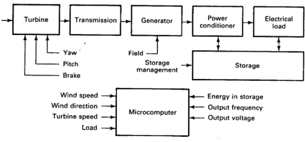
In the previous two chapters, we examined combinations of wind turbines, transmissions, and generators connected to the electrical grid. The electrical grid was assumed to be able to accept all the power that could be generated from the wind. The grid was also able to maintain voltage and frequency, and was able to supply any reactive power that was needed. When we disconnect ourselves from the grid, these advantages disappear and we must compensate by adding additional equipment. The wind system design will be different from the synchronous system and will contain additional features. A possible system block diagram is shown in Fig. 1.
Figure 1: Block diagram of asynchronous electrical system.
In this system, the microcomputer accepts inputs such as wind speed and direction, turbine speed, load requirements, amount of energy in storage, and the voltage and frequency being delivered to the load. The microcomputer sends signals to the turbine to establish proper yaw (direction control) and blade pitch, and to set the brakes in high winds. It sends signals to the generator to change the output voltage, if the generator has a separate field. It may turn off non critical loads in times of light winds and it may turn on optional loads in strong winds. It may adjust the power conditioner to change the load voltage and frequency. It may also adjust the storage system to optimize its performance.
It should be mentioned that many wind electric systems have been built which have worked well without a microcomputer. Yaw was controlled by a tail, the blade pitch was fixed, and the brake was set by hand. The state of charge of the storage batteries would be checked once or twice a day and certain loads would be either used or not used depending on the wind and the state of charge. Such systems have the advantages of simplicity, reliability, and minimum cost,
with the disadvantages of regularly requiring human attention and the elimination of more nearly optimum controls which demand a microcomputer to function. The microcomputer and the necessary sensors tend to have a fixed cost regardless of the size of turbine. This cost may equal the cost of a 3-kW turbine and generator, but may only be ten percent of the cost of a 100 kW system. This makes the microcomputer easier to justify for the larger wind turbines.
The asynchronous system has one rather interesting mode of operation that electric utilities do not have. The turbine speed can be controlled by the load rather than by adjusting the turbine. Electric utilities do have some load management capability, but most of their load is not controllable by the utilities. The utilities therefore adjust the prime mover input (by a valve in a steam line, for example) to follow the variation in load. That is, supply follows demand. In the case of wind turbines, the turbine input power is just the power in the wind and is not subject to control. Turbine speed still needs to be controlled for optimum performance, and this can be accomplished by an electrical load with the proper characteristics, as we shall see. A microcomputer is not essential to this mode of operation, but does allow more flexibility in the choice of load. We can have a system where demand follows supply, an inherently desirable situation.
As mentioned earlier, the variety of equipment in an asynchronous system is almost lim-itless. Several possibilities are shown in Table 6.1. The generator may be either ac or dc. A power conditioner may be required to convert the generator output into another form, such as an inverter which produces 60 Hz power from dc. The electrical load may be a battery, a resistance heater, a pump, a household appliance, or even exotic devices like electrolysis or fertilizer cells.
Not every system requires a power conditioner. For example, a dc generator with battery storage may not need a power conditioner if all the desired loads can be operated on dc. It was not uncommon for all household appliances to be 32 V dc or 110 V dc in the 1930s when small asynchronous wind electric systems were common. Such appliances disappeared with the advent of the electrical grid but started reappearing in recreational vehicles in the 1970s, with a 12-V rating. There are no serious technical problems with equipping a house entirely with dc appliances, but costs tend to be higher because of the small demand for such appliances compared with that for conventional ac appliances. An inverter can be used to invert the dc battery voltage to ac if desired.
TABLE 6.1 Some equipment used in asynchronous systems
• ELECTRICAL GENERATOR – DC shunt generator
– Permanent-magnet ac generator – AC generator
– Field modulated generator – Roesel generator
• POWER CONDITIONER – Diode rectifier
– Inverter
– Solid-state switching system
• ELECTRICAL LOAD – Battery
– Water heater – Space (air) heater – Heat pump – Water pump – Fan – Lights – Appliances – Electrolysis cells – Fertilizer cells
If our generator produces ac, then a rectifier may be required to deliver the dc needed by some loads or storage systems. Necessary switching may be accomplished by electromechanical switches or by solid state switches, either silicon controlled rectifiers (SCRs) or triacs. These switches may be used to match the load to the optimum turbine output.
The electrical load and storage components may have items which operate either on ac or dc, such as heating elements, on ac only, such as induction motors, lights, and most appliances, or dc only, such as electrolysis cells and batteries. Some of the devices are very long lived and inexpensive, such as heating elements, and others are shorter lived and more expensive, such as batteries and electrolysis cells. Some items can be operated in almost any size. Others, such as electrolysis cells and fertilizer cells, are only feasible in rather large sizes.
Economics must be carefully considered in any asynchronous system. First, a given task must be performed at an acceptable price. Second, as many combinations as possible should be examined to make sure the least expensive combination has been selected. And third, the alternatives should be examined. That is, a wind turbine delivers either rotational mechanical power or electrical power to a load, both of which are high forms of energy, and inherently expensive. If it is desired to heat domestic hot water to 40oC, a flat plate solar collector would normally be the preferred choice since only low grade heat is required. If the wind turbine
were driving a heat pump or charging batteries as a primary function, then heating domestic hot water with surplus wind power might make economic sense. The basic rule is to not go to any higher form of work than is necessary to do the job. Fixed frequency and fixed voltage systems represent a higher form of work than variable frequency, variable voltage systems, so the actual needs of the load need to be examined to determine just how sophisticated the system really needs to be. If a simpler system will accomplish the task at less cost, it should be used.
2 DC SHUNT GENERATOR WITH BATTERY LOAD
Most people immediately think of a simple dc generator and a battery storage system when small wind turbines are mentioned. Many such systems were placed in service in the 1930s or even earlier. They provided power for a radio and a light bulb or two, and occasionally power for some electrical appliances. Some of the machines, especially the Jacobs, seemed almost indestructible. A number of these machines have provided service for over fifty years. These machines nearly all disappeared between 1940 and 1950, partly because centrally gen-erated electricity was cheaper and more reliable, and partly because some Rural Electrical Cooperatives (REC) would not supply electricity to a farm with an operating wind electric system.
Today, such small dc systems still have very marginal economics when centrally generated electricity is available. Their primary role would then seem to be to supply limited amounts of power to isolated loads such as weather data stations, fire lookout towers, and summer cottages. They may also provide a backup or emergency system which can be used when centrally generated power is not available due to equipment failure or fuel shortages.
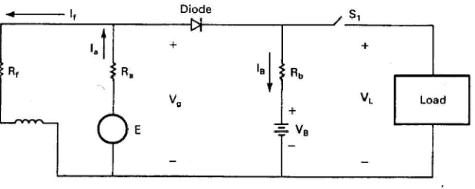
A diagram of a simple dc shunt generator connected to a battery is shown in Fig. 2. This circuit has been widely used since copper oxide and selenium rectifiers (diodes) were developed in the 1930s. Silicon diodes with much superior characteristics were developed in the 1950s and are almost exclusively used today. The diode allows current to flow from the generator to the battery, but prevents current flow in the opposite direction. This prevents the battery from being discharged through the generator when the generator voltage is below the battery voltage.
The generator consists of a rotor orarmature with resistance Raand a field winding with
resistanceRf on the stator. The armature currentIais brought out of the machine by brushes
which press against thecommutator, a set of electrical contacts at one end of the armature. The generator terminal voltage Vg causes a field currentIf to flow in the field winding. This
field current flowing in a coil of wire, indicated by an inductor symbol on the left side of Fig. 2, will produce a magnetic flux. The interaction of this flux and the rotating conductors in the armature produces the generated electromotive force (emf)E, which is given by
Figure 2: DC shunt generator in a battery-charging circuit.
E =ksωmΦp V (1)
where Φp is the magnetic flux per pole, ωm is the mechanical angular velocity of the rotor,
and ks is a constant involving the number of poles and number of turns of conductors. We
see that the voltage increases with speed for a given flux. This means that at low speeds the generated emf will be less than the battery voltage. This has the advantage that the turbine will not be loaded at low rotational speeds, and hence will be easier to start.
The generator rotational speedncan be determined from the angular velocity ωm by
n= 60ωm
2π r/min (2)
The induced voltageEis in series with the resistanceRaof the rotor or armature windings.
In this simple model,Ra would also include the resistance of the brushes on the commutator
bars.
The current flowIf (theexcitation current) in the field winding around the poles is given
by
If = V g
Rf
A (3)
The field winding has inductance, but the reactanceωLis zero because only dc is involved. Therefore only the resistances are needed to compute currents or voltages.
The flux does not vary linearly with field current because of the saturation of the magnetic circuit. The flux will increase rapidly with increasingIf for small values ofIf, but will increase
more slowly asIf gets large and the iron of the machine gets more saturated. Also, the flux is
not exactly zero whenIf is zero, due to the residual magnetism of the poles. The iron tends
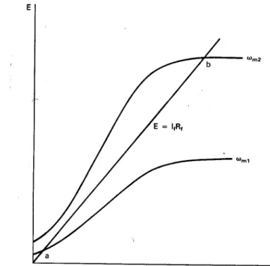
generated emfEwill be greater than zero whenever the armature is spinning, even though the field current is negligible. These effects of the iron circuit yield a plot ofE versusIf such as
shown in Fig. 3. E starts at a positive value, increases rapidly for small If, and finally levels
off for larger If. Two angular velocities, ωm1 and ωm2, are shown on the figure. Increasing
ωm merely expands the curve for E without changing its basic shape.
Figure 3: Magnetization curve of dc generator. The generated emf E is given by Kirchhoff’s voltage law as
E =IaRa+IfRf V (4)
Rais much smaller thanRf, so when the diode current is zero, which causesIa=If, theIaRa
term is very small compared withRfIf. Therefore, to a first approximation, we can write
E IfRf (5)
This equation is just a straight line passing through the origin of Fig. 3. We therefore have a voltage E being constrained by both a nonlinear dc generator and a linear resistor. The generator requires the voltage to vary along the nonlinear curve while the field resistor requires it to vary along the straight line. Both requirements are met at the intersection of the nonlinear curve and the straight line, and this intersection defines the equilibrium oroperating
point. When the generator is turning at the angular velocity ωm1, voltage and current will
build up only to point a. This is well below the capability of the generator and is not a desirable operating point. If the angular velocity is increased toωm2 the voltage will build up
to the value at point b. This is just past the knee of the magnetization curve and is a good operating point in that small changes in speed or field resistance will not cause large changes inE.
Another way of changing the operating point is to change the field resistance Rf. The
slope of the straight line decreases as Rf decreases so the operating point can be set any
place along the magnetization curve by the proper choice of Rf. There are some practical
limitations to decreasingRf, of course. Rf usually consists of an external variable resistance
plus the internal resistance of a coil of many turns of fine wire. Therefore Rf can not be
reduced below the internal coil resistance.
The mode of operation of this generator is referred to as a self-excited mode. The residual magnetism of the generator produces a small flux, which causes a small voltage to appear across the field winding when the generator rotor is rotated. This small voltage produces a small field current which helps to boost E to a larger value. This larger E produces a still larger field current, which produces a still larger E, until equilibrium is reached. The equilibrium point will be at small values ofE for low speeds or high field resistance, and will increase rapidly to a point past the knee of the magnetization curve as speed or field resistance reaches some critical value. Once the voltage has built up to a value close to the rated voltage, the generator can supply current to a load.
We now want to examine the operation of the self-excited shunt generator as a battery charger, with the circuit of Fig. 2. We assume that switch S1 is open, that the diode is an open circuit whenE is less than the battery voltage VB and a short circuit when E is greater
thanVB, and thatRB includes the resistance of the diode and connecting wires as well as the
internal resistance of the battery. When the diode is conducting, the relationship betweenE
andVB is
E=VB+IfRa+IB(Ra+Rb) V (6)
The term IfRa is a very small voltage and can be neglected without a serious loss of
accuracy. If we do so, the battery current is given by
IB E−VB
Ra+Rb
A (7)
The electrical power produced by the shunt generator when the diode is conducting is given by
Pe =EIaEIf +E
(E−VB
Ra+Rb
The electrical power delivered to the battery is
PB =VBIB W (9)
The electrical power can be computed as a function of angular velocity if all the quantities in Eq. 8 are known. In practice, none of these are known very precisely. Etends to be reduced below the value predicted by Eq. 1 by a phenomenon called armature reaction. The resistance of the copper wire in the circuit increases with temperature. Ra and Rb include the voltage
drops across the brushes of the generator and the diode, which are quite nonlinear. And finally, VB varies with the state of charge of the battery. Each system needs to be carefully
measured if a detailed curve of power versus rotational speed is desired. General results or curves applicable to a wide range of systems are very difficult to obtain, if not impossible.
Example
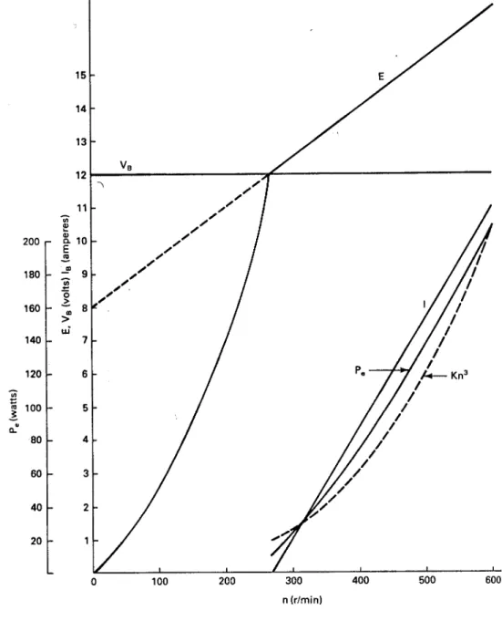
The Wincharger Model 1222 is a 12-V, 15-A self-excited dc shunt generator used for charging 12-V batteries. By various crude measurements and intelligent estimates, you decide thatRf = 15 Ω,Ra = 0.2 Ω,Rb = 0.25 Ω,VB = 12 V, andE = 0.015n+ 8 V. This expression forE includes the armature reaction over the normal operating range, hence is much flatter than the ideal expression of Eq. 1. Assume the diode is ideal (no forward voltage drop when conducting) and plot E, IB, and Pe for n between 0 and 600 r/min.
We first observe that IB = 0 wheneverE≤VB. The rotational speed at which the battery starts to charge is found by settingE=VB and solving forn.
0.015n+ 8 = 12
n= 4
0.015 = 270 r/min
The battery current will vary linearly with E and therefore with the rotational speed, according to Eq. 7. We can plot the currentIB by just finding one more point and drawing a straight line. Atn = 600 r/min, the battery current is given by
IB 0.015(600) + 80 −12
.2 + 0.25 = 11 A
The electrical power generated is nonlinear and has to be determined at several rotational speeds to be properly plotted. When this is done, the desired quantities can be plotted as shown in Fig. 4. The actual generatedEstarts at zero and increases as approximately the square of the rotational speed until diode current starts to flow. Both flux and angular velocity are increasing, so Eq. 1 would predict such a curve. When the diode current starts to flow, armature reaction reduces the rate of increase of
E. The flux also levels off because of saturation. E can then be approximated for speeds above 270 r/min by the straight line shown, which could then be extrapolated backward to intersect the vertical axis, at 8 V in this case.
The current will also increase linearly, giving a square law variation in the electrical power. The optimum variation of power would be a cubic function of rotational speed, which is shown as a dashed curve in Fig. 4. The discontinuity in E causes the actual power variation to approximate the ideal rather closely, which would indicate that the Wincharger is reasonably well designed to do its job.
Figure 4: Variation ofE, IB, andPe for Wincharger 1222 connected to a 12-V battery.
One other aspect of operating shunt generators needs to be mentioned. When a new generator is placed into service, it is possible that there is no net residual magnetism to cause a voltage buildup, or that the residual magnetism is oriented in the wrong direction. A short
application of rated dc voltage to the generator terminals will usually establish the proper residual magnetism. This should be applied while the generator is stopped, so current will be well above rated, and should be applied for only a few seconds at most. Only the field winding needs to experience this voltage, so if the brushes can be lifted from the commutator, both the generator and the dc supply will experience much less shock.
3 PERMANENT MAGNET GENERATORS
A permanent magnet generator is like the synchronous or ac generator discussed in the previ-ous chapter except that the rotor field is produced by permanent magnets rather than current in a coil of wire. This means that no field supply is needed, which reduces costs. It also means that there is noI2R power loss in the field, which helps to increase the efficiency. One disadvantage is that the reactive power flow can not be controlled if the PM generator is connected to the utility network. This is of little concern in an asynchronous mode, of course. The magnets can be cast in a cylindrical aluminum rotor, which is substantially less expen-sive and more rugged than the wound rotor of the conventional generator. No commutator is required, so the PM generator will also be less expensive than the dc generator of the previous section. These advantages make the PM generator of significant interest to designers of small asynchronous wind turbines.
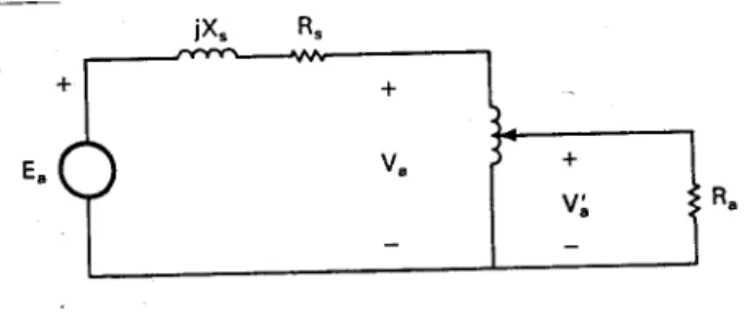
One load which might be used on a PM generator would be a resistance heating system for either space or hot water. Such a system is shown in Fig. 5. The three line-to-neutral generated voltagesEa,Eb, andEc are all displaced from each other by 120 electrical degrees.
The line-to-neutral terminal voltages are also displaced from each other by 120o if the three-phase load is balanced (Ra =Rb =Rc). The current Ia is given by
Ia= Ea
Rs+jXs+Ra
= Va
Ra
A (10)
whereXs is the synchronous reactance,Rs is the winding resistance, andRa is the resistance
of one leg or one phase of the load resistance.
The neutral currentIn is given by the sum of the other currents.
In=Ia+Ib+Ic A (11)
If the load is balanced, then the neutral current will be zero. In such circumstances, the wire connecting the neutrals of the generator and load could be removed without affecting any of the circuit voltages or currents. The asynchronous system will need the neutral wire connected, however, because it allows the single-phase voltages Va, Vb, andVc to be used for
other loads in an unbalanced system. Several single-phase room heaters could be operated independently, for example, if the neutral wire is in place.
Figure 5: Permanent-magnet generator connected to a resistive load.
It is desirable to maintain the three line currents at about the same value to minimize torque fluctuations. It is shown in electrical machinery texts that a three-phase generator will have a constant shaft torque when operated under balanced conditions. A single-phase generator or an unbalanced three-phase generator has a torque that oscillates at twice the electrical frequency. This makes the generator noisy and tends to shorten the life of the shaft, bearings, and couplers. This is one of the primary reasons single-phase motors and generators are seldom seen in sizes above about 5 kW. The PM generator will have to be built strongly enough to accept the turbine torque fluctuations, so some imbalance on the generator currents should not be too harmful to the system, but the imbalance will need to be minimized to keep the noise level down, if for no other reason.
The electrical output powerPe (the power delivered to the load) of the PM generator per
phase is
Pe=Ia2Ra W/phase (12)
The magnitude of the current is
|Ia|= |Ea|
(Rs+Ra)2+Xs2
A (13)
Therefore the output power can be expressed as
Pe = E
2
aRa
(Rs+Ra)2+Xs2
W/phase (14)
The generated voltageEa can be written as
Ea=keω V (15)
This is basically the same equation as Eq. 1. Here the constant ke includes the flux per
between the mechanical angular velocityωmand the electrical angular velocity ω. A four pole
generator spinning at 1800 r/min will haveωm= 188.5 rad/s andω= 377 rad/s, for example.
The ratio of electrical to mechanical angular velocity will be 1 for a two pole generator, 2 for a four pole, 3 for a six pole, and so on.
This variation in generated voltage with angular velocity means that a PM generator which has an open-circuit rms voltage of 250 V line to line at 60 Hz when the generator rotor is turning at 1800 r/min will have an open circuit voltage of 125 V at 30 Hz when the generator rotor is turning at 900 r/min. Wide fluctuations of voltage and frequency will be obtained from the PM generator if the wind turbine does not have a rather sophisticated speed control system. The PM generator must therefore be connected to loads which can accept such voltage and frequency variations.
Lighting circuits would normally not be appropriate loads. Incandescent bulbs are not bright enough at voltages 20 percent less than rated, and burn out quickly when the voltages are 10 percent above rated. There will also be an objectionable flicker when the frequency drops significantly below 60 Hz. Fluorescent bulbs may operate over a slightly wider voltage and frequency range depending on the type of bulb and ballast. If lighting circuits must be supplied by the PM generator, consideration should be given to using a rectifier and battery system just for the lights.
It should be noticed that the rating of the PM generator is directly proportional to the rotational speed. The rated current is related to the winding conductor size, which is fixed for a given generator, so the output power VaIa will vary as Ea or as the rotational speed.
The resistance Ra has to be varied as Ea varies to maintain a constant current, of course.
This means that a generator rated at 5 kW at 1800 r/min would be rated at 10 kW at 3600 r/min because the voltage has doubled for the same current, thus doubling the power. The limitations to this increase in rating are the mechanical limitations of rotor and bearings, and the electrical limitations of the insulation.
In Chapter 4 we saw that the shaft power input to the generator needs to vary as n3 for the turbine to operate at its peak efficiency over a range of wind speeds and turbine speeds. Since n and ω are directly proportional, and the efficiency is high, we can argue that the output power of the PM generator should vary asω3 for the generator to be an optimum load for the turbine. The actual variation can be determined by explicitly showing the frequency dependency of the terms in Eq. 14. In addition to Ea, there is the reactance Xs, which is
given by
Xs =ωLs Ω (16)
The termLs is the inductance of the generator windings. It is not a true constant because of
saturation effects in the iron of the generator, but we shall ignore that fact in this elementary treatment.
Pe= k
2
eω2Ra
(Rs+Ra)2+ω2L2s
W/phase (17)
We see that at very low frequencies or for a very large load resistance thatPe increases as the
square of the frequency. At very high frequencies, however, whenωLs is larger thanRs+Ra,
the output power will be nearly constant as frequency increases. At rated speed and rated power, Xs will be similar in magnitude to Rs+Ra and the variation of Pe will be nearly
proportional to the frequency.
We therefore see that a PM generator with a fixed resistive load is not an optimum load for a wind turbine. If we insist on using such a system, it appears that we must use some sort of blade pitching mechanism on the turbine. The blade pitching mechanism is a technically good solution, but rather expensive. The costs of this system probably far surpass the cost savings of the PM generator over other types of generators.
One alternative to a fixed resistance load is a variable resistance load. One way of varying the load resistance seen by the generator is to insert a variable autotransformer between the generator and the load resistors. The circuit for one phase of such a connection is shown in Fig. 6. The basic equations for an autotransformer were given in the previous chapter. The voltage seen by the load can be varied from zero to some value above the generator voltage in this system. The power can therefore be adjusted from zero to rated in a smooth fashion. A microcomputer is required to sense the wind speed, the turbine speed, and perhaps the rate of change of turbine speed. It would then signal the electrical actuator on the autotransformer to change the setting as necessary to properly load the turbine. A good control system could anticipate changes in turbine power from changes in wind speed and keep the load near the optimum value over a wide range of wind speeds.
Figure 6: Load adjustment with a variable autotransformer.
One problem with this concept is that the motor driven three-phase variable autotrans-former probably costs as much as the PM generator. Another problem would be mechanical reliability of the autotransformer sliding contacts. These would certainly require regular main-tenance. We see that the advantages of the PM generator in the areas of cost and reliability have been lost in using a variable autotransformer to control the load.
Another way of controlling the load, which eliminates the variable autotransformer, is to use a microcomputer to switch in additional resistors as the wind speed and turbine speed
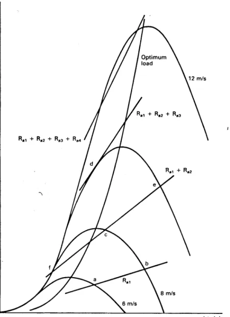
increase. The basic circuit is shown in Fig. 7. The switches can be solid state (triacs) which are easily controlled by microcomputer logic levels and which can withstand millions of operating cycles. Costs and reliability of this load control system are within acceptable limits. Unfortunately, this concept leads to a marginally unstable system for the Darrieus turbine and possibly for the horizontal axis propeller turbine as well. The instability can be observed by examining the electrical power output of the Sandia 17 m Darrieus as shown in Fig. 8. The power output to an optimum load is seen to pass through the peak turbine power output for any wind speed, as was discussed in Chapter 4. The load powers for the four different resistor combinations are shown as linear functions of n around the operating points. These curves are reasonable approximations for the actualPe curves, as was pointed out by the discussion
following Eq. 17. We do not need better or more precise curves forPe because the instability
will be present for any load that varies at a rate less thann3.
Figure 7: Load adjustment by switching resistors.
We assume that the load power is determined by the curve markedRa1 and that the wind
speed is 6 m/s. The turbine will be operating at point a. If the wind speed increases to 8 m/s, the turbine torque exceeds the load torque and the turbine accelerates toward pointb. If the second resistor is switched in, the load power will increase, causing the turbine to slow down. The new operating point would then be point c. If the wind speed drops back to 6 m/s, the load power will exceed the available power from the turbine so the turbine has to decelerate. If the load is not removed quickly enough, the operating point will pass through point f and the turbine will stall aerodynamically. It could even stop completely and need to be restarted. The additional load must be dropped as soon as the turbine starts to slow down if this condition is to be prevented.
Another way of expressing the difficulty with this control system is to note that the speed variation is excessive. Suppose the resistance is Ra1+Ra2 +Ra3 and we have had a steady
wind just over 10 m/s. If the wind speed would slowly decrease to 10 m/s, the turbine would go to the operating point marked d, and then as it slowed down further, the load would be switched toRa1+Ra2. The turbine would then accelerate to pointe. The speed would change
from approximately 50 to 85 r/min for this example. This is a very large speed variation and may pose mechanical difficulties to the turbine. It also places the operating point well down from the peak of the power curve, which violates one of the original reasons for considering an asynchronous system, that of maintaining peak power over a range of wind speeds and turbine rotational speeds. We therefore see that the PM generator with a switched or variable resistive
Figure 8: Electrical power output of Sandia 17-m Darrieus in variable-speed operation. load is really not a very effective wind turbine load. The problems that are introduced by this system can be solved, but the solution will probably be more expensive than another type of system.
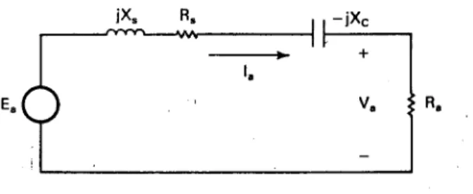
Another alternative for matching the load power to the turbine power is a series resonant circuit. This concept has successfully been used by the Zephyr Wind Dynamo Company to build a simple matching circuit for their line of very low speed PM generators. The basic concept is shown in Fig. 9.
Figure 9: Series resonant circuit for a PM generator.
The capacitive reactance XC is selected so the circuit becomes resonant (XC = Xs) at
rated frequency. The power output will vary with frequency in a way that can be made to match the available power input from a given type of wind turbine rather closely. Overspeed protection will be required but complex pitch changing controls acting between cut-in and rated wind speeds are not essential.
The power output of the series resonant PM generator is
Pe= k
2
eω2Ra
(Rs+Ra)2+ (ωLs−1/ωC)2
W/phase (18)
Below resonance, the capacitive reactance term is larger than the inductive reactance term. At resonance, ωLs= 1/ωC. The power output tends to increase with frequency even above
resonance, but will eventually approach a constant value at a sufficiently high frequency. Ls
can be varied somewhat in the design of the PM generator and C can be changed easily to match the power output curve from a given turbine. No controls are needed, hence reliability and cost should be acceptable.
Example
A three-phase PM generator has an open circuit line-to- neutral voltageEaof 150 V and a reactance
Xsof 5.9 Ω/phase at 60 Hz. The series resistanceRsmay be ignored. The generator is connected into a series resonant circuit like Fig. 9. At 60 Hz, the circuit is resonant and a total three-phase power of 10 kW is flowing to a balanced load with resistancesRa Ω/phase.
1. FindC. 2. FindRa.
3. Find the currentIa.
4. Find the total three-phase power delivered to the same set of resistors at a frequency of 40 Hz. At resonance,XC =Xs= 5.9 Ω andω= 2πf = 377 rad/s. The capacitance is
C= 1
ωXC = 1
377(5.9) = 450×10 −6 F
The inductance is Ls=Xs ω = 5.9 377= 15.65×10 −3 H
The power per phase is
Pe= 10,3000 = 3333 W/phase
At resonance, the inductive reactance and the capacitive reactance cancel, soVa=Ea. The resistance
Ra is Ra= V 2 a Pe = (150)2 3333 = 6.75 Ω The currentIa is given by
Ia= Va
Ra = 150
6.75 = 22.22 A
At 40 Hz, the circuit is no longer resonant. We want to use Eq. 18 to find the power but we need
ke first. It can be determined from Eq. 15 and rated conditions as
ke= E
ω =
150
377 = 0.398 The total power is then
Ptot = 3Pe=
3(0.398)2[2π(40)]2(6.75)
(6.75)2+ [2π(40)(15.65×10⁻³)−1/(2π(40)(450×10−6))]2
= 202,600
45.56 + 24.10 = 2910 W
If the power followed the ideal cubic curve, at 40 Hz the total power should be
Ptot,ideal= 10,000 40 60 3 = 2963 W
We can see that the resonant circuit causes the actual power to follow the ideal variation rather closely over this frequency range.
4 AC GENERATORS
The ac generator that is normally used for supplying synchronous power to the electric utility can also be used in an asynchronous mode[14]. This machine was discussed in the previous
chapter. It can be connected to a resistive load for space and water heating applications with the same circuit diagram as the PM generator shown in Fig. 5. The major difference is that the induced emfs are no longer proportional to speed only, but to the product of speed and flux. In the linear case, the flux is directly proportional to the field currentIf, so the emf Ea
can be expressed as
Ea=kfωIf V/phase (19)
whereω= 2πf is the electrical radian frequency and kf is a constant.
Suppose now that the field current can be varied proportional to the machine speed. Then the induced voltage can be written as
Ea=kfω2 V/phase (20)
wherekf is another constant. It can be determined from a knowledge of the rated generated
voltage (the open circuit voltage) at rated frequency.
The electrical output power is then given by an expression similar to Eq. 17.
Pe=
kf2ω4Ra
(Rs+Ra)2+ω2L2s
W/phase (21)
The variation of output power will be as some function between ω2 and ω4. With the proper choice of machine inductance and load resistance we can have a power variation very close to the optimum ofω3.
It may be desirable to vary the field current in some other fashion to accomplish other objectives. For example, we might vary it at a rate proportional to ω2 so the output power will vary as some function between ω4 and ω6. This will allow the turbine to operate over a narrower speed range. At low speeds the output power will be very small, allowing the turbine to accelerate to nearly rated speed at light load. The load will then increase rapidly with speed so the generator rated power will be reached with a small increase of speed. As the speed increases even more in high wind conditions, some mechanical overspeed protection device will be activated to prevent further speed increases.
If the turbine has pitch control so the generator speed can be maintained within a narrow range, the field current can be varied to maintain a desired load voltage. All home appliances, except clocks and some television sets, could be operated from such a source. The frequency may vary from perhaps 56 to 64 Hz, but this will not affect most home appliances if the proper voltage is present at the same time. The control system needs to have discretionary loads for both the low and high wind conditions. Too much load in low wind speeds will cause the turbine to slow below the desired speed range, while very light loads in high wind speeds will make it difficult for the pitch control system to keep the turbine speed down to an acceptable value. At intermediate wind speeds the control system needs to be able to decide between
changing the pitch and changing the load to maintain frequency in a varying wind. This would require a very sophisticated control system, but would provide power that is nearly utility quality directly from a wind turbine.
It is evident that an ac generator with a field supply and associated control system will be relatively expensive in small sizes. This system will probably be difficult to justify economically in sizes below perhaps 100 kW. It may be a good choice for villages separated from the grid, however, because of the inherent quality of the electricity. Most village loads could be operated directly from this generator. A small battery bank and inverter would be able to handle the critical loads during windless periods.
5 SELF-EXCITATION OF THE
INDUCTION GENERATOR
In Chapter 5, we examined the operation of an induction machine as both a motor and generator connected to the utility grid. We saw that the induction generator is generally simpler, cheaper, more reliable, and perhaps more efficient than either the ac generator or the dc generator. The induction generator and the PM generator are similar in construction, except for the rotor, so complexity, reliability, and efficiency should be quite similar for these two types of machines. The induction generator is likely to be cheaper than the PM generator by perhaps a factor of two, however, because of the differences in the numbers produced. Induction motors are used very widely, and it may be expected that many will be used as induction generators because of such factors as good availability, reliability, and reasonable cost[3].
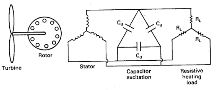
An induction machine can be made to operate as an isolated ac generator by supplying the necessary exciting or magnetizing current from capacitors connected across the terminals of the machine[8, 2, 14]. Fig. 10 shows a typical circuit for a three-phase squirrel-cage induction machine. The capacitors are shown in a delta connection primarily for economic reasons. That is, capacitors built for continuous duty, called motor-run capacitors, are most readily available in 370- and 460-V ratings. Most induction motors in sizes up to 100 kW or more are built with 208-, 230-, or 460-V ratings, so the available capacitors can readily handle the line to line voltages. If the capacitors were reconnected into a wye connection, the voltage across each capacitor is reduced to 1/√3 of the delta connected value, and the reactive power supplied by each capacitor,ωCV2, is then one-third of the reactive power per capacitor obtained from the delta connection. Three times as much capacitance is required in the wye connection, which increases the system cost unnecessarily.
The resistive load is shown connected in wye, but could be connected in delta if desired. There could be combinations of wye and delta connections if different voltage levels were needed.
Figure 10: Self-excited induction generator.
neutral single-phase circuit, as shown in Fig. 11. This is the same circuit shown in Chapter 5, except for the capacitor and load resistor which replace the utility connection. For analysis purposes, the capacitorC is the equivalent wye connected capacitance. That is,
C= 3Cd µF (22)
whereCdis the required capacitance per leg of a delta connection.
This circuit is very similar to that seen in electronics textbooks in a section on oscilla-tors[13]. It is called a negative resistance oscillator. We have a resonant circuit where the capacitive reactance equals the inductive reactance at some frequency, so oscillation will occur at that frequency. Oscillation occurs much more readily when RL is removed, so normal
operation of the induction generator will haveRLswitched out of the circuit until the voltage
buildup has occurred.
The induction generator produces a small voltage from residual magnetism which initiates oscillation. The terminal voltage will build up from this small voltage to a value near rated voltage over a period of several seconds. Once the voltage has reached an operating value, the load resistanceRL can be switched back into the circuit.
It is possible to stop oscillation in any oscillator circuit by excessive load (too small a value of RL). As RL approaches this limit, the oscillator may operate in unexpected modes
due to the nonlinearity of the circuit. The waveform may be bad, for example, or the slip of the induction generator may become unusually large. It should be a part of normal design procedures to determine that the maximum design load for a given generator is not too near this critical limit.
While the general operation of the circuit in Fig. 11 is not too difficult to understand, a detailed analysis is quite difficult because of the nonlinear magnetizing reactance. The available solutions have rather limited usefulness because of their complexity[10, 5, 6, 7]. Detailed reviews of these solutions are beyond the scope of this text, so we shall restrict ourselves to a discussion of some experimental results
Figure 11: Single-phase equivalent circuit of self-excited induction generator.
First, however, we shall discuss some of the features of the machine parameters shown in Fig. 11. This should aid those who need to read the more detailed literature, and should also help develop some intuition for predicting changes in machine performance as operating conditions change.
The circuit quantities R1, R2, Rm, X1,X2, and Xm can be measured experimentally on
a given machine. Techniques for doing this are discussed in texts on electric machinery. It should be mentioned that these machine parameters vary somewhat with operating conditions.
R1 andR2 will increase with temperature between two temperatures Ta and Tb as
Ra
Rb
= 235 +Ta 235 +Tb
(23) where Ta and Tb are in Celsius, Ra is the resistance R1 orR2 at temperature Ta, and Rb is
the resistance atTb. This expression is reasonably accurate for both aluminum and copper,
the common conductors, over the expected range of generator temperatures. The change in resistance from an idle generator at −20oC to one operating on a hot day with winding temperatures of 60oC is (235 + 60)/(235 - 20) = 1.372. That is, the resistancesR1andR2can increase by 37 percent over the expected range of operating temperatures. Such variations would need to be included in a complete analysis.
The resistance Rm represents the hysteresis and eddy current losses of the machine. The
power lost to hysteresis varies as the operating frequency while the eddy current loss varies as the square of the operating frequency. There may also be some variation with operating voltage. The actual operating frequency will probably be between 40 and 60 Hz in a practical system so this equivalent resistor will vary perhaps 40 or 50 percent as the operating frequency changes. If the machine has low magnetic losses so thatRm is significantly greater than the
load resistance RL, then a single average value ofRm would yield acceptable results. In fact,
Rm may even be neglected in the study of oscillation effects if the induction generator has
high efficiency.
The reactancesX1,X2, andXm are given byωL1,ωL2, andωLm whereω is the electrical
radian frequency and L1, L2, and Lm refer to the circuit inductances. The frequency ω will
parameters.
The leakage inductancesL1andL2should not vary with temperature, frequency, or voltage if the machine dimensions do not change. The air gap between rotor and stator may change with temperature, however, which will cause the inductances to change. A decrease in air gap will cause a decrease in leakage inductance.
The magnetizing inductance Lm is a strongly nonlinear function of the operating voltage
VL due to the effects of saturation in the magnetic circuit. In fact, stable operation of this
system is only possible with a nonlinear Lm. The variation of Lm depends strongly on the
type of steel used in the induction generator.
We obtain Lm from a no-load magnetization curve such as those shown in Fig. 12. These
are basically the same curves as the one shown in Fig. 3 for the dc generator except that these are scaled in per unit quantities. The various per unit relationships were defined in Section 5.4. Each curve is obtained under no load conditions (RL=∞) so the slip is nearly zero and
the rotor current I2 is negligible. The magnetizing current flowing through Lm is then very
nearly equal to the output currentI1. The vertical axis is expressed asVL,pu/ωpu, so only one
curve describes operation over a range of frequencies. Strictly speaking, the magnetization curve should be the airgap voltage VA plotted against I1 (or Ie) rather than the terminal
voltage VL. A point by point correction can be made to the measured curve of VL versus I1
by the equation
VA=VL+I1(R1+jX1) (24)
The magnetization curve will have somewhat different shapes for different steels and man-ufacturing techniques used in assembling the generator. These particular curves are for a Dayton 5-hp three-phase induction motor rated at 230 V line to line and 14.4 A and a Baldor 40-hp three-phase induction motor rated at 460/230 V line to line and 48/96 A. Measured parameters in per unit for the 5-hp machine wereRm = 13,R1 = 0.075,R2 = 0.045, and L1
=L2 = 0.16. Measured parameters for the 40-hp machine in per unit wereRm = 21.8, R1 =
0.050, R2 = 0.025, and L1 =L2 = 0.091. The 40-hp machine is more efficient than the 5-hp machine becauseRm is larger and R1 and R2 are smaller, thereby decreasing the loss terms.
We observe that for the 5-hp machine, rated voltage is reached whenI1 is about half the rated current. A terminal voltage of about 1.15 times the rated voltage is obtained for an I1 of about 0.8 times the rated current. It should be noted that it is possible for the magnetizing current to exceed the machine rated current. The magnetizing current needs to be limited to perhaps 0.75 pu to allow a reasonable current flow to the load without exceeding machine ratings. This means that the rated voltage should not be exceeded by more than 10 or 15 percent for the 5-hp self-excited generator if overheating is to be avoided.
The 40-hp machine reaches rated voltage whenI1is about 0.3 of its rated value. A terminal voltage of 130 percent of rated voltage is reached for an exciting current of only 0.6 of rated line current. This means the 40-hp machine could be operated at higher voltages than the
Figure 12: No-load magnetization curves for two induction generators.
5-hp machine without overheating effects. The insulation limitations of the machine must be respected, of course.
The magnetizing current necessary to produce rated voltage should be as small as possible for induction generators in this application. If two machines of different manufacturers are otherwise equal, the one with the smaller magnetizing current should be chosen. This will allow operation with less capacitance and therefore less cost. It may also allow more flexible operation in terms of the operating ranges of load resistance and frequency.
The per unit magnetizing inductanceLm,pu is defined as
Lm,pu= V A,pu
ωpuIm,pu
(25) An approximation forLm,pu which may be satisfactory in many cases is
Lm,pu VL,pu
ωpuI1,pu
(26) This is just the slope of a line drawn from the origin of Fig. 12 to each point on the
magne-tization curve. Approximate curves for Lm,pu for the two machines are presented in Fig. 13.
We see that the inductance is constant for voltages less than about one-half of rated. The inductance then decreases as saturation increases.
Figure 13: Per unit magnetizing inductance as a function of load voltage.
We see that any detailed analysis is made difficult because of the variability of the ma-chine parameters. Not only must a nonlinear solution technique be used, the solution must be obtained for the allowable range of machine parameters. This requires a great deal of computation, with the results being somewhat uncertain because of possible inadequacy of the machine model and because of inadequate knowledge of the parameter values. We shall leave such detailed analyses to others and turn now to an example of experimental results.
Figure 14 shows the variation of terminal voltage with input mechanical power for the 40-hp machine mentioned earlier. The rated voltage is 230 V line to line or 132.8 V line to neutral. Actual line to neutral voltages vary from 90 to 150 V for the data presented here.
Figure 14: Variation of output voltage with input shaft power for various resistive and capac-itive loads for a 40-hp self-excited induction generator.
All resistance was disconnected from the machine in order to establish oscillation. Once a voltage close to rated value was present the load was reconnected and data collected. Voltage buildup would not occur for speed and capacitance combinations which produce a final voltage of less than 0.8 or 0.9 of rated. For example, with 285µF of capacitance line to line, the voltage would not build up for speeds below 1600 r/min. At 1600 r/min the voltage would slowly build up over a period of several seconds to a value near rated. The machine could then be operated at speeds down to 1465 r/min, and voltages down to 0.7 of rated before oscillation would cease.
The base power for this machine is √3(230 V)(96 A) = 38,240 W. The rated power is
√
3(230)(96) cosθ, which will always be smaller than the base power. Because of this feature of the per unit system, the mechanical input power should not exceed 1.0 pu except for very short periods because the machine is already overloaded atPm = 1.0 pu. The base impedance
is 132.8/96 = 1.383 Ω. The base capacitance is 1/(Zbaseωbase) = 1/[(1.383)(377)] = 1918µF line to neutral. A line to line capacitance of 385µF, for example, would be represented in our analysis by a line to neutral capacitance of 3(385) = 1155 µF, which has a per unit value of 1155/1918 = 0.602 pu. A good starting point for the capacitance on experimental induction generators in the 5-50 hp range seems to be about 0.6 pu. Changing capacitance will change performance, but oscillation should occur with this value of capacitance.
Returning to our discussion of Fig. 14, we see that for curve 1, representing a load of 2.42 pu and a capacitance of 0.602 pu, the voltage varies from 0.68 pu to 1.13 pu asPmvaries from
0.22 pu to 0.59 pu. The variation is nearly linear, as would be expected. When the resistance is decreased to 1.39 pu with the same capacitance, we get curve 2. At the samePm of 0.59 pu,
the new voltage will be about 0.81 pu. The electrical power out,VL2/RL, will remain the same
if losses do not change. We see that the voltage is determined by the resistance and not by the capacitance. Curves 2 and 3 and curves 4 and 5 show that changing the capacitance while keeping resistance essentially constant does not cause the voltage to change significantly.
Changing the capacitance will cause the frequency of oscillation to change and therefore the machine speed. We see how the speed varies withPmin Fig. 15. A decrease in capacitance
causes the speed to increase, for the same Pm. The change will be greater for heavy loads
(smallRL) than for light loads. The speed will also increase with Pm for a given RL and C.
The increase will be rather rapid for light loads, such as curves 4 and 5. The increase becomes less rapid as the load is increased. We even have the situation shown in curve 7 where power is changing from 0.4 to 0.6 pu with almost no change in speed. The frequency will change to maintain resonance even if the speed does not change so we tend to have high slip where the speed curves are nearly horizontal. For this particular machine the efficiency stayed at about 90 percent even with this high slip and no other operational problems were noted. However, small increases in load would cause significant increases in speed, as seen by comparing curves 6 and 7. It would seem therefore, that this constant speed-high slip region should be avoided by adding more capacitance. Curves 7, 3, and 2 show that speed variation becomes more pronounced as capacitance is increased from 0.446 pu to 0.602 pu. We could conclude from this argument that a capacitance of 0.524 pu is the minimum safe value for this machine even though a value of 0.446 pu will allow operation.
We now want to consider the proper strategy for changing the load to maintain operation under changing wind conditions. The mechanical power output Pm from the wind turbine
is assumed to vary from 0 to 1.0 pu. A capacitance value of 0.524 is assumed for discussion purposes. AtPm = 1.0 pu the voltage is 1.09 pu and the speed is 1.01 pu for RL = 1.38 pu.
These are good maximum values, which indicate that good choices have been made for RL
andC. As input power decreases to 0.44 pu the speed decreases to 0.944 pu. If input power is decreased still more, the induction generator gets out of the nonlinear saturation region and
oscillation will cease. We therefore need to decrease the load (increaseRL). Note that there
is a gap between curves 3 and 4, so we may have a problem if we change fromRL = 1.38 pu
to 4.66 pu. The voltage will be excessive on the larger resistance and we may lose oscillation with the smaller resistance, while trying to operate in the gap area. We need an intermediate value ofRL such that the curve for the larger RL will intersect the curve for the smaller RL,
Figure 15: Variation of rotational speed with input shaft power for various resistive and capacitive loads for a 40-hp self-excited induction generator.
Curves 1 and 2 intersect at Pm = 0.5 pu so we can visualize a curve for a new value of
RL that intersects curve 3 at the same Pm. This is shown as curve 4 in Fig. 16. If we are
operating on curve 4 atPm= 0.2 pu, the speed is about 0.8 of rated. As shaft power increases
to Pm = 0.5 pu the speed increases to about 0.95 of rated. Additional load can be added
at this speed without causing a transient on the turbine since power remains the same. The speed then increases at a slower rate to 1.01 pu atPm = 1.0 pu. If the wind is high enough
to produce even greater power, the propeller pitch should be changed, brakes set, or other overload protection measures taken.
Figure 16: Variation of rotational speed with input shaft power for three well-chosen resistive loads for a 40-hp self-excited induction generator.
RL= V 2 L Pe = V 2 L ηgPm (27) We are assuming an ideal transmission between the turbine and the generator so the turbine power output is the same as the generator input. If we want actual resistance, we have to use the voltage and power values per phase. On the per unit system, we use the per unit values directly. For example, forVL = 1.0 pu on curve 3 in Fig. 14, we readPm = 0.86 pu. If RL =
1.38 pu, thenPe = (1.0)2/1.38 = 0.72. ButPe =ηgPm soηg = 0.72/0.86 = 0.84, a reasonable
value for this size machine. If we assumeVL = 1.15, Pm = 0.5, andηg = 0.84 for the curve
4, we find RL = (1.15)2/(0.84)(0.5) = 3.15 pu.
This value ofRLwill work for input power levels down to aboutPm = 0.2 pu. For smaller
Pm we need to increase RL to a larger value. We can use the same procedure as above to
get this new value. If we assume a point on curve 8 of Fig. 16 where VL = 1.15 pu, Pm =
0.5 pu, and ηg arbitrarily assumed to be 0.75, we find RL = (1.15)2/(0.75)(0.2) = 8.82 pu.
This resistance should allow operation down to aboutPm = 0.08, which is just barely enough
to turn the generator at rated speed. Speed and voltage variations will be substantial with this small load. There will probably be a mechanical transient, both as the 8.82 pu load is switched in during startup, and as the load is changed to 3.15 pu, because the speed versus power curves would not be expected to intersect nicely as they did in the case of curves 3 and 4. These transients at low power levels and light winds would not be expected to damage the turbine or generator.
We see from this discussion that the minimum load arrangement is the one shown in Fig. 17. The switches S1,S2, and S3 could be electromechanical contactors but would more probably be solid state relays because of their speed and long cycle life. The control system could operate on voltage alone. As the turbine started from a zero speed condition,S1 would be closed as soon as the voltage reached perhaps 1.0 pu. When the voltage reached 1.15 pu, implying a power output of Pm = 0.2 pu in our example, S2 would be closed. When the
voltage reached 1.15 pu again, S3 would be closed. When the voltage would drop below 0.7 pu, the highest numbered switch that was closed would be opened. This can be done with a simple microprocessor controller.
6 SINGLE-PHASE OPERATION OF THE
INDUCTION GENERATOR
We have seen that a phase induction generator will supply power to a balanced three-phase resistive load without significant problems. There will be times, however, when single-phase or unbalanced three-single-phase loads will need to be supplied. We therefore want to examine this possibility.
Single-phase loads may be supplied either from line-to-line or from line-to-neutral voltages. It is also possible to supply both at the same time. Perhaps the most common case will be the rural individual who buys a wind turbine with a three-phase induction generator and who wants to sell single-phase power to the local utility because there is only a single-phase distribution line to his location. The single-phase transformer is rated at 240 V and is center-tapped so 120 V is also available. The induction generator would be rated at 240 V line to line or 240/√3 = 138.6 V line to neutral. The latter voltage is too high for conventional 120-V equipment but can be used for heating if properly rated heating elements are used.
A circuit diagram of the three-phase generator supplying line-to-line voltage to the utility network and also line-to-line voltage to a resistive load is shown in Fig. 18. Phasesa and b
are connected to the single-phase transformer. Between phaseband phasecis a capacitor C. Also shown is a resistorRLwhich can be used for local applications such as space heating and
domestic water heating. This helps to bring the generator into balance at high power levels. It reduces the power available for sale to the utility at lower power levels so would be placed in the circuit only when needed.
The neutral of the generator will not be at ground or earth potential in this circuit, so should not be connected to ground or to the frame of the generator. Some induction generators will not have a neutral available for connection because of their construction, so this is not a major change in wiring practice.
The induction generator will operate best when the voltagesVa,Vb, andVcand the currents
Ia,Ib, andIcare all balanced, that is, with equal magnitudes and equal phase differences. Both
voltages and currents become unbalanced when the generator supplies single-phase power. This has at least two negative effects on performance. One effect is a lowered efficiency. A machine which is 80 percent efficient in a balanced situation may be only 65 or 70 percent efficient in an unbalanced case. The other effect is a loss of rating. Rated current will be reached in one winding well before rated power is reached. The single- phase rated power would be two thirds of the three-phase rating if no balancing components are added and if the efficiency were the same in both cases. Because of the loss in efficiency, a three-phase generator may have only half its three-phase rating when connected directly to a single-phase transformer without the circuit componentsC and RL shown in Fig. 18.
It is theoretically possible to chooseC andRLin Fig. 18 so that the induction generator is
Figure 18: Three-phase induction generator supplying power to a single-phase utility trans-former.
The phasor diagram for the fully balanced case is shown in Fig. 19. In this particular diagram, the capacitor is supplying all the reactive power requirements of the generator. This allows
Ia to be in phase withVab so only real power is transferred through the transformer. In the
fully balanced case, Ib and Ic must be equal in amplitude toIa and spaced 120o apart, which
puts them in phase with Vbc and Vca. The current IR is in phase with Vbc and IX leads Vbc
by 90o. By Kirchhoff’s current law,IR+IX =−Ic. When we draw the necessary phasors in
Fig. 19, it can be shown that|IR| = 0.5|Ia| and |IX|= 0.866|Ia|. If we had a constant shaft
power, such as might be available from a low head hydro plant, and if we had some use for the heat produced in RL, then we could adjustC and RL for perfect balance as seen by the
generator and for unity power factor as seen by the utility. The power supplied to the utility isVabIaand the power supplied to the local load is 0.5VabIa, so two-thirds of the output power
is going to the utility and one-third to the local load.
Unfortunately, a given set of values only produce balanced conditions at one power level. As the wind speed changes, operation will again be unbalanced. It is conceptually possible to have a sophisticated control system which would be continually changing these components as power level changes in order to maintain balance. This system could easily be more expensive than the generator and make the entire wind electric system uneconomical. We, therefore, are interested in a relatively simple system where one or more switches or contactors are controlled by rather simple sensors and logic circuitry. Hopefully, efficiency and unbalance will be acceptable over the full range of input power with this simple system. Capacitance and resistance would be added or subtracted as the power level changes, in order to maintain these acceptable conditions.
Perhaps the simplest way to illustrate the imbalance effects is with an example. Figure 20 shows the variation of the line to line voltages and the line currents for the 40-hp induction
Figure 19: Phasor diagram for circuit in Fig. 18 at balanced operation at unity power factor. generator described in the previous section. The capacitance C = 0.860 pu (actual value is 550µF). The resistanceRLwas omitted so all the power is being delivered to the utility. The
generator voltage of 230 V line to line is used as the base, but the available utility voltage was actually a nominal 208 V. This explains why Vab always has a value less than 1.0 pu, since
the utility connection did not allow the generator voltage to reach 230 V.
At values ofPmnear zero, the currentIabeing supplied to the utility is also near zero. This
forcesIb andIc to have approximately the same magnitudes. As Pm increases, Iaincreases in
an almost linear fashion. The voltage Vbc across the capacitor and the current Ic through it
remain essentially constant. The current in phasebdecreases at first and then increases with increasing Pm. The voltage Vab to the transformer increases from 0.92 pu to 0.99 pu as Pm
increases, due to voltage drops in the transformer and wiring.
The currentIa reaches the machine rating at a value ofPm of about 0.6 pu. As mentioned
earlier, a generator should supply up to two-thirds of its three-phase rating to a single-phase load, but because of lower efficiency the generator limit will be reached at a slightly lower value. For this particular machine, the three-phase electrical rating is about 32,500 W. Rated current was reached at 21,000 W as a single-phase machine or 0.646 of the three-phase rating. This is just slightly under the ideal value of 0.667.
The efficiency drops if a larger capacitor is used. This increasesIc, which increases ohmic
losses in that winding without any compensating effect on the losses due to imbalance. A value ofIc of about half of rated seemed to give the best performance over this range of input
power. This makes its value close to the average values of Ia and Ib for this range of Pm,
which is probably close to the optimum value.