A Queueing-Theoretic Foundation of Available
Bandwidth Estimation: Single-Hop Analysis
Xiliang Liu
, Member, IEEE
, Kaliappa Ravindran, and Dmitri Loguinov
, Member, IEEE
Abstract—Most existing available-bandwidth measurement techniques are justified using a constant-rate fluid cross-traffic model. To achieve a better understanding of the performance of current bandwidth measurement techniques in general traffic conditions, this paper presents a queueing-theoretic foundation of single-hop packet-train bandwidth estimation under bursty arrivals of discrete cross-traffic packets. We analyze the statistical mean of the packet-train output dispersion and its mathematical relationship to the input dispersion, which we call the probing-re-sponse curve. This analysis allows us to prove that the single-hop response curve in bursty cross-trafficdeviatesfrom that obtained under fluid cross traffic of the same average intensity and to demonstrate that this may lead to significant measurement bias in certain estimation techniques based on fluid models. We conclude the paper by showing, both analytically and experimentally, that the response-curve deviation vanishes as the packet-train length or probing packet size increases, where the vanishing rate is decided by the burstiness of cross-traffic.
Index Terms—Active measurement, bandwidth estimation, packet-pair sampling.
I. INTRODUCTION
A
VAILABLE bandwidth of a network path has long been the interest of measurement studies because of its impor-tance to many Internet applications such as overlay routing, server selection, congestion control, and network diagnosis. Several measurement techniques have been developed over the last few years, among which TOPP [17], pathload [8], PathChirp [23], IGI/PTR [6], and Spruce [24] are the major representatives. Most of the current proposals are based on packet-pair or packet-train probing, where bursts of equally spaced packets of uniform size are injected into the path of in-terest, and the available bandwidth information is inferred from the relationship between input/output inter-packet dispersions.According to a commonly accepted notion, the available bandwidth of a network hop is itsresidualcapacity after trans-mitting cross traffic. Since at any time instant, the hop is either idle or transmitting packets at its capacity , the instantaneous link utilization can be viewed as an ON–OFFfunction of time, i.e., if the link is idle at time and
if the link is busy transmitting a packet at time . The average
Manuscript received August 15, 2005; revised June 13, 2006; approved by IEEE TRANSACTIONS ONNETWORKINGEditor D. Veitch. This work was sup-ported by NSF Grants CCR-0306246, ANI-0312461, 0434940, and CNS-0519442.
X. Liu is with Bloomberg L.P., New York, NY 10022 USA (e-mail: [email protected]).
K. Ravindran is with the Computer Science Department, City College of New York, New York, NY 10031 USA (e-mail: [email protected]).
D. Loguinov is with the Computer Science Department, Texas A&M Univer-sity, College Station, TX 77843 USA (e-mail: [email protected]).
Digital Object Identifier 10.1109/TNET.2007.896235
utilization of the hop during time interval is then given by
(1) Thehop available bandwidth in is the average unutilized capacity of the hop within that interval, i.e.,
(2) Theavailable bandwidth of a network pathis the minimum available bandwidth of all traversed links. The link carrying the minimum available bandwidth is called thetight link.
Note that varies over time as well as over a wide range of observation intervals . These dynamics make it an elusive target to measure. To combat this difficulty, most ex-isting bandwidth-measurement approaches use a constant-rate fluid cross-traffic model to justify the design of their estima-tion techniques. Under such fluid1cross-traffic, becomes
a constant for all , and all and its relationship to the probing input and output becomes easy to identify.
Although the experimental performance of recent proposals as documented is encouraging, the rationale they are anchored upon is not fully justified in general cross-traffic conditions. To better understand the behavior and performance of existing techniques, this paper presents a queueing-theoretic analytical framework that allows an in-depth analysis of the asymptotic behavior of single-hop packet-train bandwidth estimation under bursty arrivals of discrete cross-traffic packets. Our analysis ad-dresses two fundamental issues. First, given a cross-traffic arrival process and fixed packet-train parameters (i.e., packet size and train length), we demonstrate how the probing output relates to the probing input. We investigate the output rate and dispersion of individual packet-trains as well as their asymptotic average as the number of packet-train samples approaches infinity. We examine the functional dependency between the input and the asymptotic average of the output in the entire input range. We call this relationship theprobing-response curveand show how the available bandwidth information is embedded in it. Second, we investigate how the response curve evolves with respect to the changes in packet train parameters and cross-traffic burstiness. Both questions are of central importance for the design of available-bandwidth estimation methods. The answer to the first question provides a theoretical foundation that extends the pre-vious rationale based on fluid cross-traffic models. The answer to the second question offers an insight into parameter tuning strategies in the design of future measurement techniques. Even though published research has produced a great deal of intuition
1We use the terms “constant-rate fluid” and “fluid” interchangeably.
and empirical findings related to these questions, a mathemat-ically precise explanation of the bandwidth sampling process was not available until now.
While the eventual goal of our analysis is to understand packet-train bandwidth estimation in multihop network paths, single-hop results are indispensable in reaching this goal. Moreover, the single-hop case on its own is an interesting and complex problem calling for an elaborate discussion, which is the focus of this paper. We extend the discussion to multihop paths in a separate paper [14].
Under a theoretically and practically mild assumption, we de-rive several important properties of the gap (and rate) response curve. Our results show that the gap response curve in con-stant-rate fluid cross traffic is the tight lower bound of that in bursty cross traffic with the same average intensity. We show that there is an input dispersion range where the real curve pos-itively deviates from its fluid-based prediction. Most existing proposals were designed without being aware of the response deviation phenomenon, which sometimes makes them subject to significant measurement bias.
Our analysis also discovers the source of this deviation and arrives at its closed-form expression in the packet-pair case. We show that the amplitude of the response deviation is exclusively decided by the packet-train parameters and the available band-width distribution and that it vanishes as probing packet size or packet-train length increases. We also present an experimental approach to compute with high accuracy the response curves from a given cross-traffic trace. This allows us to empirically validate our theoretical results, qualitatively observe the rela-tionship between the response deviation and packet-train param-eters in certain cross-traffic conditions, and evaluate the asymp-totic performance of various available-bandwidth estimators.
The rest of the paper is organized as follows. In Section II, we summarize the current measurement proposals and the fluid models they are based upon or related to. In Section III, we present our analytical framework of packet-train bandwidth es-timation. Using this framework, we analyze major properties of the response curves and the response deviation phenomenon in Section IV. We provide numerical results of the response devi-ation and examine its reldevi-ationship to several deciding factors in Section V. We explain the implications of our findings on some of the current proposals in Section VI. Finally, we present con-cluding remarks in Section VII.
II. BACKGROUND
IP-layer bandwidth estimation using packet-pairs originates from the seminal work by Bolot [3], Jacobson [7], Keshav [10]. However, due to a lack of consensus on what available band-width was and how to measure it, most of the original research efforts in this area went into the measurement of bottleneck ca-pacity [4], [11], [21]. The recent surge of available-bandwidth estimation proposals stems from the fluid model developed in bottleneck capacity estimation research [4], [17]. In what fol-lows, we first briefly introduce this fluid model and then show how the current techniques are related to it.
A. Fluid Model
Consider a single-hop path with capacity and assume that cross traffic is a fluid with constant arrival rate . This fluid
assumption means that for any time interval, the amount of cross traffic arriving at the link is . The available bandwidth of the path is , regardless of the observation time instant or the observation time interval. Consider a probing train of packets with equal interpacket dispersion and packet size that passes though the path. The output dispersion can be expressed by the following piecewise linear function of :
(3) Using packet-pairs (i.e., ), the practical meaning of (3) is as follows. The first packet arrives into the hop at time and experiences zero queueing delay due to the fluid nature of cross traffic. Hence, it departs from the hop at time
. The second packet arrives into the hop at time . Before the hop can serve , the amount of data it has to transmit during the time interval is . If this is done before arrives, i.e., , then also experiences zero queueing delay, and we obtain . Otherwise, the hop undergoes a busy period between the departures of the two
packets and the output dispersion is . A
similar argument applies to packet-trains of any length. Model (3), which we term thesingle-hop fluid gap response curve, has several variants that exhibit more direct associations with available-bandwidth estimation. One such variant is the rate response curve depicting the functional relationship be-tween the input probing rate and the output rate
:
(4) Since the rate response curve is not linear, Melanderet al.. proposed in [17] to use a transformed version of (4), which de-picts the relation between and :
(5) We next explain how various types of bandwidth information is embedded in fluid response curves. First, note that each of the three fluid curves contains two segments and that the input rate at the turning point between the two segments is equal to the available bandwidth of the path, i.e., . Second, observe that the segment in the input rate range carries information about hop capacity and cross-traffic arrival rate . We next discuss how current techniques are designed to extract available bandwidth from fluid response curves.
B. Measurement Techniques
Recently, Jain and Dovrolis presented a classification of ex-isting measurement techniques [9]. Techniques that use a single input rate are calleddirectand those using multiple input rates are callediterative.
Several direct probing methods are Delphi [22], IGI [6], Spruce [24], and the work in [5]. These approaches use one point of the response curve where the input rate is higher than the available bandwidth. They assume that the hop ca-pacity is known or can be measured separately (e.g., using existing capacity estimation tools such as path rate). Hence, every packet-train sample of these methods can generate an
estimate of the cross-traffic arrival rate during the sampling interval , where is the arrival time of the first packet in a train to the tight link. These tools obtain a final estimate of by averaging multiple probing samples, and the available bandwidth is computed by subtracting the estimated cross-traffic arrival rate from the known link capacity . Direct probing methods differ among each other in the input probing rate they choose, packet-train parameters, and the assumptions they make on cross-traffic.
Representative iterative methods are TOPP [17], pathload [8], and PTR [6]. Iterative methods do not assume the knowledge of link capacity. They send packet-trains at multiple input probing rates, either to locate the turning point in the response curve (e.g., pathload and PTR) or to extract both and from the linear segment in the input rate range (e.g., TOPP). Note that compared to PTR, pathload locates the turning point by de-tecting a trend of increasing one-way delay among the probing packets in a train, instead of comparing the output rate of the packet-train to its input rate. Hence, even though pathload is re-lated to the fluid response curves presented previously, it is not directly based upon them.
C. Discussion
We make several observations regarding the current measure-ment techniques to motivate our subsequent analysis. First, note that in bursty cross traffic, both the available bandwidth and cross-traffic arrival rate may exhibit a great deal of statistical variability. Most existing techniques produce a single numer-ical result for each run, which is interpreted as the average avail-able bandwidth within the measurement duration.2Second,
cur-rent techniques assume that cross-traffic burstiness only causes measurement variability, which can be smoothed out by aver-aging multiple probing samples. This means that when a large number of packet-train samples are used, the fluid model be-comes a valid first-order approximation of the real stochastic process. This assumption can be formalized as the following equality:
(6) where term is the statistical mean (or asymptotic average) of output dispersions when a large number of packet-train sam-ples are used. The term should be viewed as the long-term av-erage arrival rate of cross-traffic since a large number of packet-train samples naturally extends the measurement duration to a long time period.
However, there has been no analytical investigation regarding the validity of (6) in general traffic conditions. A positive an-swer to this question would lay a solid ground for the design of available-bandwidth measurement tools and provide them with an assurance of asymptotic accuracy. On the other hand, a nega-tive answer would shed new light on the fundamental limits and tradeoffs in probing-based measurement and give rise to new in-sights into parameter tuning under diverse application require-ments. To tackle this question, we present the necessary analyt-ical framework in the next section.
2Note that pathload is an exception in the sense that it produces a variation
range of the-interval available bandwidth within the measurement duration, where = (n 0 1)g is the sampling interval of each packet-train.
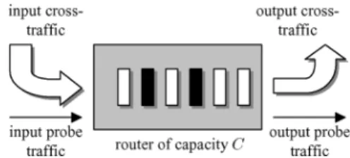
Fig. 1. Single-hop probing model.
III. ANALYTICALFRAMEWORK OFPACKET-TRAINPROBING
This paper is an extension of our previous work [12]. Due to limited space, the proofs of several lemmas and theorems are presented in [13] and are omitted from this paper.
We present our analytical framework in four steps. First, we define a set of random processes that model cross-traffic arrival and hop available bandwidth. Second, we introduce a concept we callprobing intrusion residualto characterize the interaction between probing packets and cross traffic. Using these defini-tions, we derive in the third step a mathematical relationship be-tween input and output packet-train dispersions. This result calls for a certain understanding of the underlying processes sampled by packet-train arrivals, which is the task of our final step.
A. Cross-Traffic Arrival
Our analysis focuses on the single-hop probing model in Fig. 1. We assume infinite buffer space inside the router, a work-conserving FIFO queueing discipline, andsimpletraffic arrival (i.e., at most one packet arrives at any time instant). We next identify a set of random processes that play a crucial role in modeling packet-train probing.
Definition 1: Cross-traffic is driven by the packet-counting
process and the packet-size process
. The cumulative traffic arrival is a random process counting the total volume of data3received by the hop up to time instant :
Note that and are right continuous, meaning that the packet arriving at is counted in .
Definition 2: We define as the average
cross-traffic arrival rate in the interval :
and call it the -interval cross-traffic intensity process.
Definition 3: At time instant , the hop-workload process
is the sum of service times of all packets in the queue and the remaining service time of the packet in service.
Definition 4: We define to be the dif-ference between hop workload at times and :
and call it the -interval workload-difference process. 3In this paper, packet size and data are measured in bits.
Definition 5: Thehop utilization process
is anON–OFFprocess associated with :
(7) and the -interval hop idle process
(8) is the total amount of idle time of the forwarding hop in . We further call time interval hop busy periodif
andhop idle periodif .
Definition 6: We define as the residual bandwidth in the time interval :
(9) and call it the -interval available bandwidth process.
The following lemma describes the relationship among the
three important processes and .
Lemma 1: For all positive and , the following holds: (10) Bandwidth estimation is essentially interaction of probe packets withsample-pathsof the processes we just defined. We next examine certain properties of this interaction.
B. Probing Intrusion of Packet Trains
We use quadruple to denote a probing train of packets , where is the arrival time of the first packet at the hop, is the interpacket dispersion at the sender, is the probe packet size, and is the train length. Ar-rival times of probing packets to the hop are denoted by
. Departure times of probing packets from the hop are denoted by . We de-fine theoutput gapof a packet train as theaveragedispersion between adjacent packets in the train:
(11) In terms of rate, the input and output probing rates are
and .
We use and to respectively denote sample paths of workload and hop idle time processes associated with the perposition of cross traffic and probing traffic. Note that this su-perposition only increases hop workload, i.e., for all
. We next define more useful notation to help us examine this intrusion behavior of packet train probing.
Definition 7: Theintrusion rangeof probing traffic into is the set . Theintrusion residual function
is .
Function helps us understand the intrusion behavior of the probing traffic into . Before the arrival of probing packets, . Upon every arrival of a probe packet, gets an immediate increment of , where is the probing packet size as before. In ’s busy periods without additional probing packet arrival, remains unchanged. In
Fig. 2. Illustration of intrusion residual function.
’s idle periods without additional arrival of probe packets, deceases linearly with slope . Function is monotonically nonincreasing between every two adjacent probing packet arrivals. Fig. 2 illustrates this behavior, where
and are two busy periods in , and
and are two idle periods in . Times and
are the instants of probing packet arrivals. Time is the end point of the intrusion range.
Based on the above observations and assuming a single probe packet of size arrives to the hop at time can be ex-pressed as follows:
(12) When the hop is probed by a packet train , we are often interested in computing function
(13)
for , where denotes the left-sided limit
. Metric 4is the intrusion residualcaused
by the first packets in the probing train and
experiencedby packet . In other words, the queueing delay of in the hop is given by
(14) The total sojourn time of at the hop is the sum of its service time and its queueing delay
(15) As a direct result of (12), can be recursively computed as follows:
(16) As shown in (14), the introduction of intrusion residual sep-arates the queueing delay of a probing packet into two portions with different statistical nature. This is one of our key results that make in-depth analysis of packet-train bandwidth estima-tion possible.
C. Output Dispersion of Individual Packet-Trains
Our next lemma expresses the output dispersion of a packet-train from two different angles. This result is the corner stone of our later response-curve analysis.
Lemma 2: Let . When a hop with
work-load process is probed by a packet train , the output gap can be expressed as
(17) The most interesting feature of Lemma 2 is that its result is unconditional, in the sense that it neither relies on any as-sumption on the cross-traffic arrival pattern nor imposes any restriction on packet-train parameters. In addition, Lemma 2 develops an avenue towards analytical understanding of the re-sponse curve through (especially first-order) statistical proper-ties of each individual terms in (17).
Also note that the four terms , , and
in (17) are generated by sampling four underlying
con-tinuous-time sample paths , and at
time instant . Hence, before examining the random samples generated by packet-train probing, we first have to understand several important statistical properties of the underlying contin-uous-time processes being sampled.
D. Properties of Underlying Processes
We first make an assumption on cross-traffic arrival.
Assumption 1: There exists a constant less than hop
ca-pacity such that as .
This assumption has a series of implications, First, it states that the cross-traffic has a long-term average arrival rate . This further leads to the following result.
Lemma 3: The limiting time-average of any -interval cross-traffic intensity sample path is equal to
(18)
Proof: First, notice that
(19)
Computing the limits, we get
(20)
Since is a nondecreasing function, we can write
(21)
Finally, note that both and have the same limit when divided by :
(22) Combining (20) and (22), we have for
(23) which leads to the statement of the lemma.
Throughout this paper, we adopt sample-path arguments and use the notation of probability expectation as a shorthand repre-sentation for sample-path limiting time-average.5Note that the
first equality in Lemma 3 is by definition and has nothing to do with ergodicity.
The second important implication of Assumption 1 is the workload stability of the forwarding hop.
Lemma 4: Given Assumption 1, the forwarding hop exhibits
workload stability, i.e., .
Proof: See Appendix I.
An immediate consequence of workload stability is the zero-mean nature of , formally stated as follows.
Lemma 5: If , the limiting time average of any -interval workload-difference sample path is zero:
(24) The next two results concern the available bandwidth process . Although does not explicitly appear in (17), it is functionally related to two processes and . Further-more, the process is important on its own right as it is the target of our measurement.
Lemma 6: Under the assumptions of this paper, -interval available bandwidth converges to as the observation in-terval becomes large:
(25) This result implies that a “good” measurement technique should produce as its final estimate given a sufficiently long measurement duration.
Lemma 7: The limiting time-average of any -interval avail-able bandwidth process is , i.e.,
(26) This result shows that first-order statistics of an available bandwidth sample path do not depend on the observation interval and equal the average long-term available bandwidth. 5The limiting time-average of a sample path is the expectation of its limiting
frequency distribution [19, pp. 45–50]. Hence, it is also called the “sample-path mean.”
On the other hand, note that any higher order sample-path statistics of have a strong dependence on . We define a function to describe the available bandwidth distribution along sample path :
(27) In general, we can assume that the frequency distribution function converges to the following step function as
:
(28) We finish the section by deriving useful bounds on the re-maining two terms and in (17) and leave their detailed investigation for the next section. From (16), noticing that is no less than zero and applying mathematical
induction to , we get . Combining with
Lemma 2, we have.
Corollary 1: Let . Then, the following inequal-ities hold:
(29) where the second inequality is tight iff .
Our next lemma provides a bound for the term .
Lemma 8: Let . Then, we have
(30)
Collecting Lemmas 2 and 8 leads to the following result.
Corollary 2: When is probed by packet train , the following holds:
(31) With the basic analytical framework established in this sec-tion, we are now in a position to derive the probing-response curve of a single-hop path.
IV. PROBING-RESPONSECURVES
The probing-response curve depends on a number of fac-tors such as packet-train parameters, intertrain delay pattern, and cross-traffic characteristics. We assume a Poisson arrival of probe trains to the hop, because the asymptotic average of Poisson samples converges to the limiting time average of the sample path being sampled. This property is known as PASTA (Poisson arrivals see time averages) [25]. The average rate of Poisson sampling is assumed to be small enough so that depen-dency between adjacent trains can be neglected.
We use to denote a probing train series
driven by a Poisson arrival process
. We use to denote the output gap of the th probing train
in the series, i.e., .
The limiting average of the discrete-time sample-path is given by
(32) We next derive several bounds on the response curve, show examples of applying these bounds, and study packet-train pa-rameter effect on the deviation of the response curve from its fluid bound.
A. Bounds
We first obtain the upper and lower bounds on the gap re-sponse curve.
Theorem 1: When is probed by a Poisson packet-train
series , the following holds:
(33)
Proof: Let . Then, using Corollary 2,
con-dition implies
(34) Since is driven by Poisson arrivals, we have the following due to the PASTA property:
(35) Combining (34), (35), and Lemma 3, we get (33).
Rearranging the result of Theorem 1, we get
(36) which explains when and why the term can form an unbiased estimator of cross-traffic intensity. We note that this traffic intensity formula is used by several techniques and plays an important role in available bandwidth estimation.
Theorem 2: When is probed by Poisson packet-train
series , the following holds:
Proof: Notice that from Corollary 2, when
(37) Similarly, from Corollary 1, PASTA, and Lemma 5, we have
(38) Collecting (37) and (38), we get
For the upper bound, from Corollary 2, PASTA, and Lemma 3, we get
(40) Then, from Corollary 1, PASTA, and Lemma 5, we obtain
(41) Combining (40) and (41), we get
(42) Combining (39) and (42), the theorem follows.
Theorem 2 provides lower and upper bounds on when . Combining this result with the one in Theorem 1 for , we get a lower bound on in the entire probing
range as follows:6
(43)
This is exactly model (6) we are trying to validate. However, Theorem 2 shows that (6) is alower boundof , which does not necessarily equal to . Likewise, we can obtain from the two theorems the entire upper bound of as follows:
(44)
The real gap response curve is contained between these two bounds. We define the response deviation as the difference between the real gap response curve and the lower bound given by (43). It can be expressed by the following using Theorem 2, Lemma 2, and PASTA (where ):
(45)
We next provide a closed-form expression for the packet-pair (i.e., ) response deviation to gain additional insight into the nature of this phenomenon.
6FunctionsL(f)andU(f)denote lower and upper bound onf, respectively.
B. Packet-Pair Closed-Form Expression
Notice that both and can be expressed as deter-ministicfunctions whose arguments are packet-train parameters and the following -dimensional vector:
(46)
In particular, when is simply and the vector (46) degenerates to a scalar, which allows us to obtain simple
expressions for and :
(47) (48) Consequently, we have the following result regarding the packet-pair probing-response curve.
Theorem 3: Assuming that is probed by Poisson
packet-pair series , let and denote
by the frequency distribution function of sample-path process . Then, the following holds:
(49) It immediately follows that the packet-pair response deviation is
(50)
The response deviation phenomenon is one of the previously unknown factors that can cause measurement bias for available bandwidth estimation techniques based on (6). Even though a closed-form expression of the response deviation for packet-trains is complex in general, it is clear that the amount of devi-ation is exclusively decided by the packet-train parameters
and the sample-path frequency distribution of the available bandwidth vector (46).
Next, we show the full picture of response curves for both gap-based and rate-based versions.
C. Full Picture
We now investigate the relationship between the response de-viation given in (45) and the input gap while keeping all other parameters fixed. We first examine packet-pair probing.
Theorem 4: When is probed by Poisson packet-pair
se-ries , the response deviation equals
zero when input gap ; it is a monotonically in-creasing function of in the input gap range ; and it is a monotonically decreasing function of in the input
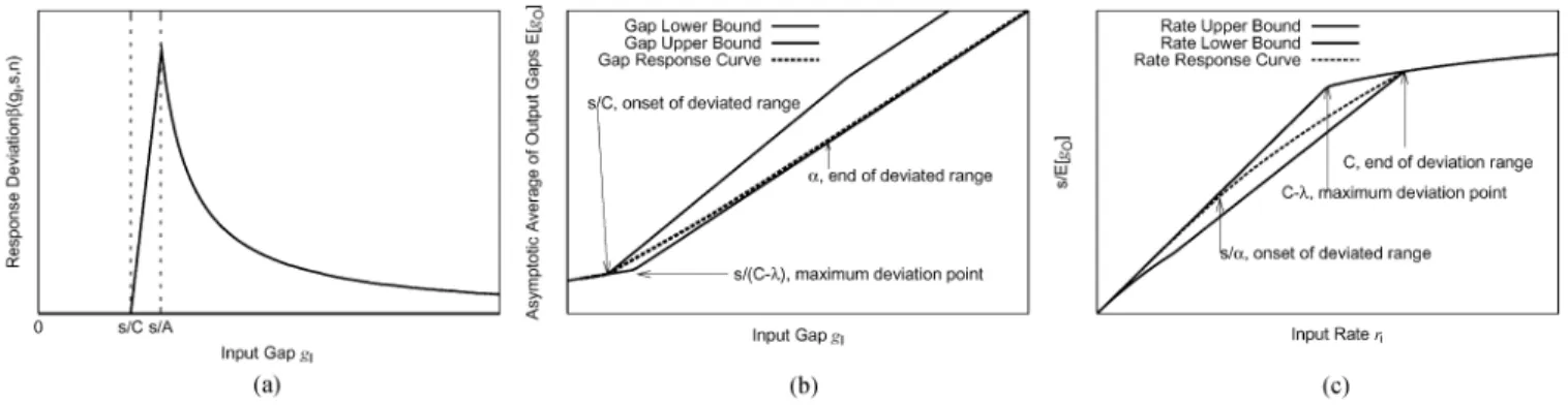
Fig. 3. Illustration of various properties of response curves in the entire input range. (a) Response deviation, (b) gap-response curve, and (c) rate-response curve.
gap range . Furthermore, the response devia-tion monotonically converges to 0 as approaches infinity. Finally, in the whole input-gap range , the re-sponse deviation is a continuous function of .
Packet-pair response deviation has very nice functional prop-erties in terms of continuity and monotonicity. The deviation is a hill-shaped function with respect to as shown in Fig. 3(a), where it reaches its maximum when
. We also conjecture that the packet-train response devia-tion is also continuous and has similar monotonicity properties described in Theorem 4. In Section V, we experimen-tally observe this fact.
In summary, the response deviation is significant only in the middle part of the probing range. We call this range the devia-tion probing range. The full picture of the gap response curve is illustrated in Fig. 3(b). The entire probing range is di-vided into three portions. Interval is thenondeviation
region where traffic intensity formula (36) forms an unbiased estimator of . Interval is a deviation region where is larger than (6), but smaller than the upper bound in (44). Finally, interval is the second nondeviation probing range where . Theoretically, can be infinitely large and this range often does not exist. Practically, however, a suf-ficiently small response deviation can be assumed to be zero.
Input dispersion is the point where the
response deviation is maximized and deviation offset point is never equal to . Further note that the upper bound on the gap-response curve given in (44) is actually not tight.
It is often more informative to look at the rate version of the response curve rather than the gap version, because the former has a direct association with our measurement targets: traffic intensity and available bandwidth. Transforming (43) into the corresponding rate version, we get the rate upper bound7
(51) Transforming (44) gives us the rate lower bound as
(52) 7Note that existing tools compute the average output rate ass=E[g ]instead
ofE[s=g ]. This is because the rate curve is derived from the gap curve and
E[s=g ]cannot be determined fromE[g ].
As illustrated in Fig. 3(c), along the vertical direction, the rate response curve appears between the two bounds given above. Along the horizontal direction, the curve shows one negatively deviating probing region sandwiched by two nondeviation regions.
D. Impact of Packet Train Parameters
First, we examine the impact of probing packet size on re-sponse deviation. At any fixed input rate , let . This causes the sampling interval to approach in-finity at rate proportional to . The following theorem states a sufficient condition for the response deviation to vanish as in-creases.
Theorem 5: At any input rate , the response deviation van-ishes as the packet size increases if the following condition holds:
(53) where is the frequency distribution function of and
is the step function given in (28).
Proof: We first prove the case when and . In this situation, let and observe that
(54) Hence, a sufficient and necessary condition for packet-pair re-sponse deviation at input rate to vanish as is
(55) which can be satisfied when (53) holds because of the following inequality, where we should recall that :
(56) Similarly, for any input rate , a sufficient and necessary condition for packet-pair response deviation to vanish is
which can be satisfied when (53) holds because of the following
inequality, where :
(58) For the case of packet-train probing where , we refer the reader to Theorem 8 in [13] for a detailed proof.
Without getting into technicalities, we point out that (53) is also a necessary condition for the response deviation to vanish as increases, given that is continuous. Note that many cross-traffic arrivals produce a regenerative workload (and consequently a regenerative link utilization process) in the forwarding hop (e.g., Poisson and ON–OFFtraffic used in the experiments of this paper). In this case, we can apply the regenerative central limit theorem [26, p. 124] to show that the frequency distribution function of converges exponen-tially to the step function (28), which is much faster than the convergence speed required by (53). Therefore, larger probing packet size implies less response deviation in these cases.
Theorem 6: When hop utilization process is regener-ative[26 p. 89], is an asymptotically exponential function of , i.e., there exists a positive constant such that
(59)
Proof: See Appendix II.
To examine the impact of packet-train length, we first show that when , the output gap converges to the fluid predic-tion almost surely.
Theorem 7: Given Assumption 1 and an arbitrary input gap , the output gap converges with probability 1 to the fluid model (3) as increases.
Proof: We first consider the case when . As , the aggregated traffic has a long-term rate
. Hence, according to Lemma 4, our queueing system is stable and produces the following:
(60) Further note that
(61) Dividing by and taking the limit of (61), we get
(62) Combining (17) and (62), we have
(63)
Next, consider the case when . As ,
the aggregated traffic has a long-term rate , leading to an unstable queue that grows unbounded:
(64)
Omitting certain details, we can show that there exists a constant such that
(65) Combining (17), (18), and (65), we get
(66) Collecting both cases, we have proved the theorem.
Note that, in general, Theorem 7 does not necessarily imply a vanishing response deviation as , which requires proving a mean convergence rather than an almost-surely con-vergence. However, the two convergence modes are equivalent when taking into account a practical factor that the output gap is uniformly bounded by a constant for any packet-train length . This is because, in practice, the cross-traffic arrival rate is bounded by the capacities of incoming links at a given router. Suppose that the sum of all incoming link capacities at the hop is . Then, is distributed in a finite interval . Conse-quently, the output gap is also distributed in a finite interval . Given this constraint, almost surely convergence of Theorem 7 implies a mean convergence, hence a vanishing response deviation when tends to infinity.
E. Discussion
We now briefly mention how sensitive our results are with respect to the assumptions made in this paper. First, this paper assumed infinite buffer space in the hop. Hence, our results are valid when buffer space is sufficiently large and packet loss can be neglected. Otherwise, equality becomes invalid. Analysis of the impact of buffer size on bandwidth estimation requires future work.
Second, we assumed a Poisson intertrain probing pattern. This can be relaxed to more general ASTA (Arrivals see time averages) [16] sampling. Recent theoretical progress [2] showed that in nonintrusive probing, ASTA was not unique to Poisson arrivals, but was shared by a large class of other sampling processes. Recall that our work assumed sufficiently large intertrain delays (which is calledrare probingin [2]). This supports nonintrusiveness of our probing process and makes our results applicable to a large number of non-Poissonian sampling patterns.
Finally, we made a sample-path assumption on cross-traffic and avoided the cross-traffic stationarity assumption, which was commonly agreed upon in prior work. Our results are appli-cable, but not limited to, stationary cross-traffic. For additional comments on this issue, we refer the reader to [13].
Next, we present our experimental methodology for com-puting the probing-response curve and study the deviation func-tion experimentally.
V. NUMERICALRESULTS
In this section, we first introduce an offline algorithm that can compute with high accuracy the probing-response curves from a given cross-traffic arrival trace. We then apply this method to several types of cross traffic with different characteristics to ex-amine the quantitative relationship between the response devia-tion and the packet-train parameters.
A. Computing Response Curves
Our offline algorithm computes single-hop response curves based on cross-traffic packet arrival trace, packet-train param-eters , and hop capacity . Traffic traces provide arrival time and packet size for every cross-traffic packet at the hop. Given a sufficiently long trace, the frequency distributions of the associated sample paths (such as , and ) in that time interval become good approximations of their limiting frequency distributions. Our offline algorithm approximates the sample-path mean of for any given input spacing . Next, we briefly explain the structure of this algorithm.
We use to denote a cross-traffic trace in the time interval . Given and hop capacity , the hop workload sample path in the interval , denoted as , can be com-puted. The following corollary states basic properties of the workload sample path.
Corollary 3: Hop workload sample path consists of alter-nating busy periods and idle periods. Any busy period comprises piecewise linear segments with slope .
Taking advantage of these functional properties and using a proper data structure, we can represent without losing any of its information. Furthermore, we are able to retrieve
, , and for any in . In other words,
we keep the full information about , and
in the data structure of .
Instead of approximating using a finite number of output dispersion samples, we approximate , the cor-responding continuous-time sample-path mean, using the time average of in a finite interval. Note that due to the ASTA
assumption, . Hence, a good approximation
of the latter sample-path mean also serves as a good approxima-tion for the former. The continuous-time sample path also has certain “nice” properties as we state in the next theorem. The proof is in constructive terms, which provides a concrete idea of how our offline algorithm is designed.
Definition 8: Event pointsare the time instants at which the workload sample path switches from a busy period to an idle period or undergoes a sudden increment due to packet arrival. Aninterevent intervalis the interval between two adjacent event points.
Theorem 8: The sample path consists of piecewise linear segments with possible slopes 0, 1 and 1. For any two time instants is continuous in the interval given that 1) and fall into the same interevent
in-terval of and 2) and fall
into the same interevent interval of .
Proof: See Appendix I in [15].
Our algorithm computes , the sample path
in the time interval , based on ,
and . The computation makes use of the second formula in (17), where is computed recursively using (16). Further-more, taking advantage of Theorem 8, we can represent the sample-path information of to its full precision in a proper data structure. We then compute the following:8
(67) 8Theorem 8 also allows an efficient computation of (67) with high accuracy.
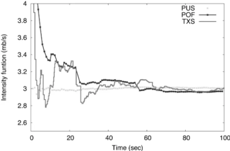
Fig. 4. Intensity functionI(t) = V (t)=tfor the three traffic traces.
and use it as an approximation to
(68) It is clear that the precision of this approximation is mainly decided by . Thus, we can pick a large enough so that its fur-ther increase would make little difference. It could sometimes be impractical to have such a long trace; however, note that even when (67) is not a good approximation of , it still rep-resents a correct result in a hypothetical periodic cross-traffic that repeats itself after every time units. This is due to the fact that in periodic cross traffic, the sample path has a lim-iting time average equal to its time average in one period.
B. Traffic Traces
We compute the probing-response curves using three dif-ferent cross-traffic types: Poisson traffic with packet sizes (in bytes) uniformly distributed in (PUS), ParetoON–OFF
traffic (POF), and a real traffic trace TXS-1148742649 (TXS) from the National Laboratory for Applied Network Research (NLANR) . Hop capacity is fixed at 10 mb/s. The cross-traffic packet size is 750 bytes for POF. The average sending rate is 500 packets per second for PUS. The mean duration of POF
ON–OFFperiods is 10 and 5 ms, respectively. The Pareto shape parameter for the duration of bothON–OFFperiods is set to 1.9. In POFON periods, the source sends CBR traffic at 750 packets per second. Given these settings, Both PUS and POF cross-traffic satisfy Assumption 1 and have a long-term arrival rate equal to 3 mb/s. To facilitate comparison, we scale the packet interarrival times in the TXS trace by a common factor so that the average traffic arrival rate within the trace duration is also 3 mb/s. We use random-number generators to produce two packet-arrival traces for PUS and POF. These traces record the time instants of all packet arrivals and their sizes within a period of 100 s.
In Fig. 4, we plot the traffic intensity function
for the three traffic traces. As shown in the figure, all traffic types have the same long-term arrival rate 3 mb/s. However, there are prominent differences in their convergence delays. Traffic trace PUS converges very fast, in 10 s, reaching within 1% of 3 mb/s. The convergence delay of POF and TXS, however, is much longer and equals about 60 s for the 1.5%-neighborhood
Fig. 5. Rate response curve for the three cross-traffic traces. (a) Probing pairs and (b) 16-packet trains (probing packet size is 750 bytes).
of 3 mb/s. Based on these cross-traffic characteristics, we choose 20 s for PUS and 60 s for POF and TXS.
In what follows, we first compute response curves for sev-eral fixed packet-train parameters. We then provide numerical results for the response deviation for a range of packet-train pa-rameters to demonstrate their quantitative relationship. For each response curve, we compute the mean output dispersion at 140 equally spaced input rates from 1 to 14 mb/s. For each input rate, we apply our offline algorithm to compute the numer-ical integration of (67) as an approximation of .
C. Results and Discussion
Fig. 5(a) shows rate response curves for the three traces when the hop is probed using 750-byte packet pairs. Notice in the figure that all three curves substantially deviate from the fluid upper bound. The curve of TXS appears lower than those of PUS and POF, indicating that TXS has the most deviation from the fluid bound of the three traces. It is also interesting to note that POF is much closer to the upper bound than PUS, which means that the former suffers lessresponse deviation than the latter. This indicates that for fixed packet-train parameters, cross traffic of more burstiness does not necessarily imply larger response deviation. We explain the reasons for this in a short while.
Fig. 5(b) shows the rate response curves for the three traces when the hop is probed using probing trains of 16 packets.
Com-Fig. 6. Log-scale NDR for the three cross-traffic traces. (a) Probing train length from 2 to 512 and (b) probing packet size from 50 bytes to 1500 bytes.
pared with the previous figure, all three response curves are closer to the fluid upper bound. However, one observation is that PUS approaches the fluid bound much quicker than the curves of the other two traces. This shows that, as the probing train length increases, the response deviation diminishes at a rate that de-pends on the burstiness of cross traffic.
Since we constantly observe that the response curves suffer the largest deviation when the input rate equals to the available bandwidth, we define a metric called NDR (normalized devia-tion ratio) to characterize the amount of deviadevia-tion in a rate re-sponse curve. Let be the output rate when the input
rate is . We define
NDR AC (69)
which is the distance of the actual curve to its upper bound di-vided by the distance to its lower bound, given that the input probing rate is equal to the available bandwidth . The NDR metric takes values in , where larger NDR values indi-cate more deviation in the response curve. We next investigate the relationship between the NDR and packet-train parameters. For all three traces, we computed the NDR using probing packet sizes between 50 and 1500 bytes with a 50-byte step and probing train lengths between 2 and 512 packets with a two-packet step. Thus, in total, we have different packet-train parameter settings for each of the three traces. For each parameter setting, we calculate the output rate in (69) using our offline algorithm.
Fig. 6(a) shows the NDR for the three traces using 750 bytes. In all cases, the NDR decreases as the probing train length increases and this relationship appears to be a power-law func-tion as confirmed by our log–log plot. Fig. 6(b) shows the NDR for a fixed train-length of 16 packets and varying probing packet size from 50 to 1500 bytes. We again observe a power-law de-crease of NDR with respect to the inde-crease in the probing packet size. Modeling the relationship between NDR and packet-train
parameters and using function NDR , where
, and are cross-traffic related parameters, we get
NDR (70)
We plot 3-D charts of NDR and their contours on log–log scale for all three traces to gain more insight into this relationship. Fig. 7 shows two of them, i.e., NDR planes for PUS and TXS. We use 3-D-fitting to find the parameters of the
Fig. 7. NDR(s; n)planes and contours for PUS and TXS. (a) PUS plane and (b) TXS plane.
TABLE I
3-D-FITTINGRESULTS FORNDR PLANES
three planes, where all least-square fitting errors are less than 5%, indicating that the power-law function (70) is a reasonable model for NDR. Curve-fitting results are given in Table I, which shows that traffic with more burstiness has smaller values of and . This explains why the response deviation in POF and TXS is harder to overcome than that in PUS.
The experimental results we obtained agree with our ana-lytical findings very well. Furthermore, they show that with fixed packet-train parameters, more cross-traffic burstiness does not necessarily imply more response deviation. However, in the former case, this deviation is more difficult to overcome by in-creasing the probing packet size or packet-train length.
To understand this phenomenon, recall that the notion of traffic burstiness in this paper relates to how fast the traffic becomes “smooth” with respect to the increase of observation intervals rather than how “smooth” the traffic appears in a given fixed observation interval. Hence, it is normal that for a given observation interval, POF has smaller variance than Poisson traffic and appears “smoother,” which leads to less response deviation when packet-trains are constructed to sample the traffic in such an observation interval. As the train length or packet size increases, the observation interval increases and Poisson traffic becomes smooth quicker than POF. Therefore, the response deviation also vanishes quicker.
Even though we do not offer a precise interpretation for the power-law relation between the NDR metric and packet-train parameters, we believe that it is related to the evolving trend of available bandwidth frequency distribution with respect to the increase of observation interval. This view is supported by the fact that the response deviation is exclusively decided by the packet-train parameters and the available bandwidth distribu-tion. This implies that there is no other factor that can decide the NDR metric.
VI. IMPLICATIONS
Among the five representative proposals TOPP, IGI/PTR, Spruce, pathload, and pathChirp, the first three directly fall under the umbrella of our work, while the last two techniques
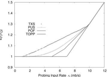
Fig. 8. TOPP-transformed rate response curves. TABLE II
TOPP RESULTS(INmb/s) USINGDEVIATIONSEGMENTS INFIG. 8 (CORRECT
VALUES:C =10 mb/s,A =7 mb/s)
have quite a few tunable parameters and their behavior is beyond the scope of this paper.
A. TOPP
Fig. 8 shows the rate response curves for the three traces when the hop is probed using 1500-byte packet-pairs (as suggested in [18]). The curves are transformed to depict the relationship between and . TOPP applies segmented linear regression on this transformed curve to obtain the hop capacity and cross-traffic intensity information. In the order of closeness to TOPP’s expected piece-wise linear curve (i.e., fluid lower bound) appear the response curves of POF, PCS, and TXS. TOPP uses the second linear segment of the measured curve assuming that it contains hop information. However, in practice, unless the deviation is very small and undetectable, the second segment may not be linear (such as in the figure) and may not coincide with the fluid bound, which may mislead TOPP into believing that the curve in the deviation range is the second linear segment of the fluid model. In Fig. 8, all deviation ranges are very clear and will be incorrectly acted upon by TOPP. Table II shows the results of a linear regression applied to deviating response curves in Fig. 8 using the basic algorithm in TOPP. As the table shows, the available bandwidth is significantlyunderestimated, espe-cially for the real traffic trace TXS. Both the hop capacity and cross-traffic intensity are significantly overestimated. Hence, to assure asymptotic accuracy, TOPP has to apply additional techniques to bypass the segment in the deviating input range.
B. PTR
PTR uses output rate at the point of transition be-tween the two linear segments in the response curve as an esti-mate of available bandwidth. As we have established, this point corresponds to the input rate at which the stochastic curve starts deviating from the fluid bound and does not usually represent
the available bandwidth of the path. Since this point is always smaller than or equal to available bandwidth, PTR is anegatively biasedavailable-bandwidth estimator in all single-hop paths.
We examine the rate response curves for the three cross-traffic traces using packet-train parameters 750 bytes and 64 packets, similar to the parameters used by PTR [6]. We find that, for PUS and POF, these parameters are sufficient for reducing the response deviation to a negligible level and producing ac-curate estimation of available bandwidth from the output rate at the deviation onset point. In both cases, the measurement bias is around 0.5 mb/s (i.e., 7% of the actual available bandwidth). For the real traffic trace TXS, the measurement bias becomes 3 mb/s, which is substantially higher and might be non-negligible for certain applications. Our analysis also leads to recommenda-tions that conflict with those stated in [6]—using larger packet size (e.g., 1500 bytes) should reduce measurement bias and not cause overestimation.
C. Spruce
Spruce uses (36) with input probing rate to estimate cross-traffic intensity. Thus, it is unbiased according to Theorem 1, regardless of the packet-train parameters and . However, by extending the analysis in this paper to multihop paths, it has been shown in [14] that cross-traffic interference from nontight hops can often cause significant amount of negative bias (often more than the actual available bandwidth) into Spruce’s esti-mator. We skip the details and refer the reader to [14] for a more thorough discussion of this issue.
VII. CONCLUDINGREMARKS
This paper focused on developing a theoretical understanding of single-hop bandwidth estimation in nonfluid cross-traffic conditions. Our main contributions include a queueing-theoretic framework of packet-train bandwidth estimation, a thorough investigation of the single-hop response deviation phenomenon, and an experimental methodology that computes the response curve with high accuracy from a given cross-traffic trace.
While we identified theresponse deviationphenomenon as one potential contributing source of measurement bias, there are certainly other important issues related to the performance of measurement techniques such as multihop effects, timing errors, and layer-2 effects [20]. Our future work involves extending this analysis to multihop paths and understanding the behavior of current measurement techniques in arbitrary network paths.
APPENDIXI PROOF OFLEMMA4
Proof: The proof is by contradiction. Suppose that does not approach 0 as . Then, there exists a
and an increasing sequence of time points with
as such that for all .
We define another sequence of time points ,
where . Then it follows
that and that for any time instant ,
, which means that interval is a hop busy pe-riod. Also, it is obvious that as , .
From Lemma 1, we can easily get the following:
(71)
Let , for sufficiently large , we have
(72) and
(73) Combining (71), (72), and (73), we get
(74) Now define a third sequence of time points such that is less than a constant for all and is a hop idle period. Then, it follows from (74) that
(75) This contradicts Assumption 1, which implies the following:
(76) Therefore, the term must approach 0 as .
APPENDIXII PROOF OFTHEOREM6
Proof: When the hop utilization process is regen-erative, the process is also regenerative with the same stopping times and regeneration cycles. Further note that the -interval available bandwidth is a time-average of the regenerative process . According to the regenera-tive central limit theorem [26, p. 124], the frequency distribution converges to a Gaussian distribution as approaches infinity, where is a constant. This implies that the mean of the Gaussian distribution remains for all , while the variance is inversely proportional to . Therefore, for sufficiently large , we have
(77) where is theGauss error function.
According to the asymptotic series of [1, pp. 297–309], we have
(78)
Combining (78) with (77), we have
(79)
where is a positive constant given below:
(80) Subtracting (79) from (28), the theorem follows.
REFERENCES
[1] M. Abramowitz and I. A. Stegun, Eds., Handbook of Mathematical Functions with Formulas, Graphs, and Mathematical Tables, ser. Ap-plied Mathematics Series, 55. Washington, DC: Nat. Bureau of Stan-dards, 1972.
[2] F. Baccelli, S. Macliiraju, D. Veitch, and J. Bolot, “The role of PASTA in network measurement,” inProc. ACM S1GCOMM, Aug. 2006, pp. 231–242.
[3] J. Bolot, “Characterizing end-to-end packet delay and loss in the in-ternet,” inProc. ACM SIGCOMM, Aug. 1993, pp. 289–298. [4] C. Dovrolis, P. Ramanathan, and D. Moore, “What do packet
disper-sion techniques measure?,” inProc. IEEE INFOCOM, Apr. 2001, pp. 905–914.
[5] G. He and J. Hou, “On exploiting long range dependence of network traffic in measuring cross traffic on an end-to-end basis,” inProc. IEEE INFOCOM, Mar. 2003, pp. 1858–1868.
[6] N. Hu and P. Steenkiste, “Evaluation and characterization of available bandwidth probing techniques,”IEEE J. Sel. Areas Commun., vol. 21, no. 6, pp. 879–894, Aug. 2003.
[7] V. Jacobson, “Congestion avoidance and control,”Proc. ACM SIG-COMM, pp. 314–329, Aug. 1988.
[8] M. Jain and C. Dovrolis, “End-to-end available bandwidth: Measure-ment methodology, dynamics, and relation with TCP throughput,”
Proc. ACM SIGCOMM, pp. 295–308, Aug. 2002.
[9] M. Jain and C. Dovrolis, “Ten fallacies and pitfalls in end-to-end available bandwidth estimation,” inProc. ACM IMC, Oct. 2004, pp. 272–277.
[10] S. Keshav, “A control-theoretic approach to flow control,”Proc. ACM SIGCOMM, pp. 3–15, Sep. 1991.
[11] K. Lai and M. Baker, “Measuring bandwidth,” inProc. IEEE IN-FOCOM, Mar. 1999, pp. 235–245.
[12] X. Liu, K. Ravindran, B. Liu, and D. Loguinov, “Single-hop probing asymptotics in available bandwidth estimation: Sample-path analysis,”
Proc. ACM IMC, pp. 300–313, Oct. 2004.
[13] X. Liu, K. Ravindran, B. Liu, and D. Loguinov, “Single-hop probing asymptotics in available bandwidth estimation: Sample-path analysis,” City University of New York, New York, Tech. Rep. TR-2004012, Aug. 2004. [Online]. Available: http://www.cs.gc.cuny.edu/tr/files/ TR-2004012.pdf
[14] X. Liu, K. Ravindran, and D. Loguinov, “Multi-hop probing asymp-totics in available bandwidth estimation: Stochastic analysis,”Proc. ACM IMC, pp. 173–186, Oct. 2005.
[15] X. Liu, K. Ravindran, and D. Loguinov, “What signals do packet-pair dispersions carry?,” inProc. IEEE INFOCOM, Mar. 2005, pp. 281–292.
[16] B. Melamed and D. Yao, “The ASTA property,” in Advances in Queueing: Theory, Methods and Open Problems, J. H. Dshalalow, Ed. Boca Raton, FL: CRC Press, 1995, pp. 195–224.
[17] B. Melander, M. Bjorkman, and P. Gunningberg, “A new end-to-end probing and analysis method for estimating bandwidth bottlenecks,” inProc. IEEE GLOBECOM Global Internet Symp., Nov. 2000, pp. 415–420.
[18] B. Melander, M. Bjorkman, and P. Gunningberg, “Regression-based available bandwidth measurements,”Proc. SPECTS, Jul. 2002. [19] E. Muhammad and S. Stidham, Sample-Path Analysis of Queueing
Sys-tems. Norwell, MA: Kluwer Academic, 1999.
[20] A. Pasztor and D. Veitch, “The packet size dependence of packet pair like methods,” inProc. IEEE/IFIP Int. Workshop on Quality of Service (IWQoS), May 2002, pp. 204–213.
[21] V. Paxson, “End-to-end Internet packet dynamics,”IEEE/ACM Trans. Netw., vol. 7, no. 3, pp. 277–292, Jun. 1999.
[22] V. Ribeiro, M. Coates, R. Riedi, S. Sarvotham, B. Hendricks, and R. Baraniuk, “Multifractal cross traffic estimation,” in Proc. ITC Specialist Seminar on IP Traffic Measurement, Monterey, CA, Sep. 2000, pp. 15-1–15-10.
[23] V. Ribeiro, R. Riedi, R. Baraniuk, J. Navratil, and L. Cottrell, “Pathchirp; Efficient available bandwidth estimation for network paths,” presented at the Passive Active Measurement Workshop, San Diego, CA, Apr. 2003.
[24] J. Strauss, D. Katabi, and F. Kaashoek, “A measurement study of avail-able bandwidth estimation tools,” inProc. ACM IMC, Oct. 2003, pp. 39–44.
[25] R. Wolff, “Poisson arrivals see time averages,”Oper. Res., vol. 30, no. 2, pp. 223–231, 1982.
[26] R. Wolff, Stochastic Modeling and the Theory of Queues. Englewood Cliffs, NJ: Prentice-Hall, 1989.
Xiliang Liureceived the B.S. (hons.) degree in com-puter science from Zhejiang University, Hangzhou, China, in 1994, the M.S. degree in information science from the Institute of Automation, Chinese Academy of Sciences, Beijing, China, in 1997, and the Ph.D. degree in computer science from the City University of New York, New York, in 2005.
He currently works for Bloomberg L.P., New York. His research interests include Internet measurement and monitoring, overlay networks, bandwidth estimation, and stochastic modeling and analysis of networked systems.
Dr. Liu has been a member of the Association for Computing Machinery (ACM) since 2002.
Kaliappa Ravindranreceived the Ph.D. degree in computer science from the University of British Co-lumbia, Vancouver, BC, Canada.
He has previously held faculty positions at the Kansas State University, Manhattan, and at the Indian Institute of Science, Bangalore. He had worked in Canadian communication industries for a short period before moving to the United States. He is currently a faculty member of computer science at the City University of New York, located in the City College campus. His research interests span the areas of service-level management of distributed networks, compositional design of network protocols, system-level support for information assurance, distributed collaborative systems, and Internet architectures. His recent industry project relationships have been with IBM, AT&T, Philips, ITT, and HP. Besides industries, some of his research has been supported by grants and contracts from federal government agencies.
Dmitri Loguinov (S’99–M’03) received the B.S. (hons.) degree in computer science from Moscow State University, Moscow, Russia, in 1995 and the Ph.D. degree in computer science from the City University of New York, New York, in 2002.
Since September 2002, he has been an Assis-tant Professor of computer science with Texas A&M University, College Station. His research interests include peer-to-peer networks, Internet video streaming, congestion control, image and video coding, and Internet traffic measurement and modeling.