DOMAIN-BASED EFFORT DISTRIBUTION MODEL FOR SOFTWARE COST ESTIMATION. Thomas Tan

(1)

DOMAIN-BASED EFFORT DISTRIBUTION MODEL FOR SOFTWARE COST ESTIMATION

by Thomas Tan

________________________________________________________________________

A Dissertation Presented to the

FACULTY OF THE USC GRADUATE SCHOOL UNIVERSITY OF SOUTHERN CALIFORNIA

In Partial Fulfillment of the Requirements for the Degree DOCTOR OF PHILOSOPHY

(COMPUTER SCIENCE) August 2012

(2)

DEDICATION

To my parents, To my family, And to my friends.

(3)

ACKNOWLEDGEMENTS

I would like to thank many of the researchers who worked alongside me through the long and painful process of data cleansing, normalization, and analyses. These individuals not only pushed me through the hardships but also enlightened me to find better solutions: Dr. Brad Clark from Software Metrics Inc, Dr. Wilson Rosa from Air Force Cost Analysis Agency, and Dr. Ray Madachy from Naval Post-graduate School.

Additionally, I like to acknowledge my colleagues from the USC Center of Systems and Software Engineering for their support and encouragement. Sue, Tip, Qi, and many others, you guys made most of my days in the research lab fun and easy and were able to pull me out of those gloomy ones.

I would also like to thank my PhD committee members who always provide insightful suggestions to guide through my research and helped me achieve my goals: Prof. Nenad Medividovic, Prof. F. Stan Settles, Prof. William GJ Halfond, and Prof. Richard Selby.

Most importantly, I would like to express my deepest gratitude to my mentor and advisor: Dr. Barry Boehm. Throughout my graduate school career at USC, Dr. Boehm has always been there guiding me to the right direction, pointing me to the right answer, and teaching me to make the right decision. His influences not only have helped me to

(4)

make through graduate school, but also will have a long lasting impact on me as a professional and scholar in the field of Software Engineering.

Last, a special thanks to the special person in my life, Sherry, who supported me with her whole heart in any way she can and provided many suggestions that proved to be more than just useful, but also brilliant.

(5)

LIST OF TABLES

Table 1: COCOMO 81 Phase Distribution of Effort: All Modes [Boehm, 1981] --- 8

Table 2: COCOMO II Waterfall Effort Distribution Percentages --- 11

Table 3: COCOMO II MBASE/RUP Effort Distribution Percentages --- 11

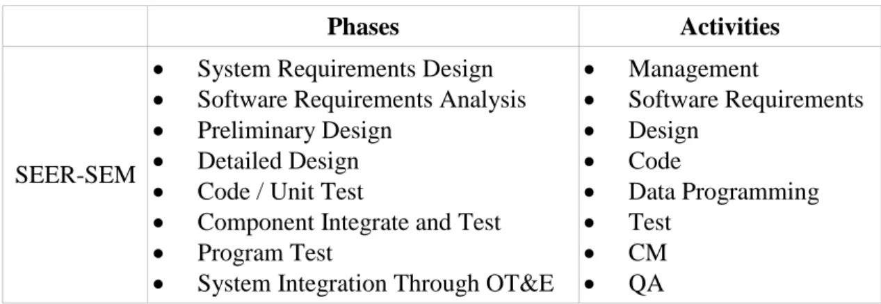
Table 4: SEER-SEM Phases and Activities --- 15

Table 5: Lifecycle Phases Supported by True S --- 16

Table 6: Mapping of SRDR Activities to COCOMO II Phases --- 23

Table 7: Comparisons of Existing Domain Taxonomies--- 26

Table 8: Productivity Types to Application Domain Mapping --- 28

Table 9: COCOMO II Waterfall Effort Distribution Percentages --- 34

Table 10: Personnel Rating Driver Values --- 36

Table 11: Data Selection and Normalization Progress --- 40

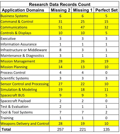
Table 12: Research Data Records Count - Application Domains --- 42

Table 13: Average Effort Percentages - Perfect Set by Application Domains --- 43

Table 14: Average Effort Percentages - Missing 2 Set by Application Domains --- 45

Table 15: ANOVA Results - Application Domains --- 47

Table 16: T-Test Results - Application Domains --- 48

Table 17: Research Data Records Count - Productivity Types --- 49

Table 18: Average Effort Percentages - Perfect Set by Productivity Types --- 50

(9)

Table 20: ANOVA Results - Productivity Types --- 52

Table 21: T-Test Results - Productivity Types --- 53

Table 22: Effort Distribution by Size Groups – Communication (Perfect) --- 54

Table 23: Effort Distribution by Size Groups - Mission Management (Perfect) --- 55

Table 24: Effort Distribution by Size Groups – Command & Control (Missing 2) - 57 Table 25: Effort Distribution by Size Groups - Sensor Control (Missing 2) --- 57

Table 26: Effort Distribution by Size Groups – RTE (Perfect) --- 60

Table 27: Effort Distribution by Size Groups - VC (Perfect) --- 60

Table 28: Effort Distribution by Size Groups - MP (Missing 2) --- 61

Table 29: Effort Distribution by Size Groups - SCI (Missing 2) --- 62

Table 30: Effort Distribution by Size Groups - SCP (Missing 2) --- 63

Table 31: Personnel Rating Analysis Results - Application Domains --- 65

Table 32: Personnel Rating Analysis Results - Productivity Types --- 67

Table 33: Effort Distribution Patterns Comparison --- 71

Table 34: Effort Distribution Patterns Comparison --- 71

Table 35: ANOVA Results Comparison --- 73

Table 36: T-Test Results Comparison --- 73

Table 37: Average Effort Percentages Table for the Domain-Based Model --- 79

Table 38: Sample Project Summary --- 83

Table 39: COCOMO II Estimation Results --- 84

Table 40: Project 49 Effort Distribution Estimate Comparison --- 85

(10)

(11)

LIST OF FIGURES

Figure 1: Cone of Uncertainty in Software Cost Estimation [Boehm, 2010] ... 3

Figure 2: RUP Hump Chart... 18

Figure 3: Research Overview ... 22

Figure 4: Example Backfilled Data Set ... 31

Figure 5: Effort Distribution Pattern - Perfect set by Application Domains ... 43

Figure 6: Effort Distribution Pattern - Missing 2 Set by Application Domains ... 45

Figure 7: Effort Distribution Pattern - Perfect set by Productivity Types ... 50

Figure 8: Effort Distribution Pattern - Missing 2 Set by Productivity Types ... 51

Figure 9: Effort Distribution by Size Groups – Communication (Perfect) ... 55

Figure 10: Effort Distribution by Size Groups - Mission Management (Perfect)... 56

Figure 11: Effort Distribution by Size Groups – Command & Control (Missing 2) 57 Figure 12: Effort Distribution by Size Groups - Sensor Control (Missing 2) ... 58

Figure 13: Effort Distribution by Size Groups – RTE (Perfect) ... 60

Figure 14: Effort Distribution by Size Groups - VC (Perfect) ... 61

Figure 15: Effort Distribution by Size Groups - MP (Missing 2) ... 62

Figure 16: Effort Distribution by Size Groups - SCI (Missing 2)... 63

Figure 17: Effort Distribution by Size Groups - SCP (Missing 2) ... 64

Figure 18: Domain-based Effort Distribution Model Structure ... 78

(12)

(13)

ABSTRACT

In software cost estimation, effort allocation is an important and usually challenging task for project management. Due to the Cone of Uncertainty effect on overall effort estimation and lack of representative effort distribution data, project managers often find it difficult to plan for staffing and other team resources. This often leads to risky decisions to assign too few or too many people to complete software lifecycle activities. As a result, projects with inaccurate resource allocation will generally experience serious schedule delay or cost overrun, which has been the outcome of 44% of the projects reported by the Standish Group [Standish, 2009].

Due to lack of data, most effort estimation models, including COCOMO II, use a one-size-fits-all distribution of effort by phase and activity. The availability of a critical mass of data from U.S. Defense Department software projects on effort distribution has enabled me to test several hypotheses that effort distributions vary by project size, personnel capability, and application domains. This dissertation will summarize the analysis approach, describe the techniques and methodologies used, and report the results. The key results were that size and personnel capability were not significant sources of effort distribution variability, but that analysis of the influence of application domain on effort distribution rejected the null hypothesis that the distributions do not vary by domains, at least for the U.S. Defense Department sector. The results were then used to

(14)

produce an enhanced version of the COCOMO II model and tool for better estimation of the effort distributions for the data-supported domains.

(15)

CHAPTER 1: INTRODUCTION

This opening chapter will reveal the motivation behind this research, state the central question and hypothesis of this dissertation, list the contributions, and introduce the organization of this dissertation.

1.1

Motivation

In most engineering projects, a good estimate does not stop when the total cost or schedule is calculated: both management and engineering team need to know the details in terms of resource allocations. In software cost estimation, the estimator must provide effort (cost) and schedule breakdowns among the primary software lifecycle activities: specification, design, implementation, testing, etc. Such effort distribution is important for many reasons, for instances:

 Before the project kick off, we need to know what types of personnel are needed at what time.

 When designing the project plan, we need to plan ahead the assignments and responsibilities with respects to team members.

 When overseeing the project’s progress, we need to make sure that the right amount of effort is being allocated to different activities.

(16)

In the COCOMO II model, supporting both Waterfall and MBASE/RUP software processes, an effort distribution percentages table is given as a guideline to help estimator in calculating the detailed effort needed for the engineering activities. However, due to the well-known Cone of Uncertainty [Boehm, 2010] effect, illustrated by Figure 1, the early stage estimate of overall project effort is considerably questionable for project management to design a reliable schedule for resource allocation.

Some progress has been made in concurrent USC-CSSE dissertation [Aroonvatanaporn, 2012] in narrowing the Cone of Uncertainty. But the uncertainty in effort distribution by activity still remains.

Due to lack of data, most effort estimation models, including COCOMO II, use a one-size-fits-all distribution of effort by phase and activity. The availability of a critical mass of data from U.S. Defense Department software projects on effort distribution has enabled me to test several hypotheses that effort distributions vary by project size, personnel capability, and application domains.

(17)

Figure 1: Cone of Uncertainty in Software Cost Estimation [Boehm, 2010]

1.2

Propositions and Hypotheses

The goal of this research work is to use information about application domain, project size, and personnel capabilities in a large software project data set to enhance the current COCOMO II effort distribution guideline in order to provide more accurate resource allocation for software projects. In order to achieve this goal, hypotheses are tested on whether different effort distribution patterns are observed from different application domains, project size, and personnel capabilities.

1.3

Contributions

(18)

1) Confirmed hypothesis that software phase effort distributions vary by domain. Rejected hypotheses that the distributions vary by project size and personnel capability.

2) Built a domain-based effort distribution model that can help to improve the accuracy of estimating resource allocation guideline for the domains, especially at the early stage of the software development lifecycle when domain knowledge may be the only available piece of information for the management team.

3) Provided a detail definition of application domains and productivity types as well as their relationship to each other. Also performed a head-to-head usability comparison to determine that domain breakdowns would be more relevant and useful as model inputs than would productivity types.

4) Provided a guideline to process and backfill missing phase distribution of effort data: use of non-negative matrix factorization.

1.4

Outline of the Dissertation

This dissertation is organized as follows: Chapter 1 introduces the research topic, its motivation, and central question and hypothesis; Chapter 2 summarizes mainstream estimation models and reviews their utilizations of domain knowledge; Chapter 3 outlines the research approach and methodologies; Chapter 4 describes the analysis results and discusses their implications and key discoveries; Chapter 5 presents the domain-based

(19)

effort distribution model with its design and implementation details; Chapter 6 concludes the dissertation with a research summary and discussion on future work.

(20)

CHAPTER 2: REVIEW OF EXISTING SOFTWARE COST

ESTIMATION MODELS AND RELATED RESEARCH STUDIES

As effort distribution is an important part of software cost estimation, many mainstream software cost estimation models provide guidelines to assist project managers in allocating resources for software projects. In section 2.1, we will review some mainstream cost estimation models and their approaches in providing effort distribution guidelines. Additionally, in section 2.2, we will examine the results of several research studies that are working toward refining the effort distribution guidelines.

2.1

Existing Software Estimation Models

2.1.1 Conventional Industry Practice

Many practitioners use a conventional industry rule-of-thumb for distributing software development efforts across a generalized software development life cycle [Borysowich, 2005]: 15 to 20 percent toward requirements, 15 to 20 percent toward analysis and design, 25 to 30 percent toward construction (coding and unit testing), 15 to 20 percent toward system-level testing and integration, and 5 to 10 percent toward transition. This approach is adapted by many mainstream software cost estimation models producing effort distribution percentage means tables through different activities or phases in the software development process.

(21)

2.1.2 COCOMO 81 Model

The COCOMO 81 Model is the first in the series of the COCOMO (COnstructive COst MOdel) models and was published by Barry Boehm [Boehm, 1981]. The original model is based on an empirical study of 63 projects at TRW Aerospace and other sources where Boehm was Director of Software Research and Technology in 1981. There are three sub models of the COCOMO 81 model: basic model, intermediate model, and detailed model. There are also three development modes: organic, semidetached, and embedded. The development mode is used to determine the development characteristics of a project and their corresponding size exponents and project constants. The basic model is quick and easy to use for a rough estimate, but it lacks accuracy. The intermediate model provides a much better overall estimate with effects from impacting cost drivers. The detailed model further enhances the accuracy of the estimate by projecting phase level with a three-level product hierarchy and adjustment of the phase-sensitive effort multipliers. The project phases supported by the COCOMO 81 model are similar to the waterfall process: including plan and requirements, product design, programming (detailed design, coding, and unit testing), and integration and test.

All three models use the effort distribution percentages table to guide resources allocation for estimators. The percentages table, as shown in Table 1, provides effort percentages for each of the development mode separated by five size groups.

(22)

Table 1: COCOMO 81 Phase Distribution of Effort: All Modes [Boehm, 1981]

Effort Distribution Size

Mode Phase Small

2 KDSI Intermediate 8 KDSI Medium 32 KDSI Large 128 KDSI Very Large 512 KDSI

Organic Plan & requirements 6 6 6 6

Product design 16 16 16 16

Programming 68 65 62 59

Detailed design 26 25 24 23 Code and unit test 42 40 38 36

Integration and test 16 19 22 25

Semi-detached

Plan & requirements 7 7 7 7 7

Product design 17 17 17 17 17

Programming 64 61 58 55 52

Detailed design 27 26 25 24 23 Code and unit test 37 35 33 31 29

Integration and test 19 22 25 28 31

Embedded Plan & requirements 8 8 8 8 8

Product design 19 19 19 19 19

Programming 60 57 54 51 48

Detailed design 28 27 26 25 24 Code and unit test 32 30 28 26 24

Integration and test 22 25 28 31 34

The general approach for determining the effort distribution is simple: the estimator can calculate the total estimate using the overall COCOMO 81 model and multiply by the given effort percentages to calculate the estimated effort for the specific phase of the given development mode and size group. This approach is the same for the basic and intermediate model but somewhat different in the detailed model where the complete step-by-step process is documented in Chapter 23 of Boehm’s publication [Boehm, 1981]. The detailed COCOMO model is based on the module-subsystem-system hierarchy and phase sensitive cost drivers, which the driver values are different by phases and/or activities. Using this model, practitioners can calculate more accurate estimates

(23)

with specific details on resource allocations. However, because this process is somewhat complicated especially considering the various cost driver values in common projects, normal practitioners often find it exhaustive to perform the detailed COCOMO estimation and would fall back on the intermediate model. Overall, use of the effort distribution percentages table is straightforward, and the approach to developing such a table sets a significant example for our research.

With regard to application types, the COCOMO 81 model eliminates the use of application types due to lack of data support and possible overlapping with other cost drivers, although Boehm suggests that application type is a useful indicator that can help to shape estimates at an early stage of a project lifecycle and a possible influential factor for effort distribution patterns. However, the notion to use the development mode is similar to using domain information: the three modes are chosen based on features that we can also use to define domain. For example, the Organic mode was applied primarily to business data processing projects. Although there are only three development modes to choose from, COCOMO 81 provides substantial assurance that domain information is carried into the calculation of both the total ownership cost and effort distribution patterns.

2.1.3 COCOMO II Model

The COCOMO II model [Boehm, 2000] inherits the approach from the COCOMO 81 model and is re-calibrated to mediate the issues in estimating costs of modern software projects such as those developed in newer lifecycle processes and capabilities. Instead of using the project modes (organic, semidetached, and embedded) to

(24)

determine the scaling exponent for the input size, the COCOMO II model suggests calculating the exponent from a set of scale factors that are identified as precedentedness, flexibility, architecture/risk resolution, team cohesion, and process maturity. These scale factors are replacements for the development modes and are meant to capture domain information in early stages: precendentedness indicates see how well we understand the system domain and flexibility to determine the domain’s conformance with requirements. The model also modifies the four sets of cost drivers to cover more aspects in modern software development practices. Equation 1 and 2 [Boehm, 2000] are the basic estimation formulas used in the COCOMO II model. The model does not take in any input of application types or environment; this information is captured by the product and platform factors (total of eight effort multipliers).

∏ (EQ. 1)

where ∑ (EQ. 2) The COCOMO II model outputs total effort, schedule, costs, and staffing as in COCOMO 81. It also continues the use of effort distribution percentages table for resource allocation guidance. The COCOMO II model replaces the original phase definition with two activity schemes: Waterfall and MBASE/RUP, which stands for Model-based Architecting and Software Engineering and was co-evolved with Rational Unified Process, or RUP [Kruchten, 2003]. The Waterfall scheme is essentially the same as defined in the COCOMO 81 model. The MBASE/RUP scheme is for the newer development lifecycle that covers the Inception, Elaboration, Construction, and Transition phases. Although the model acknowledges the variation of effort distribution

(25)

due to size, the general effort distribution percentages are not separated by size groups as they were in the COCOMO 81 model. The use of the effort distribution percentages table is similar to that in COCOMO 81; the following tables are the effort distribution percentages tables used by the COCOMO II model.

Table 2: COCOMO II Waterfall Effort Distribution Percentages Phase/Activities Effort %

Plan and Requirement 7 (2-15)

Product Design 17

Detailed Design 27-23 Code and Unit Test 37-29 Integration and Test 19-31

Transition 12 (0-20)

Table 3: COCOMO II MBASE/RUP Effort Distribution Percentages Phases (End Points) MBASE Effort % RUP Effort %

Inception (IRR to LCO) 6 (2-15) 5

Elaboration (LCO to LCA) 24 (20-28) 20 Construction (LCA to IOC) 76 (72-80) 65 Transition (IOC to PRR) 12 (0-20) 10

Totals 118 100

2.1.4 SLIM

SLIM (Software Lifecycle Model) is developed by Quantitative Software Management (QSM) based on analysis of staffing profiles and the Rayleigh distribution in software projects published by Lawrence H. Putnam in the late 1970s. SLIM can be summarized as the following equation:

[

] (EQ. 3)

(26)

In QSM’s recent release of the SLIM tool, the SLIM-Estimate [QSM] (the estimation part of the complete package) takes the primary sizing parameter of Implementation Units that can be converted from a variety of sizing metrics such as SLOC, function points, CSCI, interfaces, etc. The tool also needs to define a Productivity Index (PI) in order to produce an estimate. The Productivity Index can be derived from historical data or the QSM industry standard. It can also be adjusted by additional factors that cover software maturity to project tooling. Additional inputs such as system types, languages, personnel experiences, management constraints, etc. can also be calculated in the equation to produce the final estimate. Another important parameter for SLIM-Estimate is the Manpower Buildup Index (MBI), which is hidden from user input but derived from various user inputs on project constraints. The MBI is used to reflect the rate at which personnel are added to a project: higher rate indicates higher cost with shorter schedule, whereas lower rate results in lower cost with longer schedule. Combined with PI and size, SLIM-Estimate is able to draw the Rayleigh-Norden curve [Norden, 1958] which describes the overall delivery schedule for a project. The output of the SLIM-Estimate is usually illustrated by a distribution graph that depicts the staffing level throughout the user-defined project phases. Overall schedule, effort, and costs are produced along with a master plan that applies to both iterative and conventional development process.

SLIM-Estimate outlines the staffing resource distribution by four general phases: Concept Definitions, Requirements and Design, Construct and Test, and Perfective Maintenance. Additionally, it provides a list of WBS elements for each phase while

(27)

offering users the ability to change names, work products, and descriptions for both phases and WBS elements. Looking through SLIM-Estimate's results, we cannot find any direct connection between effort distribution and the application types input. It seems application types may be a contributor to PI or MBI for calculating the overall effort and schedule. From the overall effort and schedule, SLIM-Estimate will calculate effort distribution based on user flexibility, a parameter that SLIM-Estimate uses to choose from user-defined historical effort distribution profiles. In summary, SLIM-Estimate acknowledges that application domains or types are important inputs for its model, but does not provide specific instructions on translating application domains into estimate effort distribution patterns.

2.1.5 SEER-SEM

The System Evaluation and Estimation Resources – Software Estimation Model (SEER-SEM) is a parametric cost estimation model developed by Galorath Inc. The model is inspired by the Jensen Model [Jensen, 1983] and has evolved as one of the leading products for software cost estimation.

SEER-SEM [Galorath, 2005] accepts SLOC and function points as its primary size inputs. It incorporates a long list of environment parameters, such as complexity, personnel capabilities and experiences, development requirements, etc. Based on the inputs, the model is able to predict effort, schedule, staffing, and defects. The detail equations of the model are proprietary and we can only study the model from its inputs and outputs.

(28)

To simplify the input process, SEER-SEM allows users to choose preset scenarios that automatically populate input environment factors. The tool calls these pre-determined sets “knowledge bases,” and users can change them to fit their own needs. To determine which knowledge base to use, users need to identify the project’s platform, application types, development method, and development standard. Development methods describe the development approach such as object-oriented design, spiral, prototyping, waterfall, etc. The development standards summarize the standards for various categories such as documentation, tests, quality, etc. Platforms and application types are used to describe the product's characteristics compared with existing systems. Platforms include system built for avionics, business, ground-based, manned space, shipboard, and more. Application types cover a wide spectrum of applications from computer-aided design to command and control, and so on.

The output of the SEER-SEM tool includes overall effort, costs, and schedule. There are also a number of different reports such as estimation overview, trade-off analyses, decision support information, staffing, risks, etc. If given the work breakdown structure, SEER-SEM will also map all the estimate costs, effort, and schedule to the WBS. It is able to export out the master plan in Microsoft Project. In term of effort distribution, SEER-SEM covers eight development phases and all major lifecycle activities, as shown in Table 4. It allows full customization of these phases and activities. Effort and labor can be displayed by phases as well as by activities.

(29)

Table 4: SEER-SEM Phases and Activities

Phases Activities

SEER-SEM

 System Requirements Design  Software Requirements Analysis  Preliminary Design

 Detailed Design  Code / Unit Test

 Component Integrate and Test  Program Test

 System Integration Through OT&E

 Management  Software Requirements  Design  Code  Data Programming  Test  CM  QA

SEER-SEM uses application types as contributors to find appropriate historical profiles for setting its cost drivers and calculating estimates. The model does not provide any specific rules to link application types and effort distribution patterns.

2.1.6 True S

The Programmed Review of Information for Costing and Evaluation (PRICE) model was first developed for internal use by Frank Freiman in the 1970s at. Modified for modern software development practices in 1987, PRICE Systems released PRICE S for effort and schedule estimation for computer systems. True S [PRICE, 2005] is the current product of the PRICE S model.

True S takes a list of inputs including sizing input in SLOC, productivity and complexity factors, integration parameters, and new design/code percentages, etc. It also allows users to define application types selecting from seven categories: mathematical, string manipulation, data storage and retrieval, on-line, real-time, interactive, or operating system. There is also a platform input that describes the operating environments, structure, and reliability requirements. From the size inputs and application types, the model is able

(30)

to compute the “weight” of the software. Combined with other factors, effort in person hours or months is calculated and schedule is produced to map the nine DOD-STD-2167A phases: System Concept through Operational Test and Evaluation, detail phases shown in Table 5. TruePlanning®, the commercial suite that contains True S and the COCOMO II model, produces a staffing distribution that depicts the number of staff needed by category throughout the project lifecycle, i.e. the number of test engineers or design engineers needed as the project progresses. Additionally, True S also calculates support effort in three support phases: maintenance, enhancements, and growth.

Table 5: Lifecycle Phases Supported by True S

DoD-STD-2167A Phases Other Support Phases

True S  System Requirements  Software Requirements  Preliminary Design  Detailed Design  Code/Unit Test  Integration & Test

 Hardware/Software Integration  Field Test

 System Integration and Test  Maintenance

 Enhancement  Growth

Similar to SEER-SEM and SLIM, it is difficult to trace the connection between application type input and effort distribution guideline as there is little known about the model or how total effort is distributed to each phase. From the surface, we can only see the end results, in which a cost schedule is produced according to the engineering phases.

(31)

2.2

Research Studies on Effort Distribution Estimations

In addition to the mainstream models’ proposed effort distribution guidelines, some recent studies also focus on effort distribution patterns.

2.2.1 Studies on RUP Activity Distribution

A number of the studies are related to the Rational Unified Process (RUP) for its clear definitions in project phases and disciplines as well as straightforward guidance on effort distribution.

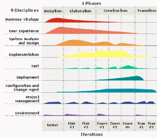
The Rational Unified Process [Kruchten, 2003] is an iterative software development process that is commonly used in modern software projects. The RUP hump chart, as shown in Figure 2, is famous for setting a general guideline of effort distribution for the RUP process. The “humps” in the chart represent the amount of effort estimated for a particular discipline over the four major life cycle phases in RUP. There are six engineering disciplines: business modeling, requirements, analysis and design, implementation, test, and deployment. There are also three supporting disciplines: configuration and change management, project management, and environment.

(32)

Figure 2: RUP Hump Chart

Over the years, there have been many attempts to validate the RUP hump chart with sample data sets. A study by Port, Chen, and Kruchten [Port, 2005] illustrates their experiment that assessed 26 classroom projects that used the MBASE/RUP process and found that their results do not follow the RUP guideline.

Similarly, Heijstek investigates Rational Unified Process effort distribution based on 21 industrial software engineering projects [Heijistek, 2008]. In his study, Heijstek compared the phase effort measured against several other studies and found that his industrial projects spent less time during elaboration and more during transition. He also produced visualization of his effort data to compare against the RUP hump chart. He observed similarities in most major disciplines, but noted discrepancies in supporting

(33)

disciplines such as configuration and change management and environment. He also extended his research in modeling the impact of effort distribution on software engineering process quality and concluded that effort distribution can serve as a predictor of system quality.

2.2.2 Studies on Effort Distribution Impact Drivers

In addition to studies on RUP, there are also works that investigate the influential factors that impact effort distribution patterns. These works also use extensive empirical analyses to back their findings.

Yang et al. [Yang, 2008] conducted a research study on 75 Chinese projects to investigate affecting factors of variant phase effort distribution. They compared the overall effort distribution percentages against the COCOMO II effort percentages and found disagreements between the two in plan/requirement and design phases. They also performed in-depth analyses on four candidate factors: development lifecycle (waterfall vs. iterative), development type (new development, re-development, or enhancement), software size (divided into 6 different size groups), and team size (four different team size groups).

For each of the candidate factors, Yang et al. compared the effort distribution between the sub-groups visually and then verified the significance of the differences using simple ANOVA tests. Their results indicate that factors such as development type, software size, and team size have visible impacts on effort distribution pattern, and they can be used as supporting drivers when making resource allocation decisions.

(34)

Kultur et al conducted a similar study with application domain as an additional factor in development type and software size [Kultur, 2009]. In their study, they filtered out 395 ISBSG data points from 4106 software projects, where each data point is given a clear application domain along with development type (new development, re-development, or enhancement) and software size. The application domains used in this research include banking, communications, electricity/gas/water, financial/property/ business services, government, insurance, manufacturing, and public administration.

The researchers compared the overall effort distribution by domains with the COCOMO II effort percentages, and suggested that some domains follow COCOMO II distribution whereas others present visible differences. Additionally, they cross-examined application domains, development types, and software size for each phase in order to uncover more detailed effort distribution patterns. They applied these distribution patterns to the sample data sets and calculated MMRE value between use of domain-specific distribution and no use of domain-domain-specific distribution. Their results indicate obvious improvements for various domains and phases and therefore call to encourage the use of domain-specific effort distribution for future analysis. However, unlike Yang’s analysis, their reports are not enclosed with detail definitions of the application domains and software process phases, which will need further investigation into the validity of their results.

(35)

CHAPTER 3: RESEARCH APPROACH AND METHODOLOGIES

This chapter documents the main approach used to achieve the research goal including descriptions of various methodologies and techniques for different analyses.

3.1

Research Overview

In order to achieve the research goal of improving the COCOMO II effort distribution guideline, I began by addressing the most complex hypothesis: the variation of effort distribution by application domain. Subsequently, I addressed the simpler hypotheses on variation by project size and personnel capability. Three smaller goals are defined to accomplish this: 1) determine the domain definitions (or domain breakdown) to be supported by the improved model; 2) find a sufficient data set; and 3) find solid evidence of different effort distribution patterns for improved effort distribution percentages for the COCOMO II model. For the smaller objectives, the following separated yet correlated studies are conducted:

1) Establish domain breakdown definitions. 2) Select and process subject data set. 3) Analyze data and build model.

Note that these studies are not necessarily done sequentially. For instance, the tasks of establishing the domain breakdown are generally done in parallel with data processing tasks so that the right domain breakdown can be generated to cover all the

(36)

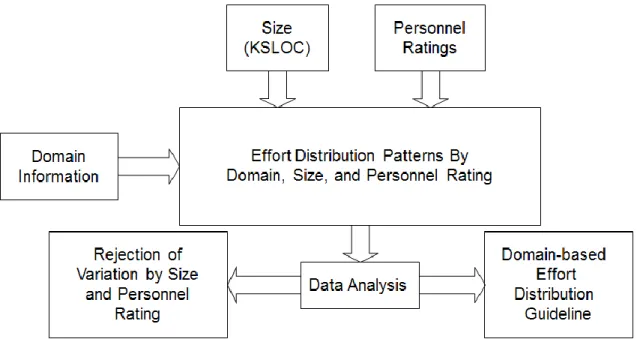
data points. Subsequently, I tested the variation hypotheses for project size and personnel capability, and found no support for the variation hypotheses. Figure 3 depicts the relationships between domains, project size, personnel capability, and the subject data set for this research. It also provides an overall guidance that lists detailed tasks for each smaller study.

Figure 3: Research Overview

3.2

Effort Distribution Definitions

In order for this research to run smoothly, a unified set of effort distribution definitions must be established before conducting any analysis. There are two sets of standard definitions that are considered for this research: development activities defined in the data dictionary from the data source [DCRC, 2005] and the COCOMO II model definitions on lifecycle activities and phases. Both sets hold their edge as the favorite for this research. Data dictionary is used by all the data points and COCOMO II model

(37)

definition is well-known and widely used by all industry leaders. Still both are not perfect on their own. Therefore, a merging effort takes place to map the overlapping activities, namely plan & requirements, architecture & design, code & unit testing, and integration & qualification tests. The result of this mapping is shown in Table 6. Using this mapping, the two sets of definitions can be connected to form a unified set that facilitates data analyses in this research. Note that because the data does not cover any transition activities, the transition phase from the COCOMO II model is excluded from this research.

Table 6: Mapping of SRDR Activities to COCOMO II Phases

COCOMO II Phase SRDR Activities

Plan and Requirement Software requirements analysis Product Design and

Detail Design Software architecture and detailed design Coding and Unit Testing Coding, unit testing

Integration and testing

Software integration and system/software integration;

Qualification/Acceptance testing

3.3

Establish Domain Breakdown

Another important set of definitions is the domain breakdown – definitions for the domains or types that are used as the input of the domain-based effort distribution model. Establishing such domain breakdown from scratch is extremely challenging. It will require years of effort summarizing distinctive features and characteristics from many different software projects with valid domain information. Then, it will need a number of Delphi discussions among various experts to establish the best definitions. A number of independent reviews will also take place in order to finalize the definitions. Any of these

(38)

tasks will take a long time to complete and the results of the new breakdown may arise from a dissertation of its own.

An alternative and rather simple approach is to research well-established domain taxonomies and use either an appropriate taxonomy or a combination of several taxonomies that have enough domain definitions to cover the research data. The following tasks outline the approach to completing the establishment of the domain breakdown:

 Select the appropriate domain taxonomies.

 Understand how these taxonomies describe the domains, i.e. the dimension that these taxonomies are using to come up with domain definitions.

 Make a master domains list and group the similar domains.  Select those that can be applied to the research data set.

Note that this part of the research is done with researchers from my sponsored program [AFCAA, 2011], with whom we are building a software cost estimation manual for the government. In this joint research, we have reviewed a long list of domain taxonomies and selected the following seven taxonomies that can cover both government and commercial projects, and are applicable to our data set:

 North American Industry Classification System (NAICS)  IBM’s Work-group Taxonomy

 Digital’s Industry and Application Taxonomy  MIL-HDBK-881A WBS Standard

(39)

 Reifer’s Application Domains

 Putnam’s Breakdown of Application Types by Productivity  McConnell’s Kinds of Software Breakdown

Among these taxonomies, NAICS [NAICS, 2007] is the official taxonomy to categorize industries based on goods-producing and service-providing functionalities of businesses. It is a rather high-level categorization, yet does provide a quality perspective on industry taxonomy. IBM [IBM, 1988] and Digital’s [Digital, 1991] taxonomies focus primarily on commercial software projects from the perspectives of both industry and system capability. Both provide comprehensive guideline in determining the software project’s domain using cross references on its industry and application characteristics. The Mil-HDBK-881A standard [DoD HDBK, 2005] is used by the US government to provide detailed WBS guideline for different military systems. The first two levels of the WBS structure provide the description of the system’s overall operating environment and high-level functionalities, thus giving us a breakdown in terms of domain knowledge. This standard is especially useful because it provides a broad view of government projects which we have not received explicitly from the previous three taxonomies. Both Putnam’s [Putnam, 1976] and McConnell’s [McConnell, 2006] application type breakdowns are based on productivity range and size divisions. This tells us that application types may contain certain software product characteristics that have direct relationships with productivity. Confirming this approach, Reifer [Reifer, 1990] also indicates the importance of productivity in relation to application domains, which he summarized from real-world data points to cover a wide range of software systems

(40)

ranging from government to commercial projects. The following table shows a comparison between our subject taxonomies.

Table 7: Comparisons of Existing Domain Taxonomies Taxonomy

Name

Number of Domains

Defined

Breakdown Rationale Considered Size Effect Considered Productivity Effect NAICS 10 industries domains. Categorizing goods-producing industries and service-providing industries.

No No

IBM 46 work groups;

8 business functions (across-industry application domains).

Use work groups as horizontal perspective and business functions as vertical perspective to pin-point a software project.

No No Digital 18 industry sectors; 18 application domains. Combines domain

characteristics with industry

definitions. No No

Reifer’s 12 application domains.

Summarized from 500 data points based on project size and productivity range.

Yes Yes

Mil-881A 8 system types. Provide WBS for each system type. Level 2 in WBS describes the application features.

No No

Putnam’s 11 application types.

Using productivity range to

categorize application types. Yes Yes McConnell’s 13 kinds of

Software.

Adopted from Putnam’s application types, refined the taxonomy with software size groups.

Yes Yes

After careful review and study of these taxonomies, we have also come to a common understanding that there are two main dimensions we can look to determine domains — platform and capability. Platform describes the operating environment in

(41)

which the software system will reside. It provides the key constraints of the software system in terms of physical space, power supplies, data storage, computing flexibility, etc. Capability outlines the intended operations of the software system and indicates the requirements of the development team in terms of domain expertise. Capability may also suggest the difficulties of the software project given nominal personnel rating of the development team.

With a prepared master list of domain categories and the notion to use both platform and capability dimensions, we put together our domain breakdown in terms of operating environment (8) and application domains (21). Each can describe a software project on its own terms. Operating environment defines the platform and product constraint of the software system whereas application domains focus on the common functionality descriptions of the software system. We can use them together or separately as they do not interfere with each other. A detailed breakdown of the operating environment and application domains is documented in Appendix A.

Although this initial version of the domain breakdown is sufficient to differentiate software project, we can do more. We have not applied productivity ratings for this breakdown. We have analyzed further breakdown using productivity rate. Upon further comparisons of these taxonomies and data analysis, a proposal was filed for a more simplified domain breakdown.

In this newer version of the domain breakdown, the 21 application domains are grouped by its productivity range. We call this new group “productivity types” or “PT”. Detailed definitions of productivity types can also be found in Appendix A. The eight

(42)

operating environments are essentially the same as the previous version but split into 10 operating environments. The following table shows a mapping between our application domains and the productivity types. Note that there are some application domains that can be mapped to more than one productivity type. This is because the application domains are covering more than one major capability that spreads across more than one productivity range.

Table 8: Productivity Types to Application Domain Mapping

Productivity Types Application Domains

Sensor Control and Signal Processing (SCP) Sensor Control and Processing

Vehicle Control (VC) Executive

Spacecraft Bus

Real Time Embedded (RTE) Communication

Controls and Displays Mission Planning

Vehicle Payload (VP) Weapons Delivery and Control

Spacecraft Payload

Mission Processing (MP) Mission Management

Mission Planning Command & Control (C&C) Command & Control

System Software (SYS) Infrastructure or Middleware Information Assurance Maintenance & Diagnostics

Telecommunications (TEL) Communication

Infrastructure or Middleware

Process Control (PC) Process Control

Scientific Systems (SCI) Scientific Systems

Simulation and Modeling

Training (TRN) Training

Test Software (TST) Test and Evaluation

Software Tools (TUL) Tools and Tool Systems

Business Systems (BIS) Business

Internet

In this research, both application domains and productivity types are candidates for support by the domain-based effort distribution model. Both breakdowns will be

(43)

thoroughly analyzed, compared, and contrasted according to the analysis procedure documented in Section 3.5.

3.4

Select and Process Subject Data

The data is primarily project data from government funded programs collected through Department of Defense’s Software Resource Data Report [DCRC, 2005]. Each data point consists of the following sets of information: a set of effort values such as person hours for requirements to qualification testing activities; a set of sizing measurements such as new size, modified size, unmodified size, etc.; and a set of project specific parameters such as maturity level, staffing, requirement volatility, etc. Additionally, each data point is attached with its own refined data dictionary. Our program sponsor, the Air Force Data Analysis Agency, sanitized the data set by removing all project identity information and helped us define the application domains and operating environment for these projects.

The original data sets are not perfect: missing data points, unrealistic data values, and ambiguous data definitions are common in our data sets. As a result, normalizing and cleansing of data points is needed for the data analyses. First, records with significant defects need to be located and eliminated from the subject data set: defects such as 1) missing important effort or size data; 2) missing data definitions on important effort or size data, i.e. no definition indicating whether size is measured in logical or physical lines of code; and 3) duplicated records. Second, abnormal and untrustworthy data patterns need to be reviewed and handled in the subject data set: patterns, which are made of huge

(44)

size with little effort or vice versa. For example, there is a record with one million lines of code, produced in 3 to 4 person months with all lines of code as new size. After removing all problematic records, two additional tasks need to be performed: 1) backfill missing effort of remaining activities and 2) test for overall normality of the data set.

There are two approaches to backfilling effort data. The first uses simple averages of the existing records to calculate the missing values. The second uses matrix factorization to approximate missing values [Au Yeung; Lee, 2001]. After a few attempts, the first approach proved to be less effective than the second and produced with large margins of errors. Therefore, the second approach, matrix factorization, is the best choice. In matrix factorization, we start with two random matrices, W and H, whose dot product equals the dimension of our data set, X0. By iteratively adjusting values of W and H, we can find the closest approximation such that W x HX, where X is an approximation of

X0. This process typically sets a maximum iteration number to be at least 5,000 to 10,000 in case W x H never reach close enough to X0. This algorithm is applied to three subsets: a subset missing 2 out of 5 activities at most; a subset missing 3 out of 5 activities, and a subset missing 4 out of 5 activities. Setting approximation exit margin to 0.001 and run for 10,000 iterations, backfilled data with very small margin of errors is produced, usually with 10% of the original (when comparing against existing data values). Figure 4 shows an example of the resulting data.

(45)

Figure 4: Example Backfilled Data Set

Notice that few records are observed with huge margin of errors. This typically results when a value for one activity is extremely small, while the values for other activities are relatively large. Although this discrepancy seems harmful to the data process results, a low number among a large collection of data points lowers the possibility of entering large error. On the positive side, this discrepancy can help us identify possible outliers in our data set if we experience situations when we need to analyze outlier effects.

The last step is to run basic normality tests on the data set. These tests are crucial because they validate the initial assumption which states that all of the data points are independent from each other and therefore normally distributed. The initial assumption is made because there is no known source information or detailed background information for all projects in the data set. We can only assume that they are not correlated in any way, and are thus independent from each other.

Since the subject data fields are effort data, it is only necessary to run the tests on this data. Both histogram and Q-Q diagrams [Blom, 1958; Upton, 1996] are produced to visualize the distribution. Several normal distribution tests such as Shapiro-Wilk test

(46)

[Shapiro, 1965], Kolmogorov-Smirnov test [Stephens, 1974], and Pearson’s Chi-square test [Pearson, 1901] are performed to check the distribution normality and to determine whether the data set is good for analysis.

In addition to checking, eliminating, and backfilling, calculating the equivalent lines of code, converting person-hours to person months, summing up the schedule in calendar months, and calculating the equivalent personnel ratings for each project are also taken place as part of the data processing.

3.5

Analyze Data and Build Model

The final piece of this research focuses on answering the central question and building an alternative model to the current COCOMO II Waterfall effort distribution guideline. There are two major steps in this part of the study: 1) calculate and analyze effort distribution patterns and 2) build and implement the model. These two steps are described in full detail in the following sub sections.

3.5.1 Analyze Effort Distribution Patterns

In studying effort distribution patterns, two rounds of analyses are conducted. In the first round, we analyze the initial version of domain breakdown with 21 application domains. In the second round, we analyze the refined version of 14 productivity types. Each round follows the same analysis steps, as described below. The results from each round will be analyzed and compared. Based on the comparison, one domain breakdown

(47)

is determined as the domain information set that will be supported by the new effort distribution model.

Effort Distribution Percentages:

From the data processing results, effort percentages by activity groups can be calculated for each project. Percentage means of each domain can also be found by grouping the records. By looking at the trend lines, simple line graph can help us visualize the distribution patterns and find interesting points. Although the plots may indicate large gaps of percentage means between domains, the evidence will not be solid enough to prove the difference significant. Statistical proofs are also needed. Single factor of variance (ANOVA) can be used for this proof. We line up all the data points in each domain and use the ANOVA test to determine whether the variance between domains is caused by mere noise or truly represents differences. The null hypothesis for this test is that all domains will have the same distribution percentage means for each activity. The alternative hypothesis is that domains have different percentage means, which is the desired result because this will prove that domains have their effect over effort distribution patterns.

Once the ANOVA tests conclude, a subsequent test must be performed to find out if the domains’ percentage means are different from COCOMO II Waterfall effort distribution guideline’s percentage means. This is important because if the domains percentage means are no different from the current COCOMO II Waterfall model, then this research will have no ground in enhancing the COCOMO II model in effort distribution. Table 9 shows the COCOMO II Waterfall effort distribution percentages.

(48)

Table 9: COCOMO II Waterfall Effort Distribution Percentages

Phase/Activity Effort %

Plan and Requirement 6.5

Product Architecture & Design 39.3

Code and Unit Testing 30.8

Integration and Qualification Testing 23.4

Note that COCOMO II model’s percentage means have been divided by 1.07 because the original COCOMO II model’s percentage means sum up to 107% of the full effort distribution.

In order to find out if there are any differences, the independent one-sample t-test [O’Connor, 2003] is used. The formula for the t-test is shown as follows:

̅ √

(EQ. 4) Statistic t in the above formula is to test the null hypothesis that sample average ̅

is equal to a specific value , where s is the standard deviation and n is the sample size. In our case, would be the COCOMO II model’s effort distribution averages and ̅ is a domain’s distribution percentage average for each activity group. The rejection of the null hypothesis in each effort activity can provide a conclusion that the domain average does not agree with the COCOMO II model’s effort distribution averages. Such an ideal result may indicate that the current COCOMO II model’s effort distribution percentages are not sufficient for accurate estimation for effort allocation and thus it is necessary to find an improvement.

In both ANOVA and t-tests, 90% significance level to accept or reject the null hypothesis is used because the data is from real world projects and the noise level is

(49)

rather high. If the tests indicate a mix between rejections and acceptances, a consensus of the results can be used to determine a final call on rejection or acceptance.

3.5.1.1Comparison of Application Domains and Productivity Types

The final step in data analysis is a comparison analysis of the results from application domains and productivity types. The purpose of this comparison is to evaluate the applicability of these domain breakdowns as the main domain definition set to be supported by the domain-based effort distribution model.

In this comparison, general effort distribution patterns are compared to find out which breakdown provides stronger trends that show more differences between domains or types. Similarly, the statistical test results are analyzed for the same reason. Lastly, the characteristics and behaviors of application domains and productivity types are analyzed to compare their identifiability, availability, and supportability.

3.5.1.2Project Size

To study project size, data points are divided into different size groups. Effort distribution patterns for each size group are produced and analyzed. The goal of this analysis is to find possible trends within a domain or type that is differentiated by project size. Since size is a direct influential driver of effort in most estimation models, a direct and simple relationship that proportionally increases or decreases project size and effort percentages is expected. Again, statistical tests are necessary if such a trend is found to prove its variance significance level.

(50)

The challenge of this analysis is the division of size groups. Some domains/types may not have enough total data points to be divided into size groups and some domains/types may not have enough data points in one or more size groups. Either case can inhibit determination of the best size driver on effort distribution patterns.

3.5.1.3Personnel Capability

For the personnel rating, the SRDR data supplies three personnel experience percentages: Highly Experienced, Nominally Experienced, and Inexperienced/Entry Level. The experience level is evaluated by the years of experience the staff has worked on software development as well as the years of experience the staff has worked within the mission discipline or project domain. Given these percentages, an overall personnel rating can be calculated using the three COCOMO II personnel rating driver values: Application Experience (APEX), Platform Experience (PLEX), and Language and Tool Experience (LTEX). The following formula is used to calculate personnel ratings for each data point. Table 10 shows the driver values of APEX, PLEX, and LTEX of different experience levels.

( ) ( )

( ) (EQ.5)

where

Table 10: Personnel Rating Driver Values

Driver Names High (~3 years) Nominal (~1 year) Low (~6 months)

APEX 0.81 1.00 1.10

PLEX 0.91 1.00 1.09

LTEX 0.91 1.00 1.09

(51)

Using the calculated personnel ratings, data points can be plotted as personnel ratings versus effort percentages for each activity group in a domain/type. Trends can be observed from these plots if increases in personnel ratings results in decreasing in effort percentages or vice versa. For simplicity, the end result for the personnel rating will be kept in linear adjustment factor (at least as close to linear as possible).

3.5.2 Build Domain-based Effort Distribution Model

From the analyses of effort distribution patterns by application domains and productivity types, project size, and personnel ratings, the variations by size and personnel ratings were negligible, and the effort distribution model was based on domain variation. A set of effort distribution percentages by application domains, and the domain definitions set to be used in the model were collected and readied to build the domain-based effort distribution model.

The key guideline for designing the model is that it has to be similar to the current COCOMO II model design. Both Waterfall and MBASE effort distribution models use average percentage tables in conjunction with size as partial influential factor. This compatibility must be established in the new model. Additionally, procedures for using the model should not be more complicated than what are currently provided by the COCOMO II model. That is, without any more instruction than to input all the COCOMO II drivers and necessary information, the model should produce the effort distribution guideline automatically as part of the COCOMO II estimates. The only additional input required may be the domain information. Comparison of the effort

(52)

distribution guideline produced by the COCOMO II Waterfall model and the new model can also be added as a new feature to make this model more useful.

When the design of the model is complete, it is important to provide an implementation instance of the model to demonstrate its features. In order to accomplish this, an instance of the COCOMO II model must be selected with source code as the implementation environment for the new model. After the new model implementation is complete, a comparison of results between COCOMO II Waterfall model and the domain-based effort distribution model must be conducted to test the new model’s performance.

(53)

CHAPTER 4: DATA ANALYSES AND RESULTS

This chapter summarizes the key data analyses and their results conducted in building the domain-based effort distribution model and testing the domain-variability hypothesis.

Section 4.1 provides an overview of the data selection and normalization results that defines the baseline data sets for the data analyses. Section 4.2 and 4.3 reports the data analyses performed on the data sets grouped by application domains and productivity types respectively. Section 4.4 reviews the analyses results and compares the pros and cons between application domains and productivity types. Finally, Section 4.5 discusses the conclusions drawn from the data analyses.

4.1

Summary of Data Selection and Normalization

Data selection and normalization are completed before most data analyses are started. A set of 1,023 project data points was collected by our data source and research sponsor, the AFCAA, and given to us for initiation of the data selection and normalization process. As discussed in Section 3.4, simple and straight forward browsing through data points helped us eliminate most defective (missing effort, size, or important data definitions such as counting method or domain information) and duplicated data points. Further analysis of abnormal data patterns also identified and removed more than

(54)

a dozen data points. A total of 530 records remains in our subject data set to begin the effort distribution analysis.

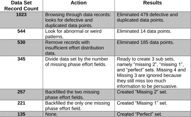
Although these 530 records are completed with total effort, size, and other important attributes, they need further processing to ensure sufficient phase effort data. Some records do not have all the phase effort distribution data that we need for the effort distribution analysis. Having eliminated those without phase effort distribution data, we are left with 345 total data points that we can work with. The table below illustrates the overall data selection and normalization progress.

Table 11: Data Selection and Normalization Progress

Data Set Record Count

Action Results

1023 Browsing through data records: looks for defective and

duplicated data points.

Eliminated 479 defective and duplicated data points. 544 Look for abnormal or weird

patterns.

Eliminated 14 data points. 530 Remove records with

insufficient effort distribution data.

Eliminated 185 data points.

345 Divide data set by the number of missing phase effort fields.

Ready to create 3 sub sets, namely “missing 2”, “missing 1”, and “perfect” sets. Missing 4 and Missing 3 are ignored because they still miss too much

information to be persuasive. 257 Backfilled the two missing

phase effort fields.

Created “Missing 2” set. 221 Backfilled the only one missing

phase effort field.

Created “Missing 1” set.

135 None. Created “Perfect” set.

“Missing 2” and “Missing 1” sets were created as comparison sets against the “Perfect” set in order to 1) increase the number of data points in the sample data set, and 2) outlook the data pattern as more data points become available in the future. The

(55)

method for backfilling is very effective in predicting continuous and correlated data patterns such as the effort distri