University of Cape Town
Melusi Manqoba Mavuso
A dissertation submitted to the Department of Actuarial Science, Faculty of Commerce, at the University of the Cape Town, in partial fulfilment of the
requirements for the degree of Master of Philosophy.
October 10, 2014
Master of Philosophy specializing in Mathematical Finance, University of the Cape Town,
The copyright of this thesis vests in the author. No
quotation from it or information derived from it is to be
published without full acknowledgement of the source.
The thesis is to be used for private study or
non-commercial research purposes only.
Published by the University of Cape Town (UCT) in terms
of the non-exclusive license granted to UCT by the author.
I declare that this dissertation is my own, unaided work. It is being submitted for the Degree of Master of Philosophy in the University of the Cape Town. It has not been submitted before for any degree or examination in any other University.
April 8, 2015
Consider a market consisting of two correlated assets: one liquidly traded asset and one illiquid asset that can only be traded at time 0. For a European derivative written on the illiquid asset, we find a hedging strategy consisting of a constant (time 0) holding in the illiquid asset and dynamic trading strategies in the liquid asset and a riskless bank account that minimizes the expected square replication error at maturity. This mean–variance optimal strategy is first found when the liquidly traded asset is a local martingale under the real world probability measure through an application of the Kunita–Watanabe projection onto the space of attainable claims. The result is then extended to the case where the liquidly traded asset is a continuous square integrable semimartingale, and we again use the Kunita–Watanabe decomposition, now under the variance optimal martingale measure, to find the mean–variance optimal strategy in feedback form. In an example, we consider the case where the two assets are driven by correlated Brownian motions and the derivative is a call option on the illiquid asset. We use this example to compare the terminal hedging profit and loss of the optimal strategy to a corresponding strategy that does not use the static hedge in the illiquid asset and conclude that the use of the static hedge reduces the expected square replication error significantly (by up to 90% in some cases). We also give closed form expressions for the expected square replication error in terms of integrals of well–known special functions.
First, I would like to acknowledge the help and guidance from my supervisor A/Prof. Tom McWalter. Your suggestions were very helpful!
I would also like to thank my co-supervisors from Old Mutual, Mr Dylan Flint and Dr. Marc-hand van Rooyen, for structuring a problem that has enabled me to learn so much just from trying to solve it.
I would like to thank Mr Ralph Rudd for taking his time to proofread my dissertation and help me correct some errors.
I would also like to thank the UCT department of statistical sciences for the warm treat-ment throughout the year.
Finally, I would like to thank Mr Armin van Buuren for keeping me in ‘a state of trance’ during the long nights of typing this dissertation.
I dedicate this work to my friends, colleagues and everyone who was getting tired of hear-ing the phrase “my dissertation is essentially completed”. Thank you for askhear-ing, it kept me going!
Thank you mom and grandma for the support you’ve given me throughout my academic career.
1. Introduction . . . 1
1.1 Problem Formulation . . . 1
1.2 The Structure of the Dissertation . . . 3
2. Preliminaries . . . 5
2.1 Hilbert Spaces . . . 5
2.1.1 Elementary Results and Definitions . . . 5
2.1.2 Direct Sums, Orthogonality and Projections . . . 7
2.2 Stochastic Processes . . . 8
2.2.1 Stochastic Processes . . . 8
2.2.2 Square Integrable Martingales . . . 12
2.3 Continuous Trading . . . 14
2.3.1 Theory of Continuous Trading . . . 14
2.3.2 A Complete Market Model . . . 17
3. Hedging in an Illiquid Market: The Martingale Case . . . 19
3.1 Incomplete Markets: a Result by F¨ollmer and Sondermann . . . 19
3.1.1 Mean–Variance Hedging . . . 21
3.2 Application to Hedging in an Illiquid Market . . . 23
3.3 Finding The Best Hedge: General Payoff . . . 26
3.4 Finding The Best Hedge: Call Option . . . 29
4. Hedging in an Illiquid Market: The Semimartingale Case . . . 33
4.1 Mean–Variance Hedging . . . 33
4.2 Application to Hedging in an Illiquid Market . . . 37
4.3 The Brownian Motion Model . . . 40
4.3.1 General Payoff . . . 41
4.3.2 Call Option . . . 44
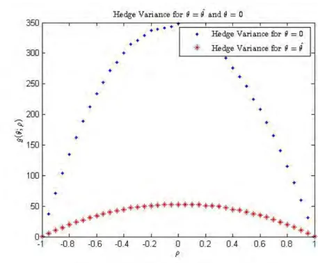
4.3.3 Some Numerical Results . . . 46
5. Conclusion . . . 51
Bibliography . . . 52
4.1 Expected square replication error from simulation . . . 47
4.2 Exact expected square replication error . . . 47
4.3 Expected square replication error as a function of correlation . . . 48
4.4 Histogram of terminal hedging error with static hedge . . . 49
4.5 Histogram of terminal hedging error without static hedge . . . 49
4.6 Two sample paths of stock holdings . . . 50
Introduction
One of the recent major breakthroughs in the mathematics of finance is the idea that one can (in theory) eliminate the risk carried in writing an option by trading in the underlying security and a riskless asset. This idea of replication was first presented by Black and Scholes (1973) and Merton (1973) and was further studied by Harrison and Kreps (1979), Kreps (1981), Harrison and Pliska (1981) and Harrison and Pliska (1983) in their seminal papers of the late 70s and early 80s.
However, in order for such a perfect replication to be possible, many assumptions are made. Some of these include continuous trading, absence of transaction costs and unlimited short selling. Relaxing these assumptions has been the subject of enormous research in the last three decades and substantial progress has been made. This dissertation focuses on solving a problem where continuous trading is restricted to one of two assets.
1.1
Problem Formulation
Consider a company (e.g. a bank or insurance company) that has an obligation to make a payment at some future time T > 0 represented by the random variable H. Such a random payment could, for instance, be an option on a share or an annuity to policyholders. Ideally, the company would want to construct a portfolio of assets to trade that will have the same value as H at time T, under all circumstances. If this is not possible, the requirement might be relaxed to finding a portfolio of assets whose value is as ‘close as possible’ to H at time T.
To put this into perspective, assume thatH is an option written on a stock whose (discounted) price process is denoted by ¯U. Under certain models for ¯U (and integrability conditions onH), the theory of Black and Scholes (1973) shows that it is possible to construct a dynamic trading strategy in ¯U and the riskless bank account that will replicateH under all circumstances. This replication process makes use of all the ‘frictionless’ market assumptions of Harrison and Pliska (1983) and our aim is to relax the assumption of continuous trading in ¯U.
We consider the case when the asset ¯U is not liquid and continuous trading in ¯U is thus not possible. We further assume that, together with a riskless bank account, there is another asset X that is correlated to ¯U, which can be traded continuously without any restrictions (so that all the assumptions of Black and Scholes (1973) hold for trading the asset X). The question arises: how does one utilize the ability to trade partly in the illiquid asset ¯U and the liquid asset X together with the riskless asset to reduce the risk of writing (or even holding) the derivativeH? Such a hedging strategy will generally not replicateH, except in trivial cases such as whenX and ¯U are perfectly correlated. So, in general, we can only hope to make the portfolio value as ‘close as possible’ to H at time T.
in which the asset ¯U may be illiquid. Also, we need to make precise what it means to make the portfolio value as ‘close as possible’ to H at timeT.
One interpretation of ¯U being illiquid might be that trading in ¯U is not possible at all times. In that case we have to construct the ‘best’ strategy using only asset X (and the riskless bank account). This problem has been studied extensively in the literature under the topic of Hedging in an Incomplete Market. Some references in that direction include Schweizer (1991), Duffie and Richardson (1991), Schweizer (1992), Davis (2006) and Monoyios (2004). A specific example of thishedging of basis risk problem is also considered by McWalter (2007) and Hul-ley and McWalter (2008) in the case whenX and ¯U are correlated geometric Brownian motions.
The aim of this dissertation is to consider a slight change to the above by assuming that the asset ¯U can be traded only once — at the inception of the contract. Thus, any ‘admissible’ trading strategy will consist of a static hedge in ¯U and a dynamic hedge in both X and the bank account.
As mentioned before, the new trading strategy described above will generally not replicate the payoff H. We therefore need a criteria by which to choose the ‘best’ trading strategy. An obvious way of doing this is to define a utility function and then choose a strategy that maximizes the expected utility. This type of reasoning has been followed by (among others) Davis (2006).
In this dissertation we choose tominimize a certain kind of quadratic utility functional. To be more precise, if VT is the value of a trading strategy at time T, we will choose a strategy that
minimizes the expected square replication error:
E((VT −H)2)
over all admissible trading strategies. This is known as mean–variance hedging and was first considered by F¨ollmer and Sondermann (1986) in the case whenXis a martingale under the real world probability measureP. It was later generalized by (among others) Duffie and Richardson (1991) in the Brownian motion setting and by Schweizer (1988), F¨ollmer and Schweizer (1991), Schweizer (1991), Schweizer (1992), Rheinlander and Schweizer (1997) and Gouri´eroux et al. (1998) to the case whenX is a semimartingale underP. This criterion is also used by McWalter (2007) and Hulley and McWalter (2008) in the context of a two dimensional Brownian motion model for X and ¯U, which provided us with the initial motivation to extend their results.
To formulate the problem mathematically, we want to find a constant holding ˆθ in ¯U, a dynamic trading strategy ˆϕ ={ϕˆt : 0 ≤ t ≤ T} in X and a dynamic strategy ˆη = {ηˆt : 0 ≤t ≤ T} in
the bank accountB that will minimize
E((VT −H)2) =E((θU¯T +ϕTXT +ηTBT −H)2)
over all such trading strategies (θ, ϕ, η). Without loss of generality, we will work with discounted assets and setB ≡1. The problem is then to minimize
E((VT −H)2) = E((θU¯T +ϕTXT +ηT −H)2)
over all such trading strategies (θ, ϕ, η). Also, confining ourselves to self–financing strategies, the problem simplifies to minimizing
E v0+ Z T 0 ϕtdXt+θU¯T −H 2!
over all strategies (θ, ϕ, v0), where v0 is the initial capital required for the dynamic strategy
inX and the bank account. The dependence onηis dropped due to the self–financing condition.
If H ∈ L2 and V
T ∈ L2 for each admissible strategy (θ, ϕ, v0), then this problem is
equiva-lent to finding anL2 projection ofH onto the space of attainable claims; therefore if this space is closed in L2, a unique solution will exist by the Projection Theorem. Whether or not this
space is closed turns out to be very different when X is a local martingale to when X is only a semimartingale underP. The local martingale case is easy and transparent — in that case the space of attainable claims is closed inL2 by the Itˆo isometry. It is for this reason that we first
consider the martingale case.
In both cases, we use ideas from the solution of hedging in an incomplete market with no trading constraints. The solution to this problem was found by F¨ollmer and Sondermann (1986) when X is a square integrable martingale and later generalized by Schweizer (2001) to whenXis a local martingale. For the semimartingale case, more assumptions onX are required for the space of attainable claims to be closed. However in both cases, the Kunita–Watanabe decomposition proves to be vital in solving the problem. When X is a local martingale, this decomposition is used to find a projection onto the space of stochastic integrals with respect to X, while after a change of measure to the variance–optimal martingale measure, the same projection is used when X is only a semimartingale.
In general, even the optimal strategy will not necessarily replicate the payoff exactly. Another aim of this dissertation is to derive closed form expressions for the expected square replication error. This quantity is normally found using simulations in the literature (e.g. see Heath et al. (2001b) and Hulley and McWalter (2008)), but we manage to write integral expressions of this quantity in terms of well–known special functions for Brownian motion stocks and when H is a call option on ¯U.
1.2
The Structure of the Dissertation
The dissertation is divided into five chapters. The second chapter gives a summary of the main definitions, notation and preliminary results that we use throughout the dissertation. This is done in a quick way and proofs are not given. The reader is referred to relevant sources in the literature. This chapter can be skimmed through by the well informed reader.
In Chapter 3 we solve the problem stated above in the special case when the liquidly traded assetXis a local martingale under P. We start by discussing general mean–variance hedging in an incomplete market whenX is a local martingale and make a presentation similar to F¨ollmer and Sondermann (1986) and Schweizer (2001). We then use a similar argument to solve the illiquid market hedging problem. The solution turns out to be a simple application of the projection theorem to an appropriate closed subspace. We also consider an example when X
and ¯U are driven by correlated Brownian motion processes andH is a call option on ¯U. In this example we derive closed–form expressions for the expected square replication error in terms of well–known special functions.
The main purpose of Chapter 4 is to extend the results of Chapter 3 to the case when X
is a continuous semimartingale. This chapter is very similar in style to Chapter 3. We again start off by discussing mean–variance hedging in an incomplete market whenXis a semimartin-gale. We follow presentations by Gouri´eroux et al.(1998) and Heathet al. (2001a) and observe that different assumptions onX guarantee the closedness of the space of attainable claims. We
then apply these results to find a solution to our problem by first fixing the constant holding in ¯
U to be θ, treating the problem as an incomplete market hedging problem of a modified claim and then finding the optimal value of θ. These results are then applied to a two–dimensional geometric Brownian motion model for X and ¯U similar to the one used in Chapter 3. Closed– form expressions for the expected square replication error are found and we also provide some numerical results for specific model parameters.
The last chapter concludes by giving some possible extensions of these results and discussing some comparisons. This dissertation should be accessible to a graduate student with a back-ground in stochastic calculus and elementary mathematical finance.
Preliminaries
This chapter presents definitions and results that will be used throughout the dissertation. It is assumed that the reader is familiar with these concepts and no proofs will be provided; instead we make reference to relevant papers and textbooks.
2.1
Hilbert Spaces
In this section we quickly recall some important results and definitions in Hilbert spaces that will be used throughout. We simply state the main results without proof and refer the reader to any standard textbook on analysis for any proofs. Some examples include Brezis (2011), Zeidler (1995) and Conway (1990). We assume that the reader is familiar with basic analysis in metric and normed spaces. We also assume that all vector spaces considered are over the field Rof real numbers. Both the zero vector and the number zero are denoted by 0.
2.1.1
Elementary Results and Definitions
Definition 2.1.1. Let V be a vector space. An inner product on V is a function (·,·) :
V ×V −→R such that for every u, v, w ∈V and α ∈R, 1. (u, u)≥0 and (u, u) = 0 if and only if u= 0 2. (u, v) = (v, u)
3. (αu, v) =α(u, v)
4. (u+v, w) = (u, w) + (v, w).
The pair (V,(·,·)) is called an inner product space or pre-Hilbert space.
We will often refer to V (on its own) as an inner product space if the inner product is clear from the context.
Theorem 2.1.1. If (V,(·,·)) is an inner product space, then for every u, v ∈V
|(u, v)|2≤(u, u) (v, v). (2.1)
Inequality (2.1) is known as the Cauchy–Schwartz inequality and is used to show the fol-lowing:
Theorem 2.1.2. If (V,(·,·))is an inner product space, then the function ||·||:V −→R defined by
||v||:=p(v, v) for every v ∈V (2.2) is a norm on V. This makes (V,||·||) a normed space and a metric space under the metric d
defined by
A sequence (vn) in a normed spaceV is a functionv :N+−→V. We say that (vn) converges
tov ∈V if for every >0 there existsN ∈N+ such that for everyn≥N, we have||v
n−v||< .
We will write vn −→v or lim
n→∞vn=v to say that (vn) converges to v.
Definition 2.1.2. A sequence (vn) in a normed space V is a Cauchy sequence if for every
>0 there exist N ∈N+ such that for every n, m∈
N+, if n, m≥N, then ||vn−vm||< .
It is clear that every convergent sequence is Cauchy. Indeed, assume that (vn) converges to
v and let > 0. Choose N ∈ N+ such that if n ≥ N, then ||v
n−v||< 2. Now if n, m ≥ N,
then||vn−vm||=||vn−v+v−vm||≤ ||vn−v||+||vm−v||< 2+2 =. The converse, however,
does not hold in general.
Definition 2.1.3. An inner product space V is complete if for every Cauchy sequence (vn)
in V, there exists v ∈ V such that vn −→ v; i.e. V is complete if every Cauchy sequence in
V converges to an element of V. A subset U of V is complete if every Cauchy sequence in U
converges to an element of U.
A complete inner product space is called a Hilbert space.
Theorem 2.1.3. If V is a finite dimensional inner product space, then V is a Hilbert space; i.e. every finite dimensional inner product space is complete.
An analogous result is also true for normed spaces in general; complete normed spaces are calledBanach spaces.
Definition 2.1.4. A subset U of a normed space V is closed in V (or simply closed if the normed space is clear from the context) if every convergent sequence inU has a limit in U; i.e.
U is closed if it satisfies the condition that if (vn) is a sequence with vn ∈U for every n ∈N+
and vn −→v ∈V, then v ∈U.
Theorem 2.1.4. If V is a normed space and U ⊆ V is a finite dimensional subspace of V, then U is closed; i.e. every finite dimensional subspace of a normed space V is closed.
Theorem 2.1.5. If V is a Hilbert space, then U ⊆V is closed if and only if U is complete. LetV and W be vector spaces. Recall that a map T :V −→W is linear if
T(αu+βv) = αT(u) +βT(v) for everyu, v ∈V and α, β ∈R.
Definition 2.1.5. Let (V,||·||V) and(W,||·||W) be normed spaces and T :V −→W be a linear
map.
1. We call T an isomorphism if T is one to one and onto; i.e. bijective. 2. We call T an isometry if
||T(v)||W=||v||V for every v ∈V.
We say that T is an isometric isomorphism if T is both an isomorphism and an isometry. If there exist an isometric isomorphism T : V −→ W, then the normed spaces V and W
are said to be isometrically isomorphic. Normed spaces that are isometrically isomorphic are essentially the same as normed spaces.
Theorem 2.1.6. Let V and W be inner product spaces (and therefore normed spaces) that are isometrically isomorphic. IfV is a Hilbert space, then so is W and conversely.
2.1.2
Direct Sums, Orthogonality and Projections
IfV is a vector space and U1, U2 are subsets of V, then we define U1+U2 as
U1+U2 :={u1+u2 :u1 ∈U1, u2 ∈U2}.
Definition 2.1.6. Let V be a vector space, U1 and U2 be subspaces (non-empty, closed under
vector addition and scalar multiplication) of V. Then
1. V is a sumof U1 and U2 (written as V =U1+U2) if for every v ∈V there existu1 ∈U1
and u2 ∈U2 such that v =u1+u2.
2. V is a direct sum of U1 and U2 (written as V =U1⊕U2) if for every v ∈V there exist
unique u1 ∈U1 and u2 ∈U2 such that v =u1+u2.
Theorem 2.1.7. Let V be a vector space and U1 and U2 be subspaces of V. The following are
equivalent:
1. V =U1⊕U2
2. V =U1+U2 and U1∩U2 ={0}.
One question that we need to answer for later chapters is the following: if U1 and U2 are
closed subspaces of a Hilbert space V, is U1+U2 closed? It turns out that this is not true in
general unless at least one of them is finite dimensional.
Theorem 2.1.8. IfU1 andU2 are closed subspaces of a Hilbert spaceV andU1 (orU2) is finite
dimensional, then U1+U2 is closed.
Definition 2.1.7. Let V be an inner product space. We say that u, v ∈ V are orthogonal
(written asu⊥v) if (u, v) = 0. If U ⊆V we define the orthogonal compliment of U by
U⊥ :={v ∈V : (u, v) = 0 for all u∈U}={v ∈V :v ⊥u for all u∈U}.
Theorem 2.1.9. Let U be a subset of an inner product spaceV. Then U⊥ is a closed subspace of V.
We are now in a position to solve the following problem: Given a Hilbert space V, a subset
U of V and an element v ∈V, find u∈U that best approximates v inU. That is, we want to find u∈U such that
||v−u||= inf
w∈U||v−w||.
Such an element u, if it exists, is called the projection of v onto U. This problem is more interesting of course when v ∈ V\U, since we may choose u = v if v ∈ U. Here u is the best estimator of v in U, where ‘best’ is measured in terms of minimizing the norm. The question of existence (and uniqueness) of such a best estimator for an arbitrary v ∈ V\U depends on both the topology and geometry ofU.
If V is a vector space, then U ⊆ V is convex if for every u, v ∈ U and λ ∈ [0,1], we have
λu+ (1−λ)v ∈ U. Subspaces provide good examples of convex subsets since they are closed addition and scalar multiplication.
Theorem 2.1.10. Let V be a Hilbert space and U ⊆ V be a non–empty closed and convex subset of V. Then for every v ∈V, there exist a unique u∈U such that
||v−u||= inf
w∈U||v−w||.
Furthermore, u is the unique element of U that satisfies the following (variational) inequality (v−u, w−u)≤0 for all w∈U.
The above theorem gives a sufficient condition for a projection on a subset U of V to exist for every element. An important special case is when U is actually a closed subspace of a V. In that case we get the celebrated projection theorem.
Theorem 2.1.11. Let U be a closed subspace of a Hilbert space V.
1. For every v ∈ V, there exists a unique projection u of v onto U. Furthermore, u is such that v−u∈U⊥ (i.e. (v−u, w) = 0 for every w∈U).
2. V =U ⊕U⊥; i.e. for every v ∈V, there exist unique elements u∈U and u⊥ ∈U⊥ such that v =u+u⊥.
The projection theorem tells us that if U is a closed subspace of a Hilbert space V, then eachv ∈V can be associated with a unique PU(v) := u∈U such that
||v −PU(v)||= inf
w∈U||v−w||.
This defines a map PU :V −→ U ⊆V. This map is called the orthogonal projection onto
U and it has the following properties:
1. PU is linear; i.e. PU(αv1+βv2) =αPU(v1) +βPU(v2) for every v1, v2 ∈V and α, β ∈R
2. PU is continuous; i.e. If vn−→v in V, then PU(vn)−→P(v)
3. PU is non-expansive; i.e. ||PU(v)||≤ ||v||for every v ∈V
4. PU is idempotent; i.e. PU(PU(v)) = PU(v) for everyv ∈V.
Theorthogonal decomposition ofv ∈V asv =PU(v) + (v−PU(v), wherePU(v) andv−PU(v)
are orthogonal, is at the heart of this dissertation.
2.2
Stochastic Processes
Much of what we will be doing deals with stochastic processes. In this short section we give brief definitions and important results in stochastic processes and stochastic calculus. The main references used are Protter (2004), Rheinlander (2011), Karatzas and Shreve (1991), Jacod and Shiryaev (2003) and Durrett (1996). We again assume that the reader is familiar with all the theory of stochastic processes, including probability and measure theory, together with modes of convergence of sequences of random variables.
2.2.1
Stochastic Processes
Throughout we fix a probability space (Ω,F,P). For 1≤p <∞we denote byLp(
P) the vector
space of equivalence classes of random variablesX with E(|X|p)<∞. With the understanding
that we identify random variables that agree almost surely (a.s.), we will simply think ofLp(P) as a space of random variables. We will also writeLp if the measure
Pis clear from the context.
Theorem 2.2.1. For 1 ≤ p < ∞, the space Lp is a Banach space with norm ||X|| Lp= (E(|X|p))1/p
and L2 is a Hilbert space with inner product defined by (X, Y) :=E(XY) for every X, Y ∈L2.
Astochastic processX on (Ω,F,P) is an indexed collection of random variables. We will deal only with stochastic processes that are indexed by time in some intervalI ⊆R+ := [0,∞).
For now we set I =R+. Then
X :={Xt:t ∈R+},
where eachXtis a random variable. If we fix ω ∈Ω, then{Xt(ω) :t∈R+}is called a sample
path of X. Two stochastic processes X and Y are indistinguishable if
P ω ∈Ω :Xt(ω) =Yt(ω) t∈R+ = 1.
We will use this to define equality of stochastic processes and write X = Y if and only if X
and Y are indistinguishable. A filtration F = {Ft : t ∈ R+} on (Ω,F,P) is an increasing
collection of sub–sigma algebras of F. We will assume that F always satisfies the following
usual conditions of continuity and completeness:
1. F0 contains all the P–null sets of F (this is called completeness)
2. F is right continuous in the sense that for every t ∈R+,
Ft+ :=
\
s>t
Fs =Ft.
For all our applications it will be convenient to further assume that F0 is trivial in the sense
that it contains only events of probability zero or one. We then call (Ω,F,F,P) a filtered probability space. X is said to be adapted to F (or simply adapted, if F is known) if Xt
is Ft–measurable for each t. All processes we deal with will be assumed to be adapted
un-less explicitly stated otherwise. We denote by FX the filtration generated by X. That is
FX =σ(X).
The process X is said to be continuous if almost all the sample paths of X are a contin-uous function of t ∈ R+ and X is c`adl`ag (resp. c`agl`ad) if X is right continuous with finite
left limits (resp. left continuous with finite right limits). For a c`adl`ag process X, we will define the processX−:={Xt− :t∈R+}by
Xt− := lim
s→t−Xs
and the jump process∆X =X −X− with ∆X0 = 0. We note that if X is continuous then
∆X ≡0.
A random variableτ : Ω−→[0,∞] is a stopping timeif {τ ≤t} ∈ Ft for every t ∈R+. If τ
is a stopping time, then the process Xτ defined by settingXτ
t :=Xτ∧t=Xmin(τ,t) is called the
stopped process. If E is a set of stochastic processes, X is said to be locally in E if there exist an increasing sequence of stopping times (τn) such that τ → ∞ P–a.s. and Xτn ∈ E for
every positive integer n. The sequence (τn) is called a localizing sequence for X and the
set of all processes that are locally in E is denoted by Eloc. We say that E is stable under
stopping if X ∈ E ⇒Xτ ∈ E for any stopping time τ.
Let L be the collection of all adapted c`agl`ad (left continuous with right limits) processes on (Ω,F,F,P). The sigma field generated by elements ofLis called thepredictable sigma field. This is a sigma field on Ω×R+ and is denoted by P. That is
P :=σ(L).
It is shown in Revuz and Yor (1999) that if F satisfies the usual conditions (which is what we will always assume), then P is also generated by the continuous adapted processes. A process
X is said to be predictable if the map (ω, t)7→Xt(ω) from Ω×R+ toR is P–measurable.
Now let t ∈ R+ and consider a partition of [0, t]: πk
t := {t0, t1, . . . , tk} , where k is a
posi-tive integer and 0 = t0 ≤ t1 ≤ t2 ≤ . . . ≤ tk = t. We define the total variation process
V(1)(X) ofX as (supremum over all partitions πtk of [0, t])
Vt(1)(X) := sup πk t k X i=1 |Xti−Xti−1| ! .
IfVt(1)(X)<∞ a.s. for every t, we say X is of finite variation. We will also write the total variation ofX as
Vt(1)(X) :=
Z t
0
|dX|s.
IfX is of finite variation, we can define the integral of a locally bounded process ϕwith respect toX as a path-wise Lebesgue–Stieltjes integral. We denote this integral by
(ϕ·X)t:= Z t 0 ϕsdXs, so that (ϕ·X)t(ω) := Z t 0 ϕs(ω)dXs(ω) for every ω∈Ω.
Definition 2.2.1. A process M is a martingale with respect to F if 1. M is adapted to F
2. E(|Mt|)<∞ for every t∈R+; i.e. Mt is integrable for every t∈R+
3. E(Mt|Fs) = Ms for s < t.
We say that M is a submartingale (resp. supermartingale) if it satisfies 1 and 2 and
E(Mt|Fs)≥Ms (resp. E(Mt|Fs)≤Ms) for s < t.
M is alocal martingale if there exist an increasing sequence of stopping times (τn) with
τn → ∞such that the stopped processMτn ={Mτn∧t :t∈R
+}is a martingale for eachn∈ N+.
Local martingales are generally not of finite variation, thus the integral with respect to a local martingale cannot be defined as a path–wise Lebesgue–Stieltjes integral. The construction of this stochastic integral is beyond the scope of this presentation and is discussed by many textbooks (see for example Protter (2004) or Jacod and Shiryaev (2003)). We will not go through this construction but simply mention that this ‘stochastic integral’ with respect to a local martingaleM is well defined for predictable processes ϕand is also a local martingale. It will also be denoted by
(ϕ·M)s :=
Z t
0
ϕsdMs.
We define asemimartingale to be a process X that can be written as
X =X0 +M +A,
whereX0 is finite,M is a local martingale andAis an adapted process of finite variation, both
null at 0 (i.e. their values are zero att= 0). IfA is also predictable, thenX is called aspecial semimartingale. We will denote the vector space of semimartingales by S and the space of
special semimartingales bySp. The stochastic integral of a locally bounded predictable process
ϕwith respect to a semimartingale X is defined as
(ϕ·X)t:= (ϕ·M)t+ (ϕ·A)t i.e. Z t 0 ϕsdXs:= Z t 0 ϕsdMs+ Z t 0 ϕsdAs. (2.3)
We will sometimes write (2.3) in differential notation as
d(ϕ·X)t =ϕtdXt=ϕtdMt+ϕtdAt.
We sayϕis X–integrableif (ϕ·X) is finite. The space of X–integrable processes is denoted byL(X). For ϕ∈ L(X), the process (ϕ·X) is also a semimartingale. The stochastic integral can also be generalized tod–dimensional processes. For further details, see Protter (2004).
IfX and Y are martingales, we define the cross variationprocess of X and Y as
hX, Yit := sup πk t k X i=1 Xti −Xti−1 Yti −Yti−1 ! ,
where the supremum is taken over all partitions πk
t of [0, t]. We call hXi = hX, Xi the
quadratic variation of X. We will also define the cross variation and quadratic variation this way whenX and Y are continuous semimartingales.
Theorem 2.2.2. Let X and Y be continuous semimartingales and ϕ ∈ L(X), η ∈ L(Y) be continuous. Then Z t 0 ϕsdXs, Z t 0 ηsdYs = Z t 0 ϕsηsdhX, Yis.
In particular, this result tells us that
Z t 0 ϕsdXs = Z t 0 ϕ2sdhXis.
We also define thestochastic exponentialof a continuous semimartingale X as
E(X)t := exp Xt− 1 2hXit .
We end this section with a very useful formula for continuous semimartingales. The following is Theorem 3.3 of Revuz and Yor (1999).
Theorem 2.2.3 (Itˆo’s formula). Let X = (X1, . . . , Xd) be a d–dimensional continuous semi-martingale and f ∈C2(
Rd,R). Then f(X) is also a continuous semimartingale and
f(Xt) =f(X0) + d X i=1 Z t 0 ∂f ∂xi (Xs)dXsi+ 1 2 d X j=1 d X i=1 Z t 0 ∂2f ∂xi∂xj (Xs)d Xi, Xjs.
In differential notation, this can be written as
df(Xt) = d X i=1 ∂f ∂xi (Xs)dXsi+ 1 2 d X j=1 d X i=1 ∂2f ∂xi∂xj (Xs)d Xi, Xjs.
2.2.2
Square Integrable Martingales
A process X isuniformly integrable (UI) if
lim n→∞tsup∈ R+ Z |Xt|≥n XtdP= 0.
We will denote the space of UI martingales byM. A useful result about UI martingales is the following:
Theorem 2.2.4. If M ∈ M, then there exist an integrable random variable M∞ such that
lim
t→∞Mt=M∞ almost surely.
Furthermore, Mt =E(M∞|Ft) for every t >0.
If p ≥ 1, we say that X is bounded in Lp if supt∈R+E(|Xt|p) < ∞. We will mainly be
concerned with p= 2.
Definition 2.2.2. A martingale M is square integrable if M is bounded in L2. The vector space of square integrable martingales is denoted by M2.
Theorem 2.2.5. If M ∈ M2 then M ∈ M and there exist M
∞∈L2 such that
lim
t→∞Mt=M∞ almost surely and in L
2.
Furthermore, Mt =E(M∞|Ft) for every t >0.
It is easy to see that if H ∈L2, then the process M defined by M
t :=E(H|Ft) is a square
integrable martingale. Thus eachM ∈ M2 can be associated with a unique H ∈L2. One can
then define an inner product on M2 by
(M, N) :=E(M∞N∞) for every M, N ∈ M2.
It then follows that the mapping M 7→ M∞ is an isometry from the inner product space M2
to the Hilbert space L2. By Theorem 2.1.6, we get that M2 is also a Hilbert space.
Theorem 2.2.6. M2 is a Hilbert space with the inner product
(M, N) :=E(M∞N∞) for every M, N ∈ M2,
and norm
||M||:=pE(M2
∞) for every M ∈ M2.
From now onwards, we will work on the index set I = [0, T] for some T > 0 and set
MT :=M∞for anyM ∈ M. We defineMlocto be the space of local martingales. IfM ∈ Mloc,
defineL2(M) to be the set of all predictable processes ϕ∈L(M) such that
E Z T 0 ϕ2tdhMit <∞.
We have the Itˆo–isometry.
Theorem 2.2.7 (Itˆo isometry). For every M ∈ Mloc and ϕ ∈ L2(M), the stochastic integral
(ϕ·M) is square integrable (i.e. (ϕ·M)∈ M2) and
E Z T 0 ϕtdMt 2! =E Z T 0 ϕ2tdhMit .
So we can define a norm on L2(M) by ||ϕ||2 M:=E Z T 0 ϕ2tdhMit .
The following is Lemma 2.1 of Schweizer (2001).
Theorem 2.2.8. If M ∈ Mloc, then the space
S(M) := (ϕ·M) :ϕ∈L2(M)
is a closed subspace of M2. Furthermore, S(M) is stable under stopping.
A result of this form was proved by Kunita and Watanabe (1967) when M is square inte-grable. The remarkable feature here is that M is only assumed to be a local martingale. See Schweizer (2001) for an elaboration of this.
The spaceS(M) is called thestable subspacegenerated by M. Since we know thatS(M) is a closed subspace ofM2, by the projection theorem, we can write M2 as
M2 =S(M)M
S(M)⊥.
This kind of ‘decomposition’ is used extensively in the dissertation. Before we state it as a theorem, we need some terminology.
Definition 2.2.3. Two martingales M, N ∈ M2 are strongly orthogonal if hM, Ni= 0.
We will now state the well–known Kunita–Watanabe decomposition of a square integrable martingale. We mention that there are many versions and generalizations of this powerful result. We state the most general version for our purposes.
Theorem 2.2.9 (Kunita–Watanabe decomposition). LetN ∈ M2 and M ∈ M
loc. Then there
exist unique ϕN ∈L2(M) and LN ∈ S(M)⊥ ⊆ M2 such that
Nt=N0+
Z t
0
ϕNs dMs+LNt 0≤t ≤T.
Furthermore, LN is null at zero (LN
0 = 0) and strongly orthogonal to every element of S(M).
Now, if we are givenH∈L2, then we know that N defined byN
t=E(H|Ft) is a martingale
inM2. Thus we get a decomposition of any square integrable random variable.
Corollary 2.2.1. If H ∈ L2 and M ∈ M
loc, then there exist a unique ϕH ∈ L2(M) and
LH ∈ S(M)⊥ ⊆ M2 such that
H =E(H) +
Z T
0
ϕHs dMs+LHT.
Furthermore, LH is null at zero and strongly orthogonal to every element of S(M).
As noted in Pham (2000), this result can be extended to the case when H ∈ L1 and M is
continuous. We state a one–dimensional version of Theorem 1.2.10 of Pham (2009) (see also Galtchouk (1976) and Kunita and Watanabe (1967)).
Theorem 2.2.10. If M is a continuous local martingale and N is a c`adl`ag local martingale, then there existϕ∈L2
loc(M) andL a c`adl`ag local martingale null at zero and orthogonal toM,
such that
Nt=N0+
Z t
0
This can also be applied to anyH ∈L1(M) to find a decomposition of the form
H =E(H) +
Z T
0
ϕHs dMs+LHT.
We now consider the special case when the processLN in the decomposition is identically equal
to zero.
Definition 2.2.4. A continuous local martingale M has the predictable representation property(PRP) if for anyFM–local martingaleN, there exist a predictable processϕN ∈L(M)
such that
Nt =N0 +
Z t
0
ϕNs dMs for every 0≤t≤T.
An example of a stochastic process that has PRP is Brownian motion.
Theorem 2.2.11 (Martingale Representation). Let W = (W1, . . . , Wd) be a (independent) d–
dimensional Brownian motion process andM be a local martingale with respect to the Brownian motion filtration (denoted FW). Then there exists a predictable process ϕ = (ϕ1, . . . , ϕd) ∈
L(W) such that Mt =M0 + Z t 0 ϕsdWs =M0 + d X i=1 Z t 0 ϕisdWsi.
The proof of this result can be found in Revuz and Yor (1999). We end this section with a statement of a theorem by Yor (1978) taken from Rheinlander (2011).
Theorem 2.2.12(L1–Martingale Representation). LetM be a locally bounded local martingale,
and(ϕn)⊆L(M)be a sequence such that(ϕn·M)is a martingale for eachn ∈N+. If(ϕn·M) T
converges to ϑ in L1, then there exists ϕ∈L(M) such that (ϕ·M) is a martingale and
ϑ=
Z T
0
ϕtdMt.
2.3
Continuous Trading
We now introduce some results, notation and terminology on continuous trading in a frictionless market. We follow the presentation by Rheinlander (2011) with some minor differences.
2.3.1
Theory of Continuous Trading
Let (Ω,F,F,P) be a filtered probability space, where the filtration F satisfies the usual condi-tions. We consider a financial market consisting ofd+ 1 primary assets that are described by a
d+1–dimensional c`adl`ag semimartingale (B, S) that is adapted toF. HereBis one–dimensional and represents a riskless asset (bank account), while S = (S1, S2, . . . , Sd) is a d–dimensional
process representingd risky assets. We will assume that B is strictly positive and take it as a numeraire and consequently work with the assets (1, X) = (1, X1, X2, . . . , Xd) where
Xi := S
i
B for i= 1,2, . . . , d.
Now, assume we have written a derivativeH that expires at timeT >0. By this we mean that
H is an F = FT–measurable random variable. Our aim is to construct a trading strategy in
Definition 2.3.1. A strategy is a pair (η, ϕ)such that η is a real valued adapted process and
ϕ= (ϕ1, . . . , ϕd) is a d–dimensional predictable X–integrable process (i.e. ϕ ∈ L(X)). For a strategy (η, ϕ), we define the value process V(η, ϕ) as
Vt(η, ϕ) :=ηt+ϕtXt =ηt+ d
X
i=1
ϕitXti for 0≤t ≤T,
the gains process G(ϕ) as
Gt(ϕ) :=
Z t
0
ϕsdXs for 0≤t≤T
and the cost process C as
C(η, ϕ) = V(η, ϕ)−G(ϕ).
A strategy (η, ϕ) is said to be self–financing if
Vt(η, ϕ) = V0(η, ϕ) +Gt(ϕ) =V0(η, ϕ) +
Z t
0
ϕsdXs for 0≤t≤T.
Notice that for a self–financing strategy (η, ϕ), once we know the starting valueV0(η, ϕ) =V0
and ϕ, then η can be determined from the self–financing condition
ηt+ϕtXt =V0+Gt(ϕ)
by
ηt =V0+Gt(ϕ)−ϕtXt.
Thus, a self–financing strategy (η, ϕ) can also be denoted by (V0, ϕ), and we will often do so.
Also note that a strategy is self–financing if and only if its cost process C is constant. For the remainder of this section we will assume that all the strategies we deal with are self–financing.
Definition 2.3.2. A probability measure Q on (Ω,F) is called an equivalent local martin-gale measure (ELLM) for X if
1. Q is equivalent to P (Q∼P); i.e. Q(A) = 0 ⇐⇒P(A) = 0 for every A∈ F
2. X is a local martingale under Q.
We will denote by P the (convex) set of equivalent local martingale measures for X; i.e.
P:={Q∼P:X is a Q local martingale}.
The strategies that we have defined above turn out to be too general for many results to hold. Thus we will put further restrictions on which processes are to be allowed as strategies.
Definition 2.3.3. A (self–financing) strategy (η, ϕ)is anadmissible strategy ifG(ϕ)≥ −C
for someC > 0.
We note that if (η, ϕ) is an admissible strategy, then by Fatou’s lemma (see Ansel and Stricker (1994))G(ϕ) is aQ–supermartingale for everyQ∈P. This is particularly useful when proving the Fundamental Theorem of Asset Pricing discussed below.
Definition 2.3.4. The market admits no arbitrage opportunities if there is no strategy (v0, ϕ) such that:
2. VT(v0, ϕ)≥0 P–a.s.
3. P(VT(v0, ϕ)>0)>0.
We will make the usual assumption that the market admits no arbitrage opportunities. This requirement turns out to be linked to the existence of an equivalent local martingale measure for X. Indeed, assume P 6= ∅ and let ϕ be an (supposed) arbitrage opportunity. For Q ∈ P,
V(v0, ϕ) =v0 +G(ϕ) is a Q–supermartingale. Thus taking expectations under Q, we get EQ(VT)≤v0 + 0 =V0 ≤0,
and sinceVT ≥0 Q–a.s. (since Q ∼P), it follows that Q(VT >0) = 0 ⇐⇒P(VT >0) = 0. A
contradiction. Thus, we have just proved:
Theorem 2.3.1. If there exists an equivalent local martingale measure Q for X (i.e. P 6=∅) then there are no arbitrage opportunities.
This theorem does have a partial converse. Harrison and Kreps (1979) proves the converse of the theorem for a finite probability space. In the general case, Delbaen and Schachermayer (1994) have shown that the converse is true provided that one is willing to strengthen the definition of no arbitrage opportunities to a concept calledNo Free Lunch with Vanishing Risk. The resulting theorem is called the First Fundamental Theorem of Asset Pricing.
For the remainder of the section we assume that P 6= ∅ and define a strategy (η, ϕ) to be admissible if G(ϕ) is a (cad-lag) martingale for every Q∈P.
Definition 2.3.5. A contingent claim (derivative)H isattainableif there exists an admissible strategy (vH 0 , ϕH) such that H =v0H + Z T 0 ϕHt dXt. (2.4)
A market is complete if every contingent claim is attainable.
We notice that (2.4) is a representation of a random variable in terms of a constant plus a stochastic integral with respect to X. This suggests that an arbitrary claim H will be attain-able if and only if X has (PRP).
Now assume that the market is complete. For any A ∈ F, the claim 1A is attainable, thus
there exist a unique admissible strategy (vA
0, ϕA) such that
1A=v0A+
Z T
0
ϕAt dXt.
Hence if Q∈P, then (taking expectations with respect to Q)
Q(A) =EQ(1A) =vA0 + 0 =v
A
0,
which implies thatQis unique. This suggests a link between market completeness and unique-ness of equivalent local martingale measures as stated in the followingSecond Fundamental Theorem of Asset Pricing (see Kreps (1981)).
Theorem 2.3.2. Assume that P6=∅. The following are equivalent: 1. The market is complete
2. P contains exactly one element
2.3.2
A Complete Market Model
We now consider an example of a complete market model and illustrate how to find the trading strategies in the famous Black–Scholes model. This model has been studied several times and all the results presented below are well known. We use it mainly for the presentation of some arguments we will need for later chapters and as an opportunity to state some important results. Let W be a one–dimensional Brownian motion and take F = FW to be the filtration gen-erated by this Brownian motion (augmented to satisfy the usual conditions). Consider a risky assetS and a riskless bank accountB that satisfy the followingstochastic differential equations (SDEs):
dSt=St(µ dt+σ dWt) and
dBt=rBtdt.
Herer is the constant instantaneous risk–free rate of return, µis the constant return for asset
S and σ is the constant volatility for assets S. We will work with the discounted assets (1, X) defined by
1 = B
B and X := S B.
By Itˆo’s formula, X satisfies the following SDE
dXt=Xt((µ−r)dt+σ dWt).
Integrating this SDE, we see that X is a semimartingale:
Xt=X0+Mt+At, with Mt= Z t 0 σXsdWs and At= Z t 0 Xs(µ−r)ds.
To find an ELMM forX, we need the following result, which is a one dimensional combination of Theorem 5.1 and Corollary 5.13 of Karatzas and Shreve (1991):
Theorem 2.3.3 (Girsanov’s Theorem). Let W be a Brownian motion under P and λt be
predictable. Define a measure Q by setting
dQ
dP :=E(λ·W)T (2.5)
and assume that Novikov’s condition holds:
E e12 RT 0 λ 2 tdt <∞.
Then Q is a probability measure onF and Wˆt :=Wt−
Rt
0λsds is a Brownian motion underQ.
This result can be generalized tod–dimensions. See Karatzas and Shreve (1991) for further details. Now notice that the SDE for X can be written as
dXt=Xt
(µ−r−σλt)dt+σ dWˆt
.
We see thatQdefined by (2.5) will be an ELMM for X if and only if we chooseλt=λ:= µ−σr;
this choice satisfies Novikov’s condition. Hence we have
confirming thatX is a local martingale underQ. SoX admits a unique ELMM, which implies thatX has the PRP with respect to Q by the Second Fundamental Theorem of Asset Pricing. Thus, ifH is any contingent claim, then there exist an admissible strategy (vH
0 , ϕH) such that
H =v0H +
Z T
0
ϕHt dXs P a.s.
Note that we could have also applied the martingale representation directly to get this result. To find vH
0 and ϕH, we note that the value of the self–financing and replicating portfolio VH
can be written as
VtH =v0H +
Z t
0
ϕHs dXs =EQ(H|Ft),
where EQ(·) is the expectation under the measure Q. Now if H = h(X
T) for some Borel
measurable function h : R+ −→ R, by the Markov property of X, there exists FH : [0, T]×
R+−→R such that
VtH =EQ(h(XT)|Ft) =FH(t, Xt).
Applying Itˆo’s Formula to the Q–martingaleFH(t, Xt) we get
H =FH(T, XT) =FH(0, X0)+ Z T 0 ∂FH ∂t (t, Xt)dt+ Z T 0 ∂FH ∂x (t, Xt)dXt+ 1 2 Z T 0 ∂2FH ∂x2 (t, Xt)dhXit =FH(0, X0) + Z T 0 ∂FH ∂t (t, Xt) + 1 2 ∂2FH ∂x2 (t, Xt)σ 2X2 t dt+ Z T 0 ∂FH ∂x (t, Xt)dXt =FH(0, X0) + Z T 0 ∂FH ∂x (t, Xt)dXt.
Thus we see that
vH0 =FH(0, X0) = EQ(H) and ϕHt =
∂FH
∂x (t, Xt)
by the uniqueness of vH
Hedging in an Illiquid Market: The
Martingale Case
Now that we have covered all the necessary preliminaries, we are ready to tackle the hedging problem stated in Chapter 1. This chapter will solve an easier version of the problem where the dynamically traded asset is a local martingale. We start with this simple case because the key concepts underlying the solution are clearly highlighted without having to deal with the technicalities of working with a semimartingale. First, we take a detour and discuss general market incompleteness.
3.1
Incomplete Markets: a Result by F¨
ollmer and
Sondermann
We will present a slight modification to work done by F¨ollmer and Sondermann (1986) in mean– variance hedging. A further generalization was made by Schweizer (2001).
Consider a market with two (primary) assets: a risky asset S and a riskless asset B (bank account), defined on a filtered probability space (Ω,F,F,P) and both adapted to F. We make the assumption that F = {Ft :t ∈ R+} is augmented to satisfy the usual conditions of
conti-nuity and completeness and F0 is trivial. As before, we will work with the discounted assets
(1, X), where
X := S
B.
Now letH be a European derivative that expires at time T >0. In this chapter we will assume that H ∈ L2(Ω,F
T,P) and FT = F. If the market is complete (e.g. when X is the Black–
Scholes model considered in section 2.3.2), then there exists a unique predictable process ϕH
and v0H ∈R such that
H=vH0 + Z T 0 ϕHt dXt=VT(vH0 , ϕ H) P−a.s. (3.1)
However, there are many situations in which it is not possible to find v0H and ϕH that sat-isfy (3.1). For instance, in the same geometric Brownian motion model of Section 2.3.2, if the volatility σ is allowed to be stochastic and driven by a second independent factor, the Martingale Representation Theorem does not apply and it is in general not possible to find a self–financing strategy that replicates H almost surely. In this section we deal precisely with the case when the market is not complete.
a shortfall or surplus of H−v0− Z T 0 ϕtdXt or v0+ Z T 0
ϕtdXt−H if we sold the derivative
at maturity. This section is dedicated to dealing with this random shortfall.
One way to get around the fact that the market is incomplete is to relax the self financing constraint. That is, to include non self financing strategies as admissible strategies. With this relaxation, there are many choices for ϕH and vH
0 (equivalently η) that will replicate H. One
trivial choice would be to let ϕH ≡ 0, ηH
t = 0 for t < T and ηTH = H. This is a non self
financing strategy that replicatesH. However, this strategy has a high variance at timeT, and this is undesirable from a risk management perspective. We would then aim to find a generally non–self financing strategy that has minimal ‘risk’.
We first make the following assumption:
Assumption: X is a local martingale under P (i.e. X ∈ Mloc).
This assumption is equivalent to saying thatP∈P. This is a strong and unrealistic assumption to make. However, the theory is very simple and transparent under this assumption. We do relax it in the next chapter and consider a more general model forX.
Relaxing the self–financing condition, we will call (η, ϕ) a strategy if ϕ is predictable with
ϕ ∈ L2(X), η is adapted and V
t = ηt+ϕtXt is right continuous and satisfies Vt ∈ L2(P) for
every 0 ≤ t ≤ T. The distinguishing feature of a non–self–financing strategy is that its cost process is no longer constant. Thus, if the strategy is replicating, then
H =VT =CT(η, ϕ) +GT(ϕ),
where CT is generally random. So the effectiveness (or riskiness) of a strategy can be defined
in terms of the variability of its cost process.
Definition 3.1.1. Let (ϕ, η) be a strategy. We define the riskof the strategy by
Rt(η, ϕ) :=E (CT(η, ϕ)−Ct(η, ϕ))2|Ft
, 0≤t≤T.
A strategy (˜η,ϕ˜) is said to be risk minimizing if
Rt(˜η,ϕ˜)≤Rt(η, ϕ) for every 0≤t≤T and every strategy (η, ϕ).
It is shown in F¨ollmer and Sondermann (1986) that if a strategy is risk minimizing, then its cost process is a martingale. This reduces the search for a risk minimizing strategy to strategies whose cost processes are martingales underP.
Definition 3.1.2. A strategy (η, ϕ) is called mean self financing if the cost process C is a martingale.
F¨ollmer and Sondermann (1986) also shows that ifXis a square integrable martingale, then such a risk minimizing strategy exists and is linked to the Kunita–Watanabe decomposition of
H.
We will not pursue the concept of risk minimization any further but take a different route to solving the hedging problem.
3.1.1
Mean–Variance Hedging
We now look at a different kind of hedging problem where we insist on the hedging strategy (η, ϕ) being self–financing. Recall that such a strategy can be re-parametrized as (v0, ϕ), where
v0 is the initial capital; we will use this notation for the rest of the chapter. Since the market is
incomplete, such a constraint will generally introduce a hedging shortfall at maturity T given by
eT :=VT(v0, ϕ)−H=v0+
Z T
0
ϕtdXt−H.
Following the work of F¨ollmer and Sondermann (1986), we aim to find a strategy that minimizes the expected square of this hedging error. First note that if (and only if) a claimH0 is attainable, then there exists an initial endowment v00 ∈R and a strategy ϕ0 in X such that
H0 =v00 +
Z T
0
ϕ0tdXt P−a.s. (3.2)
Since we only consider claims that belong toL2, we will choose the space of admissible trading
strategies ϕ in X to be L2(X). Given a non–attainable claim H, the goal of mean–variance hedging is to find a claim H0 of the form (3.2) (i.e. an attainable claim) that is ‘closest’ to H
with respect to theL2 norm. That is, we want to solve the following problem:
min (v0,ϕ)∈R×L2(X)E (VT(v0, ϕ)−H) 2 = min (v0,ϕ)∈R×L2(X)E v0+ Z T 0 ϕtdXt−H 2! (3.3) = min (v0,ϕ)∈R×L2(X) v0+ Z T 0 ϕtdXt−H 2 L2 .
Using (3.2), the space A (subspace of L2) of all attainable claims can be written as
A:= x+ Z T 0 ϕtdXt :x∈R and ϕ∈L2(X) =R+S(X).
Thus we want to find a projection ofHontoA. We know from chapter 1 that such a projection exists and is unique if A is closed. Also, since R is finite–dimensional, this will be the case if
S(X) is closed inL2 by Theorem 2.1.8.
Since the stochastic integral with respect to a local martingale is an isometry, by Theorem 2.2.8, S(X) is a closed and stable subspace of L2. Thus, the projection problem has a unique
solution. We construct the solution by directly minimizing the expression in (3.3). Define
J :R×L2(X)−→R by J(v0, ϕ) :=E v0+ Z T 0 ϕtdXt−H 2! for every v0 ∈R, ϕ∈L2(X)
to be the objective function to be minimized. Since X ∈ Mloc and H ∈ L2(P), we know that
H admits a Kunita–Watanabe decomposition:
H =E(H) +
Z T
0
ϕHt dXt+LHT,
where LH is a martingale null at 0 and strongly orthogonal to S(X) (see Chapter 2).
Substi-tuting this representation ofH into J, we obtain
J(v0, ϕ) =E v0+ Z T 0 ϕtdXt− E(H) + Z T 0 ϕHt dXt+LHT 2!
=E (v0 −E(H)) + Z T 0 (ϕt−ϕHt )dXt−LHT 2!
and due to the pairwise orthogonality of all the three terms, we get
J(v0, ϕ) = (v0−E(H))2+E Z T 0 (ϕt−ϕHt ) 2dhXi t +E((LHT)2) ≥E((LHT)2).
So J(v0, ϕ) ≥ E((LHT)2) for every strategy ϕ∈ L2(X) and initial endowment v0 ∈ R. On the
other hand J(v0, ϕ) = E((LT)2) if and only if v0 = E(H) and ϕ = ϕH. Thus, (E(H), ϕH)
is the point where the minimum of J occurs in the sense that the minimum expected square replication error is J(E(H), ϕH) = min (v0,ϕ)∈R×L2(X)E v0+ Z T 0 ϕtdXt−H 2! =E((LHT )2).
So we have just proved the following theorem:
Theorem 3.1.1. The solution to problem (3.3) is given by the trading strategy
v0 =E(H) and ϕ=ϕH.
Furthermore, the minimal expected square replication error is given by
E((LHT)2).
Proof. Above.
We now give a summary of the construction of this strategy: 1. Find the Kunita–Watanabe decomposition of H:
H =E(H) +
Z T
0
ϕHt dXt+LHT.
2. Starting with an initial endowment ofE(H) (i.e. setting v0 =v0H =E(H)), holdϕHt units
of X at time t and invest ηH
t = Vt−ϕtXt in the risk-less asset. Here Vt is the value of
the portfolio at time t, given by
Vt=E(H|Ft) =E(H) +
Z t
0
ϕHt dXt for every 0≤t ≤T.
3. This strategy gives a random shortfall of LHT at maturity, with variance E((LHT)2). We remark that (see Schweizer (2001)) the Kunita–Watanabe decomposition of H
H =E(H) +
Z T
0
ϕHt dXt+LHT
can be interpreted as follows: E(H) +R0T ϕHt dXt (=VT) is the attainable part ofH, whileLHT
3.2
Application to Hedging in an Illiquid Market
We will now use a similar argument to the previous section to solve the problem we posed in the first chapter: Given two correlated assets U and S, where U is illiquid and S is liquid, and a derivativeH written on U, find the best self–financing trading strategy consisting of: a time–zero static hedge inU, a dynamic hedging strategy inS and a dynamic hedging strategy in the bank account B that will minimize the expected square replication error.
We work with discounted prices (1,U , X¯ ), where
X := S
B and
¯
U := U
B.
We will also assume that X is a local martingale under P and ¯UT ∈ L2(P). Suppose we have
purchased (or sold) a European derivativeH ∈L2(
P) on ¯U that expires at timeT > 0. If
con-tinuous trading in ¯U was possible (and assuming ¯U has the PRP with respect to some ELMM for ¯U), the Martingale Representation Theorem would guarantee the existence of a dynamic hedging portfolio, consisting of holdings in ¯U and in the bank account, that replicatesH almost surely.
We will consider the case where continuous trading in ¯U is not possible, but will be sub-stituted by a time 0 static hedge in ¯U and dynamic hedging strategy in the correlated asset
X. This new trading strategy will generally not replicate H, unless ¯U and X are perfectly correlated; so in general, there will be a profit or loss (P&L) incurred at timeT. Our aim is to minimize the expected square of this P&L (equivalently, the variance).
The problem can be stated as follows:
Find a constant holding θˆin U¯, an initial capital vˆ0+ ˆθU¯0 and a dynamic (self–financing)
strategy ( ˆϕ,ηˆ) = {( ˆϕt,ηˆt) : 0 ≤t≤T} in X and the bank account respectively that will
minimize the expected square replication error (variance).
Note that the total initial capital is expressed as ˆv0+ ˆθU¯0, where ˆv0 is the initial capital for the
dynamic hedge inX and the bank account, while ˆθU¯0 is the initial capital for the static hedge
in ¯U. If we letV =V(θ, ϕ, v0) be the value of any such self–financing strategy (θ, ϕ, v0), then
Vt(θ, ϕ, v0) = v0+
Z t
0
ϕsdXs+θU¯t=ϕtXt+ηt+θU¯t for all t ∈[0, T].
The self–financing condition gives an equivalent mathematical formulation as:
min θ,ϕ,v0E " H−v0− Z T 0 ϕtdXt−θU¯T 2# (3.4) = min θ,ϕ,v0E (H−VT)2 = min θ,ϕ,v0 ||H−VT||2L2.
We again choose the space of all dynamic trading strategies in X to be L2(X) and define
G:R×L2(X)×
R−→RbyG(θ, ϕ, v0) := E
(H−VT(θ, ϕ, v0)) 2
to be the objective function to be minimized. Then (3.4) can be rewritten as
min θ,ϕ,v0 G(θ, ϕ, v0) = min θ,ϕ,v0E " (H−θU¯T)− v0+ Z T 0 ϕtdXt 2# , (3.5)
where the minimum is taken overR×L2(X)×
R. Let AU¯ be the space of attainable claims:
AU¯ := x+ Z T 0 ϕtdXt+θU¯T :x, θ∈R and ϕ∈L2(X) =R+S(X) + Span{U¯T}.
Minimizing Gis equivalent to finding the projection ofH ontoAU¯. Again we see that AU¯ is a
closed subspace ofL2 since S(X) is closed and AU¯ is a sum of S(X) and two one–dimensional
subspaces of L2. So there exists a unique projection onto AU¯.
Now to find this projection, first observe from (3.5) that for each fixed θ ∈ R, this prob-lem is equivalent to finding the projection of the modified derivative H −θU¯T onto the space
R+S(X), which is simply the space of attainable claims from the previous section. Thus,
follow-ing the same kind of reasonfollow-ing used in the previous section we first find the Kunita–Watanabe decomposition ofH−θU¯T (clearly H−θU¯T ∈L2 since ¯UT ∈L2):
H−θU¯T =E(H−θU¯T) + Z T 0 ϕH,θt dXt+L H,θ T ,
whereϕH,θ ∈L2(X) andLH,θ is strongly orthogonal toS(X). Substituting this expression into
Gwe get (for every ϕ, θ and v0)
G(θ, ϕ, v0) = E E(H)−θE( ¯UT) + Z T 0 ϕH,θt dXt+LH,θT −v0− Z T 0 ϕtdXt 2! =E E(H)−v0−θE( ¯UT) + Z T 0 (ϕH,θt −ϕt)dXt+LH,θT 2! .
Again using orthogonality, we get
G(θ, ϕ, v0) = E(H)−v0−θE( ¯UT) 2 +E Z T 0 (ϕH,θt −ϕt)2dhXit +E LH,θT 2 ≥E LH,θT 2 =:g(θ).
SoG(θ, ϕ, v0)≥g(θ) for every admissible strategyϕ∈L2(X) and everyv0, θ∈R. Now assume
that there exists a minimizer ˆθ for g. Setting ϕ=ϕH,θˆ and v
0 =E(H)−θˆE( ¯UT) gives G(ˆθ, ϕH,θˆ,E(H)−θˆE( ¯UT)) =E LH,T θˆ 2 =g(ˆθ).
Which implies that the minimum of G occurs at θ = ˆθ, ϕ = ˆϕ = ϕH,θˆ and v
0 = ˆv0 = E(H)−θˆE( ¯UT).
All we need to show is thatg does indeed have a point of absolute minimum ˆθ. First write the Kunita–Watanabe decompositions ofH and ¯UT with respect toX:
H =E(H) + Z T 0 ϕHt dXt+LHT and U¯T =E( ¯UT) + Z T 0 ϕUt¯dXt+L ¯ U T.
Due to linearity of the projection, we observe that for everyθ ∈R, the terms in decomposition forH−θU¯T are
So we get
g(θ) = E((LH,θ)2) =E((LHT −θLUT¯)2) =E((LTH)2)−2θE((LHTLTU¯)) +θ2E((LUT¯)2).
Thusg is a quadratic function of θ with a positive coefficient of θ2, henceg has a minimum at
ˆ θ = E((L H TL ¯ U T)) E((LU¯)2) = Cov(L H T, L ¯ U T) Var(LU¯ T)
and the minimum variance is
g(ˆθ) = E((LHT)2)− E(L H TL ¯ U T) 2 E((LUT¯)2) = Var((LHT)) 1−Corr(LHT, LUT¯)2 .
Thus we have found the point of minimum forG.
Theorem 3.2.1. The solution to problem (3.3) is given by the trading strategy
ˆ θ= E((L H TL ¯ U T)) E((LU¯)2) , vˆ0 =E(H)−θˆE( ¯UT) and ϕˆ=ϕH, ˆ θ =ϕH −θϕˆ U¯.
Furthermore, the minimal expected square replication error is given by
E((LH, ˆ θ T ) 2) = E((LHT −θLˆ ¯ U T) 2) = E((LHT ) 2)− E(L H TL ¯ U T) 2 E((LUT¯)2) . Proof. Above.
The optimization procedure is summarized below:
1. First find the Kunita–Watanabe decompositions of H and ¯UT with respect to the local
martingale X: H=E(H) + Z T 0 ϕHt dXt+LHT and U¯T =E( ¯UT) + Z T 0 ϕUt¯dXt+L ¯ U T.
2. Hold a constant ˆθ units of ¯U, where
ˆ θ= E((L H TL ¯ U T)) E((LU¯)2) .
3. Construct a dynamic trading strategy in X and the bank account with value VD t =
E(H −θˆU¯T|Ft) by holding ˆϕ = ϕH,
ˆ
θ = ϕH −θϕˆ U¯ units of X and ˆη = VD − ϕH,θˆX
units of the riskless bank account. This dynamic strategy uses a starting capital of ˆ
v0 = E(H) − θˆE( ¯UT). Note that the value of the whole portfolio is given by V =
VD+ ˆθU¯ = ˆη+ ˆϕX+ ˆθU¯, with a total initial capital of ˆv
0 + ˆθU˜0.
4. This self financing strategy results in a minimum expected square replication error of
E((LHT) 2)− E(L H TL ¯ U T) 2 E((LUT¯)2) .
3.3
Finding The Best Hedge: General Payoff
We will apply the results of the previous section to the case of two risky assets U and S and a riskless bank accountB satisfying the following stochastic differential equations
dUt=Ut µUdt+σU ρdWt1+p1−ρ2dW2 t (3.6) dSt=St r dt+σ dWt1 (3.7) dBt=rBtdt, (3.8)
where r is the continuously compounded risk–free rate of interest, ρ ∈ [−1,1] is the instan-taneous correlation between U and S, W1 and W2 are two independent Brownian motion
processes and σU >0 and σ > 0 are the volatilities of U and S respectively. Notice that S is
assumed to grow at the risk–free rate, which is in line with the local martingale assumption of the discounted price X from Section 3.2. We also take Ft = σ({Ws1, Ws2 : 0 ≤ s ≤ t}) and
FT =F.
The discounted assets are defined as:
X= S B, ¯ U = U B, and satisfy dU¯t= ¯Ut (µU −r)dt+σU ρdWt1+p1−ρ2dW2 t (3.9) dXt=Xtσ dWt1. (3.10)
We assume that the claim H is of the form H = h( ¯UT) for some Borel measurable function
h:R −→R and E(H2)<∞. In this section we find simplified expressions for the best hedge
parameters of a general claim written on ¯U. We will follow the four steps given above:
Step 1: We first find the Kunita–Watanabe decompositions ofH and ¯U with respect to X. That is, we find predictable processes ϕH and ϕU¯ inL2(X) and square integrable martingales
LH and LU¯ that are strongly orthogonal toS(X), such that
H =h( ¯UT) = E(H) + Z T 0 ϕHt dXt+LHT and U¯T =E( ¯UT) + Z T 0 ϕUt¯ dXt+L ¯ U T.
To do so, we follow a presentation similar to Hulley and McWalter (2008) in finding the so–called F¨ollmer–Schweizer decomposition (see next chapter).
We will construct both decompositions simultaneously by first finding a decomposition for an arbitrary function f of ¯UT and then substituting f( ¯UT) = h( ¯UT) = H and
f( ¯UT) = ¯UT. It will be convenient to work with a martingale “tracking process” for
¯
U, thus, set ˜Ut = e(µU−r)(T−t)U¯t to be the drift adjusted process. Then ˜U satisfies the
following SDE dU˜t= ˜UtσU ρ dWt1+p1−ρ2dW2 t . Define Ff : [0, T]×[0,∞)−→R by Ff(t, x) =E(f( ˜UT)|U˜t =x).
Ff is well-defined by the Markov property of ˜U. We will later consider the following
special cases:
Ff(t, x) =FH(t, x) = E(h( ˜UT)|U˜t=x) whenf( ¯UT) =h( ¯UT) =H
and
Ff(t, x) =FU¯(t, x) =