Performance Optimization in Wireless Local Area Networks

(1)

Department of Energy, Information Engineering and

Mathematical Models

PHD Course in: Matematica e Automatica per l’Innovazione Scientifica e Tecnologica

Settore scientifico disciplinareING-INF/04

Performance Optimization

in

Wireless Local Area Networks

PhD Candidate PhD Course Coordinator

Ing. Romina Badalamenti Prof. Francesco Alonge Advisor

Prof. Laura Giarr´e

(2)

To my sweet son Roberto, that with his smiles has supported me

(3)

Abstract

Wireless Local Area Networks (WLAN) are becoming more and more impor-tant for providing wireless broadband access. Applications and networking scenarios evolve continuously and in an unpredictable way, attracting the attention of academic institutions, research centers and industry. For de-signing an efficient WLAN is necessary to carefully plan coverage and to optimize the network design parameters, such as AP locations, channel as-signment, power allocation, MAC protocol, routing algorithm, etc... In this thesis we approach performance optimization in WLAN at different layer of the OSI model. Our first approach is at Network layer. Starting from a Hybrid System modeling the flow of traffic in the network, we propose a Hybrid Linear Varying Parameter algorithm for identifying the link quality that could be used as metric in routing algorithms. Go down to Data Link, it is well known that CSMA (Carrier Sense Multiple Access) protocols ex-hibit very poor performance in case of multi-hop transmissions, because of inter-link interference due to imperfect carrier sensing. We propose two novel algorithms, that are combining Time Division Multiple Access for grouping contending nodes in non-interfering sets with Carrier Sense Multiple Access for managing the channel access behind a set. In the first solution, a game theoretical study of intra slot contention is introduced, in the second solu-tion we apply an optimizasolu-tion algorithm to find the optimal degree between contention and scheduling. Both the presented solutions improve the net-work performance with respect to CSMA and TDMA algorithms. Finally we analyze the network performance at Physical Layer. In case of WLAN, we can only use three orthogonal channels in an unlicensed spectrum, so the fre-quency assignments should be subject to frequent adjustments, according to the time-varying amount of interference which is not under the control of the provider. This problem make necessary the introduction of an automatic net-work planning solution, since a netnet-work administrator cannot continuously monitor and correct the interference conditions suffered in the network. We propose a novel protocol based on a distributed machine learning mechanism

(4)

in which the nodes choose, automatically and autonomously in each time slot, the optimal channel for transmitting through a weighted combination of protocols.

(5)

Acknowledgments

My first thanks go to my advisor, Professor Laura Giarr´e for all the guidance and support she has provided me over the course of this PhD. I am grateful for all her efforts and for helping me to constantly challenge and improve myself.

A special thank you goes to Professor Ilenia Tinnirello for her advice, kind-ness and support provided during these years.

I would also like to thank all members of the Department of Energy, Infor-mation engineering and Mathematical models, University of Palermo, and especially Professor Francesco Alonge and Professor Maria Stella Mongiov`ı for their technical coordination and assistance.

A special thank goes to late Mrs. Bonanno, that with her sweetness and kindness always tried to help others.

(6)

(7)

List of Figures

1 The 7 Layers of the OSI Model. . . 2

1.1 Hybrid Model for the queue at a link. . . 20

1.2 Input/output data over an interval of 30s and sampling time T=0.1s for each flow i= 1,2,3. . . 20

1.3 Parametersp1,p2 andσ over an interval of 30s and sampling time T = 0.1s. . . 21

1.4 Parameters’ identification in region 1. . . 21

1.7 Parameters across regions. . . 23

2.1 An example of medium access in a network with 5 nodes and a frame composed of 3 slots. . . 28

2.2 Queue Length at each node, as a function of the strategy of a given contending node. . . 38

2.3 Average throughput under the SC coloring scheme, for dif-ferent incompatibility graphs and comparison with standard CSMA/CA. . . 39

2.4 Average throughput under the CFA coloring scheme, for dif-ferent incompatibility graphs and comparison with standard CSMA/CA. . . 41

(10)

2.5 Network Topology. . . 46

2.6 Network divided in two random subnets. . . 46

2.7 Network divided in three random subnets. . . 47

2.8 Network divided in two chosen subnets. . . 47

2.9 Aggregated throughput varying node’s subset. . . 54

3.1 An example of frequency planning based on the interference observed by the Access Points. . . 58

3.2 An example of dynamic (synchronous and asynchronous) chan-nel switching performed at each beacon interval. . . 60

3.3 Operation of the algorithm. . . 63

3.4 Frequency plan in synchronous protocol without Carrier Sense. 64 3.5 time slots in asynchronous mode. . . 65

3.6 Number of packets successfully transmitted in 300 TS from each node comparing results obtained keeping in count or not traffic load in synchronous mode. . . 67

3.7 Frequency plan in synchronous protocol with Carrier Sense. . 68

3.8 Number of packets successfully transmitted in 300 TS from each node comparing results obtained keeping in count or not traffic load in asynchronous mode. . . 70

3.9 Network Topology. . . 71

3.10 Standard DCF transmission. . . 71

3.11 Arbitrary Frequency planning. . . 72

(11)

List of Tables

2.1 Measurements and estimates of throughput. . . 42 2.2 Comparison between aggregated throughput dividing the

net-work in subnets. . . 48 2.3 Comparison between the obtained (max, min, aggregated)

op-timal values of throughput with the one obtained with, respec-tively, CSMA end TDMA changing of the radius of visibility. . 53

(12)

List of Abbreviations

WLAN Wireless Local Area Network

CSMA/CA Carrier Sense Multiple Access Collision Avoidance AP Access Point

OSI Open Systems Interconnection TDMA Time Division Multiple Access LQSR Link Quality Source Routing MAC Medium Access Control PHY Physical Layer

GPS Global Positioning System MWS Maximum Weight Scheduling LQF Longest-Queue-First

GMS Greedy Maximal Scheduling

GSM Global System for Mobile Communications FDMA Frequency Division Multiple Access

LPV Linear Varying Parameter

HLPV Hybrid Linear Varying Parameter LMS Least Mean Square

EDCA Enhanced distributed channel access NE Nash Equilibrium

CFA Choosing the First Available color SC Select and Compare

DSSS Direct Sequence Spread Spectrum

(13)

(14)

Introduction

In recent years we have witnessed the great spread of wireless technologies and the increasing of the networks in size and use; moreover the great variety of mobile devices and services requiring resources have made radio resource planning and optimization an attractive research topic. Thanks to their flexibility, low cost and ease of deployment, Wireless Local Area Networks

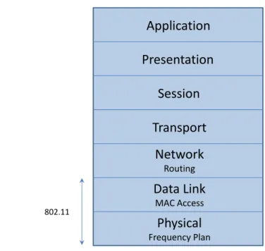
(WLAN) are the most important technologies for wireless broadband access. Network layout and its configuration influence overall performance of a spe-cific WLAN. For designing an efficient WLAN is necessary to carefully plan coverage and to optimize the network design parameter, such as AP locations, channel assignment, AP power allocation, MAC protocol, routing, etc... In the past, planning of the network was conceived as a static task. Now, in an heterogeneous radio environment, with mobile nodes, and conditions that are constantly changing, is necessary to apply dynamic network reconfigurability (for example [1]) featuring software defined radio [2, 3, 4, 5], arriving to nodes equipped with hardware card performing programmable MAC protocols [6]. In this thesis several algorithms for improving network’s performance in mesh and ah-hoc networks at different layers of the OSI model (showed in fig.1) are proposed: starting from an algorithm for identifying the channel quality that could be used as metric for applying routing algorithms (layer 3), passing for two algorithms for improving MAC access (layer 2), arriving to the physical layer with frequency planning (layer 1).

At the Routing Layer, link quality is considered a performance metric in dif-ferent protocols: in [7] Link Quality Source Routing (LQSR) is presented, that select a routing path according to link quality metrics; in this paper three different performance metrics compared with minimum hop-count

(15)

Application

Presentation

Session

Transport

Network

Routing

Data Link

MAC Access

Physical

Frequency Plan 802.11

Figure 1: The 7 Layers of the OSI Model.

ric are presented, but in a mobile environment minimum hop-count metric has achieved the best performance. In [8] a multi-radio LQSR taking into account both link quality and minimum hop-count metrics is proposed. An-other proposal is Multi-Path routing [10], that tries to perform load balancing and high fault tolerance selecting multiple path between source and destina-tion. When a link is broken on a path can be chosen another path in the set of existing path. A drawback of this protocol is the complexity. In [9] a hier-archical routing is presented, that proposes to divide nodes in groups. Each cluster has one or more cluster heads. Some node can communicate with more clusters, acting as gateway, to maintain connectivity. In high density networks this algorithm gives good performance, but the complexity of main-taining hierarchy and cluster heads that could be bottleneck may degrade the performance of the routing protocol. Another class of routing protocol pro-posed is geographic routing, in which packets are forwarded using only the position of neighbor nodes and destination node obtained through GPS or similar location techniques. Topology change has less impact in this protocol

(16)

with respect to the others, but packet delivery is not granted even if a path exists between source and destination. In order to guarantee delivery, planar-graph-based geographic routing algorithm has also been proposed [11], but they require much higher communication overhead.

It has been shown that in literature an important metric in routing algorithm is the link quality. In this thesis we present an identification algorithm based on an Hybrid Linear Varying Parameter model of a network that could be used for evaluate instantaneous bandwidth, i.e. link quality, that could be used as metric in a routing algorithm.

WLAN are based on IEEE802.11 standard family, that is divided into two main layers: Medium Access Control layer (MAC) and Physical Layer (PHY). A MAC protocol decides which nodes can transmit data at each time instant in order to avoid that two active links interfere with each other. The origi-nal 802.11 CSMA/CA Medium Access Control (MAC) has shown significant shortcomings when facing the breakthrough rate improvements made avail-able by the latest PHY enhancements (802.11n, 802.11ac), as well as when applied to scenarios and contexts such as ad hoc and mesh networks, ve-hicular environments, directional antennas, quality of service support, real time media streaming support, multi-channel operation, dynamic spectrum access, and many others. Designing high-performance MAC algorithms to achieve maximum possible throughput in WLAN is of primary importance. Since in many networks, especially when formed by a big number of nodes it is not possible to have a centralized control and resources at nodes could be limited, MAC protocol should be distributed and have low complexity and overhead. In literature there are a great number of proposed solutions: Max-imum Weight Scheduling (MWS) algorithm is based on length of the queue in each nodes [12], it is throughput optimal but requires to solve NP-hard optimization problem in a centralized manner at each time slot. An alter-native to this protocol with lower complexity is Longest-Queue-First (LQF) Scheduling. This algorithm schedule first nodes with longer queues disabling interfering nodes. It has demonstrated [13] that when topology network satisfy a local-pooling condition this algorithm obtains good performance in terms of throughput and delay, but in general topology it could not achieve optimal performance [14, 15] and when the size of the network grows also the

(17)

signaling and the time overhead can increase [16]. The most used protocols in wireless networks are Carrier Sense Multiple Access CSMA/CA algorithms. Applying these protocols in a distributed manner is very simple and they give good performance, but in presence ofhidden terminal nodes, nodes that are in visibility with receiver node but not in reciprocal visibility, the performance could severely degrade. In [17] an analytical model is derived to calculate the throughput of a CSMA-type algorithm in multi-hop wireless networks describing the evolution of schedules through a Markov chain. Based on this result, a distributed algorithm was developed in [18] to adaptively choose the CSMA parameters to meet the traffic demand without explicitly know-ing the arrival rates. On the basis of results in [17, 18], [19] proposes a discrete-time distributed queue-length based CSMA/CA protocol that com-bine CSMA with distributed GMS leading to collision free data transmission schedules. Another direction of designing CSMA algorithms for better delay performance is to use actual or virtual multi-channels, which is motivated by resolving the temporal link starvation of CSMA via de-correlating the temporal accessibility to the wireless medium. In [20] a CSMA algorithm with multiple frequency agility is presented, such that more than one fre-quency channel is available and a link can transmit on at most one of the channels. [21] proposes an algorithm called VMC-CSMA in which multiple virtual channels (defined by dividing the time line) are used to emulate a multi-channel system and address the starvation problem. The algorithm randomly selects a virtual channel, and the schedule corresponding to this chosen channel is used at each time slot. In [35] a fully-distributed CSMA based MAC protocol is presented. Employing virtual multi-channels it ob-tains good performance both in terms of throughput and delay in general wireless networks. Another class of MAC algorithms is Time Division Mul-tiple Access (TDMA) in which transmission of each node is scheduled in a different time slot. This class of protocols avoids collisions, but may lead to channel wastes. In this thesis we propose two algorithms for MAC access based on a combination between TDMA and CSMA algorithms. We divide the nodes in subnets, scheduling transmissions of subnets in different time slots, and performing CSMA behind a subnet.

(18)

is the frequency assignment. The problem was brought into focus with the introduction of the second generation (2G) cellular networks; in particu-lar, Global System for Mobile Communications (GSM) networks, that use a combination of Frequency Division Multiple Access (FDMA), TDMA, and random access. Frequency assignment problem could be approached in dif-ferent ways [22, 23, 25, 27, 28, 32, 34]. The basic approach is finding a frequency assignment which is feasible to assignment constraints and inter-ference constraints. Other approaches are the minimum interinter-ference problem and the minimum span frequency assignment problem. In the first problem, co-channel and adjacent channel interference are minimized. The second problem minimizes the difference between the highest and the lowest fre-quency used in solution. Frefre-quency assignment is typically viewed as a graph coloring problem [26, 27]. [29, 33] propose a cross-layer design and optimiza-tion considering the informaoptimiza-tion flows across the network layers to enable so-lutions that are globally optimal to the entire system and thus facilitating the optimal layer design. [24, 30] present another approach, considering layering as optimization decomposition, in which the overall optimization problem is decomposed in in subproblems corresponding to each layer. The inter-faces among layers are quantified as functions of the optimization variables coordinating the subproblems. In this thesis we present a fully-distributed frequency planning based on a machine learning mechanism, in which each node chooses autonomously and automatically the transmission channel. The remainder of the thesis is organized in three parts, respectively, address-ing the above described issues related to WLAN networks:

• In the first chapter an HLPV algorithm for identifying link quality [66, 68] is presented. We consider a hybrid model for the flow of traffic in communication networks, and identifying the region in which the link is working we could evaluate its instantaneous bandwidth.

• In the second chapter two MAC algorithms are presented, in the first [67] we propose a simple approach based on preallocating temporal slots in which different sets of nodes are allowed to contend for the channel access. Since the approach does not completely prevent contentions for accessing the wireless channel, we also propose a game-theoretical

(19)

analysis of contention strategies for multi-hop networks. In the second algorithm [69] we propose to convenient partition the network, applying an optimization algorithm for resource allocation.

• In the third chapter we propose a novel protocol [108] based on a dis-tributed machine learning mechanism in which the nodes choose, auto-matically and autonomously in each time slot, the optimal channel for transmitting through a weighted combination of protocols.

(20)

Chapter 1

HLPV Identification in wireless

ad-hoc networks

1.1

Introduction

Wireless ad-hoc networks consist of a number of untethered nodes able to communicate with each other by means of intermediate nodes, collaboratively forwarding ongoing traffic. Because of the nature of the wireless medium, data communications in ad-hoc networks are intrinsically broadcast, so that links exist between any pairs of nodes that are within the transmission range of each other. These features make ad-hoc networks easy to be deployed and suitable for a large number of applications, spanning from low-range sensor networks targeted to distributed monitoring, to high-range mesh networks targeted to build infrastructure-less transport networks.

In a WLAN, ensure that each node is aware of the performance of a link, allows the routing algorithm to make optimal decisions in case it is possible to reach a destination cross multiple path. Otherwise nodes should base their knowledge exclusively on static information. In this chapter we present an HLPV identification algorithm that could be used for evaluating link quality in wireless ad-hoc networks. We start our analysis from a model presented in [51] in which the flow of traffic in communication networks is modeled using a Hybrid System, which combines continuous-time dynamics with event-based

(21)

logic. Linear Parameter Varying, Hybrid Switching and Piece-Wise Affine models arise from different applications and have been studied in connection to various control schemes. Linear models allow for efficient design and soft-ware tools but often fail to provide a faithful description of the real systems. The use of LPV models as an approximation of nonlinear models became popular in the nineties [36]. In literature, a large amount of work on LPV control design and methods to obtain a set of stabilizing controllers pro-liferated since then. Actually, many industrial and advanced applications benefit the use of such techniques. Identification of LPV models has been approached since then in various way, by using State Space (SS) [37], [38], [39], Input/Output (I/O) [40], [41], representation The terminology Linear Parameter time-Varying (LPV) systems has been introduced in [36]. A dis-crete LPV system is represented in SS as

xk+1 = A(p(k))xk+B(p(k))uk

yk = C(p(k))xk+D(p(k))uk

The exogenous parameter p(k) is assumed a priori unknown. However, it can be measured or estimated upon operation of the system. Rather than modeling the dynamical evolution of a particular variable, one can treat it as an exogenous independent parameter, [36], [42], and the survey [43], as well as reference therein. Since the beginning of the nineties, the literature on LPV Control and LPV Identification has started growing almost in parallel. The first attempt to solve the problem of LPV identification dates back to the paper of [38], where Linear Fractional Transformation (LFT) LPV system identification problem is solved having single time-varying block and state space measurements. The problem was shown to be equivalent to a linear regression, and certain conservative conditions for persistence of excitation were given.

Since the end of the last century, the literature on LPV have tremendously been spread and it is almost impossible to exhaustively list all the contribu-tions here, but the main methodologies can be clustered according to various paradigm and criteria, in [44] an overview of all the approach of LPV identi-fication and more recent solved problems has been presented. On the other

(22)

hand, the importance of switching and hybrid dynamical systems [45] has been recognized, relying also upon the fact that robust stabilizing control can be designed, and new identification technique have been extensively con-sidered in the literature, [46], [47]. Hybrid systems are dynamical systems consisting of components with continuous and discrete behavior and thus they have required a new hybrid systems and control theory that has been developed in the past years and is still an active research topic. A survey of the principal identification methods for hybrid systems can be found in [46], [48] and [49]. An interesting paper that deals with an identification problem close to the one discussed here is [50]. In the rest of the chapter we present an application of HLPV in ad-hoc networks.

1.2

Model

1.2.1

System Model

The network structure can be represented through an edge labeled graph

G= (V, E). Specifically, the nodesetV includes all the nodesiof the network and the edgeset E includes all the pairs of adjacent nodes (i, j) that are in radio visibility of each other. We call each edge (i, j) ∈ E as link `, that is labeled with its maximum transmission rate Bmax reached only when we

are in the best condition. B` _≤_B

max is the effective transmission rate, that

in real environment is not constant over time, and depends on nearby radio conditions, and among the other factors, is function of the distance between nodes i and j and of the possible presence of obstacles.

1.2.2

Traffic Model

To model the channel traffic load, we take into account and extend the model originally proposed by [51]. For a given topology, we consider some of the nodes as sources and some are considered the final receivers. Actually we consider that the routing of the flows has been set, so for each flow the path is pre-assigned. We consider a communication network, with nl links, that

(23)

we assume unidirectional, crossed by n flows. Each link has a finite buffer, so when the queue reaches its maximum value the incoming packets will be dropped. In each link we define four vectors: q` that represents link’s queue value, s` is the rate packets arriving at the nodej for the link` that connects nodesj andk,r` is the transmission rate through the link andd`is drop rate at link `. Component f of these vectors is the contribution of the flow f to the total value. We neglect drops that occur in transmission medium. In this model the input variable is s`, the state variable q`, and the output is the transmission rate at the link `, y = r`. We can model the queue dynamics as: ˙ q` =s`−h(s`)−k(s`, q`) y= r`_f0 Where d`₌_h₍_s`_{) and} _r` f =k(s`, q`).

According to [51], queue dynamics can be described with a system in which, we use three different models depending of the value ofPn

i=1q ` f iand Pn i=1s l f i.

As showed in fig. 1.1, these are the parameters that allow us to transit from a state to another. In each case the expression of h and k will be different and the dependence ons` andq`changes depending on the different dynamic state of the queue:

• Queue Empty - Pn

f=1q`f = 0 : in this case there are no drops and all

incoming packets are transmitted. In this case we have : ˙ q` =s`−k(s`) Where kf i(s`) =    s`_f, Pn f=1s ` f ≤B ` B` s`f Pn f=1s`f , Pn f=1s`f > B` • Queue neither empty nor full - 0<Pn

f=1q ` f < qmax` or Pn f=1q ` f = q` max and Pn f=1s `

(24)

packets are transmitted at the head of the queue (B` bytes per unit of times). In this case we can rewrite the dynamics as:

˙ q` =s`−k(q`) Where kf(q`) =B` q` f Pn f=1q ` f • Queue full - Pn f=1q ` f ≥ q`max and Pn f=1s `

f > B` : in this case the

packets are transmitted at the head of the queue as in the previous case, but all the packets that exceed the maximum value of the queue will be dropped. In this case:

˙ q` =s`−h(s`)−k(q`) Where h(s`) =s`−B` s ` f i Pn f=1s ` f kf(q`) =B` q` f Pn f=1q ` f

Interest in the identification and validation of this model derives by the im-portance of on-line estimate the traffic load and the effective value of the bandwidth in the network, to implement a distributed optimization enhanc-ing performance in multi-hop transmissions.

Aim of this chapter is to show how to recast and identify such hybrid model as Hybrid LPV (HLPV). Interpret the behavior of a complex system as the effect of a linear model and a scheduling variable describing nonlinearity.

1.3

HLPV identification of the traffic model

According to [59] and [60], the literature can be divided into two main groups: identification methods based on state space (SS) vs. Input/Output (I/O) models, referring to the structure of the identified model. We can divide also

(25)

hybrid models in state space (SS) and Input/Output (I/O) representation. We focus our attention on the second one.

Equivalence among SS and I/O and proper discretization have been exten-sively discussed in literature, [53], then we notice that it is also easy to extend the above regressor to include the past terms of pk, such as pk−1, pk−2, .., as

required. In Piece-Wise-Affine (PWA) systems, [54], σk is given by

σk =i iff " xk uk # ∈Ωi, i= 1, . . . , s (1.1)

Following the discussion in [53, 55, 56, 57] a meaningful I/O representation of an HLPV model is the following one: Definition HLPVIO

y(k) =− na X i=1 (aiρk)y(k−i) + nb X j=0 (bjρk)u(k−j −d) +g(ρk) (1.2)

where ρk = [pk, σk], and denotes the evaluation of a function f over the

trajectory of ρk, i.e. f ρk = f(pk, pk−1, pk−2, . . . pk−ˆn, σk−ˆn, . . . , σk) (see

[53]) with ˆn = max4 {na, nb} and g a function taking into account the affine

terms. In some cases, the selected I/O description can be simplified consid-ering special forms of dynamic dependence on p, [58] allowing SS realizations without introducing dynamic dependence onp. The selected I/O description is appealing to describe the behavior of many practical applications and to derive a corresponding SS representation. The importance of subsequently determining a suitable SS representation is due to the fact that many effi-cient control techniques are formulated using state space information. An LPV model is characterized by the measurability of the scheduling variables. Then, under the assumption of measurability of ρk, it would be possible to

proceed in the solution of the identification problem. Indeed, for several applications it is possible to include additional information concerning the scheduling variables. First we want to show how to simply recast the wireless ad Hoc traffic hybrid model as HLPV. We consider a single link ` and we assume that the numbern of data flows is known and fixed to its maximum, which is equal to the number Ns of sources. Note that this is a restrictive

(26)

assumption because in general n can be also time-varying, n ∈ [0, Ns]. We

drop the superscript ` for sake of clarity. Such a hybrid model can be recast as a hybrid LPV model, by defining p1 := Pn

i=1qf i and p2 :=

Pn

i=1sf i and

assuming that the parameter p= [p1 p2]0 is the measurable varying param-eter. This parameter takes into account an aggregated value of the queue and the total incoming flow rate to the link. For each link the input is the

n−dimensional vectoru=sin which every components is random with uni-tary variance, the state is the n-dimensionalx=q and the measured output is given by the n-dimensional vector z = [zi] where

zi =yi+v, i= 1, . . . , n

and v is a measuring noise equally distributed on each flowfi. Moreover, we

assume that the theoretical value of the band B` =Bmax is known and the

maximum value of the queue qmax, but the effective value assumed by the

band is unknown and we rename it as bw ∈ [Bmin Bmax]. We assume that

the condition of an empty queue corresponds to p1 < , with sufficiently small.

Numerical simulations have been carried out to gather data with Bmin =

6M bit, Bmax = 54M bit, = 0.0001, and qmax = 0.03M bit. We consider

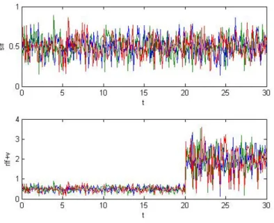
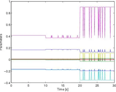
three flows crossing a link. The system is simulated in continuous time, but parameters are kept constant during sampling time and data have been collected at each sampling time interval. The corresponding simulated data are shown in Figure 1.2, for each flow (i= 1,2,3). The measured output is obtained by adding a uniform random noise v with unitary variance to the outputy. The simulation duration is 30s and the sampling time isT = 0.1s. The above hybrid model assumes the following HLP VSS form:

˙

x = A(ρ)x+B(ρ)u y = C(ρ)x+D(ρ)u

z = y+v

(1.3)

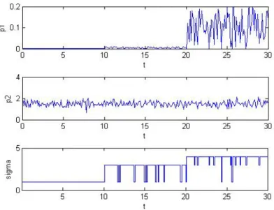
where ρ= [p0 σ]0 is the parameter vector and the switching parameter σ is defined as follow:

(27)

σ =σk =j, j ={1,2,3,4} ⇐⇒ p∈Ωj Ω =                    Ω1 if(p1≤ AND p2≤bw) Ω2 if(p1≤ AND p2> bw) Ω3 if( < p1< qmax) OR (p1 = qmax AND p2≤bw) Ω4 if(p1> qmax) OR (p1 = qmax AND p2> bw) (1.4)

In 1.4 the sets introduced are related to the dynamical model introduced in section 1,Ω1 is the region corresponding to the condition queue empty, Ω3

queue neither empty nor full, Ω4 queue full. Ω2 is a degenerate region, a

point between Ω1 and Ω3. Note that the above regions are depending on the

unknown parameterbw. Actually we use a first approximation of this regions

where the known maximum value of the band Bmax, instead of the effective

value bw is used.

Notice that, because the particular structure of the model, all the ma-trices become diagonal mama-trices with the same entries for i = 1, . . . , n:

A = diag(ai) = diag(a),B = diag(bi) = diag(b), C = diag(ci) = diag(c)

and D =diag(di) =diag(d) with:

a(ρ) = ( 0 if j = 1,2 −bw p1 if j = 3,4 b(ρ) =            0 if j = 1 1−bw p2 if j = 2 1 if j = 3 bw p2 if j = 4 c(ρ) = ( 0 if j = 1,2 bw p1 if j = 3,4

(28)

d(ρ) =      1 if j = 1 bw p2 if j = 2 0 if j = 3,4

Because the above state space model is diagonal and the entry terms are all the same, a first order scalar state-space model for each single flow, Σ =

{a(ρ), b(ρ), c(ρ), d(ρ)} can be taken into account by itself.

For the present example, the parameters are kept constant during the sam-pling time interval, so that the switching can occur only at the samsam-pling time instant and then, both the I/O representation and the discrete-time model can be easily derived. The corresponding continuous time input-output model is obtained simply by deriving the input-output expression and sub-stituting the derivative term ˙x:

γ(ρ) ˙yi(t) =α(ρ,ρ˙)yi(t) + (β(ρ))ui(t) where γ(ρ) = ( 0 if j = 1,2 1 if j = 3,4 α(ρ,ρ˙) = ( c(ρ) if j = 1,2 a(ρ)− p_p˙1₁ if j = 3,4 and β(ρ) = ( d(ρ) if j = 1,2 c(ρ)b(ρ) if j = 3,4

The discretization of the former model, via a backward Euler approximation with a ZOH, gives raise to a simple HLPVIO:

A(δ, ρk, ρk−1)yi(k) =B(δ, ρk)ui(k) (1.5)

where A(δ, ρk, ρk−1) = a0(ρk, ρk−1) +a1(ρk)δ and B(δ, ρk) = b0(ρk) and the

(29)

follows: a0(ρk, ρk−1) = ( 1 if j = 1,2 (2−T a(ρk))p1k−p1k−1 if j = 3,4 a1(ρk) = ( 0 if j = 1,2 p1k if j = 3,4 b0(ρk) = ( d(ρk) if j = 1,2 T c(ρk)b(ρk)p1k if j = 3,4

Clearly, the functional dependence on ρk, ρk−1 is unknown and is one of the

object of the identification. Moreover, model (1.5) can be easily recast with the structure given in (1.2) as

y(k) = (α1ρk)y(k−1) + (α0ρk)u(k),

with (α1ρk) = α1(p1k, p1k−1, σk) and (β0ρk) = β0(p1k, p2k, p1k−1, σk).

Depending on the available a-priori information on the model, some possible different identification solutions can be adopted, as described in [44] Here we report the application of the following solution. Off line identification. Assume that the regions are known. Design the identification experiment choosing the input at the sources, measuring p2 at each link and selecting the variation of p1 satisfying the persistence excitations conditions as in [52]. Divide the data according to each region j and use the standard I/O LPV identification method, recasting model (1.5) in a psuedo-regressor form and identify each LPV model corresponding to a value of j.

1.4

Numerical Results

We now explain our results, mediated over seven simulations. Actually our goal is identify the model to validate it, in future works we consider identi-fication of the effective band bw, considering the regions unknown. In each

(30)

have performed Least Mean Square algorithm. We consider

B(δ, ρ) := b0(ρ) +b1(ρ)δ+. . .+bnb(ρ)δ

nb

A(δ, ρ) := I+a1(ρ)δ+. . .+ana(ρ)δ

na _(1.6)

with na = 2 and nb = 1. For ai and bi we choose polynomial functional

dependence for the parameters:

ai(ρ) = a1i +ai2ρ+. . .+aNi ρN−1

bj(ρ) = b1j +bj2ρ+. . .+bNj ρN−1.

(1.7)

with N = 3. So in each region we have identified the coefficients in the matrices: Θ :=      a1 1 a21 a31 a1 2 a22 a32 b1 0 b20 b30 b1 1 b21 b31     

In Figure 1.4, Figure 1.5, and Figure 1.6 we see the simulation results of LMS algorithm in regions 1,3 and 4 respectively.

We underline that we do not have identification in region 2, this is because region 2 is a degenerate region i.e. a point, and using random input, guar-anteeing persistence of excitation, we have not crossed this region. The convergence values of the coefficients in the regions (in the figures we see only the first part of the simulation and not the convergence) are:

Θ1 :=      −0.1642 0 0 −0.1846 0 0 0.3903 0 0 0.1643 0 0      Θ3 :=      −0.1684 0 0 −0.1902 0 0 0.3530 0 0 0.1716 0 0     

(31)

Θ4 :=      −0.2135 −0.0245 0 −0.3603 −0.0374 0 0.7993 0.1030 0 0.1319 0 0     

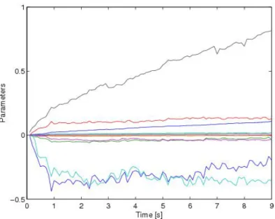
In Figure 1.7 we see the global identification, i.e. we see parameters crossing the different regions during the simulation’s time. In this figure we see the convergence value of previous figures.

1.5

Future Works

HLPV models inherit properties of LPV and PWA affine systems with the addition of some knowledge on the scheduling variables.

A possible off line identification algorithm has been implemented. Other more efficient solutions need to be investigated. We list now possible future algorithms that need to be implemented.

1) On line identification.

a) Assume that the regions are known. Design the identification ex-periment choosing the input at the sources, measuring p2 at each link, and selecting the variation ofp1 satisfying the constraintsC.1 andC.2 and the persistence excitations conditions as in [52], and, at the same time, guaranteeing that the parameterσ is kept con-stant in a sufficiently long time to guarantee convergence of the al-gorithm. Then, use the standard I/O LPV identification method, recasting model (1.5) in a psuedo-regressor form and identify each LPV model.

b) Assume that the regions are not known, but the number s = 4 is known. Design an identification experiment as in 2a). A posteriori, separate each LPV model, from the identified one. 2) Two step identification. Assume that the approximating regions need

(32)

on p, to find approximated regions and validate them. Second, run one of the previous identification scheme 1) or 2). This solution is still under investigation.

3) Global experiment. In case we would like to perform an on line identifi-cation and the assumption that σ is kept constant in a sufficiently long time cannot be guaranteed, or if the model is more general than the one obtained in the present example, then a global experiment for the model given as in (1.2) need to be performed. A suitable identification algorithm determining in one-shot both the functional dependence on

p and on σ need to be performed. This general solution is still under investigation.

(33)

Figure 1.1: Hybrid Model for the queue at a link. Source: [51]

Figure 1.2: Input/output data over an interval of 30s and sampling time T=0.1s for each flow i= 1,2,3.

(34)

Figure 1.3: Parameters p1, p2 and σ over an interval of 30s and sampling time T = 0.1s.

(35)

Figure 1.5: Parameters’ identification in region 3.

(36)

(37)

Chapter 2

Medium Access: Contention vs.

Scheduling

2.1

Introduction

In wireless networks is of primary importance deciding when a node can send a packet, and when it have to listen for receiving a packet. Making the right decision could be difficult and could cause medium wastes and degradation of network’s performance in terms of throughput. We consider solutions which are centralized or distributed. Centralized solutions as polling and TDMA (Time Division Multiple Access) with a centralized computation are simple and they guarantee total absence of collisions, but are applicable only in small and trivial networks. In greater networks we have to consider dis-tributed algorithms that could be equipped with schedule-based protocols or

contention-based protocols. In schedule-based protocols the node to be trans-mitted is regulated in each time; scheduling could be fixed or on demand. This approach needs a synchronization mechanism. Most ad-hoc networks rely on contention-based medium access protocols, since the use of carrier sense and random backoff mechanisms is a simple and well-established solu-tion for distributedly managing multiple-access over a shared channel band-width. However, it is well known thatCSMA/CA (Carrier Sense Multiple Access/Collision Avoidance)protocols exhibit very poor performance in case

(38)

of multi-hop transmissions. This is due to the inter-link interference caused by imperfect carrier sensing, i.e. the impossibility that a transmitter detects a signal interfering to the intended receiver and originating from a node out of its carrier-sense range. The collisions due to this phenomenon, called hidden-node collisions, can severely degrade the network throughput as the transmission rate of each node increases. Theoretical bounds on the attain-able limits of throughput in presence of imperfect carrier sensing have been studied. In the seminal paper [61] bounds were determined for a network with arbitrarily or randomly deployed nodes under the assumption that an ideal scheduling scheme for arbitrating node transmissions can be implemented. In [62] some analysis extensions have been considered for quantifying the impact of mobility and node cooperation on such bounds. The hidden ter-minal problem of CSMA/CA protocol is addressed in many papers, i.e. [63]. Moreover, in [64] a time-division scheduling for ad-hoc networks is presented, with an analysis of the TDMA policy. Apart from the bound identification, a crucial problem for actual network deployments is the implementation of an efficient node coordination scheme. The scheme must be able to minimize the signaling overhead required for coordinating multiple node transmissions, while guaranteeing a significant performance improvement over CSMA/CA protocols. For improving CSMA performance has been presented several pa-per based on the idea of adapting contention aggressiveness basing on the basis of queue’s length [65],[70],[71],[72]. Motivated by the study in [73] in which has proved that this approach can suffer high performance degradation because of channel asymmetries, packet collisions at flow receivers and dy-namic traffic pattern, [74] proposes a system for proportional fairness keeping in count optimization and robustness. They relax the assumption of chan-nel symmetry and introduce a robustness function for reducing performance degradation due to collisions decreasing channel access for avoiding interfer-ence when the number of contending flows increase. A strong point of CSMA algorithms is the flexibility in adapting when network’s conditions change in topology or in traffic load. In order to become competitive, scheduled pro-tocols should have a continuous adaptation method. In [76] and [77] it has been proposed to alternate a contention phase and a scheduled phase. In the first phase nodes exchange topology information that are used for

(39)

comput-ing the schedulcomput-ing in the next phase. The problem in this approach is that change in topology or traffic load could not be aligned with the phases of the algorithm. In [79] a topological allocation through a distributed algorithm that can operate within scheduled and contention-based MAC protocols is proposed. This algorithm evaluates node’s topological persistence that is the fraction of time that it is permitted to transmit, and after identifying ideal persistences for a given topology and traffic load, topological persistences is given as input to MAC protocols. This approach has several limitations: the algorithm assumes a priori knowledge of traffic demands and local topology; it does not accommodate changes in topology or traffic demands; the algo-rithm requires synchronization. This algoalgo-rithm is improved in [78] in which node’s persistence is also computed but a scheduled MAC protocol able to adapt to change in topology and traffic load is presented. Our approach is to find a distributed resource allocation algorithm combining TDMA for group-ing contendgroup-ing nodes in non-interfergroup-ing sets and CSMA/CA for managgroup-ing the channel access behind a set. This pre-allocation mechanism of channel holding times can significantly reduce the channel wastes due to hidden node collisions and has been recently considered also in some standardization task groups working on mesh networks and literature, for optimizing both the net-work capacity and the energy consumption [80] in Zigbee netnet-works, or coping with bidirectional traffic flows over chain topologies exploiting network cod-ing [81]. In the rest of the chapter we focus on the problem of determincod-ing the optimal resources allocation, that is how many resources guarantee to each node in order to obtain the best performance in terms of throughput. The rest of the chapter is organized as follows:

• In section 3.4 we formulate the problem;

• In section 2.3 we present a solution that consists in scheduling poten-tially interfering transmissions in different time slots, while allowing in-range nodes to transmit in the same time slot but subject to a CSMA/CA mechanism that avoids collision. The problem is formu-lated in terms of a map coloring problem. Since color allocations may leave some level of contention, by assigning the same color to nodes in radio visibility, a game theoretical study of intra-slot contention is

(40)

introduced.

• Motivated by results obtained in section 2.3 showing that combining contention and scheduling gives an improvement on both approaches CSMA and TDMA, we asked ourselves what is the optimal degree be-tween contention and scheduling. We present an algorithm which finds a conveniently partition of the network, scheduling the transmissions of different subsets in different time-slots. We apply an optimization algorithm for deciding how many time-slots are guaranteed to each sub-net. The number of subsets giving the best performance in a particular network is the optimal degree between contention and scheduling for that network.

2.2

Problem Formulation

We consider a single channel radio network made of a set V of nodes dis-tributed uniformly over a given area. Each node i ∈ V can communicate only with a subset of adjacent nodes Vi. We say thatiis (radio) visible only

to the nodes in Vi. Differently, i is hidden to the remaining nodes in V \Vi.

We assume that radio visibility is symmetric and that the communication between pair (i, j) of adjacent nodes presents a maximum transmission rate

rij, function of the distance between nodes i and j and of the possible

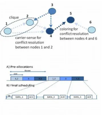
pres-ence of obstacles. The channel time is divided into elementary allocation units called slots. Each slot is able to accommodate a random backoff de-lay and the transmission time of the maximum allowed packet size at the minimum rate (followed by an explicit acknowledgment). Only the subset of nodes to which a generic channel slot is pre-allocated are enabled to perform the CSMA/CA function for transmitting on that slot. The slot allocations are maintained on a per-frame basis: being x the total number of alloca-tion slots, a sequence of xconsecutive slots is a channel frame in which, slot by slot, the same sorted list of nodes are enabled to transmit. Figure 2.1 shows an example of medium access in a network with 5 nodes, in which a channel frame of 3 slots is considered. In the first slot, where only station 1 and 2 can access the medium, station 1 wins the contention (i.e. extracts

(41)

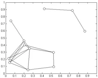
Figure 2.1: An example of medium access in a network with 5 nodes and a frame composed of 3 slots.

the lowest backoff delay). The second slot is used by station 3 only, while the third slot is reserved to the contention between stations 4 and 5. The reason for pre-allocating channel slots to a sub-set of stations (thus grouping in independent sets the stations allowed to transmit simultaneously) is the mitigation of the hidden node problem. For example, if stations 1 and 3 are hidden to each other (as shown in the figure) and wish to transmit to station 2 (which is able to hear both the stations), the previous allocation avoids any collision possibility. Conversely, transmissions originated by stations 1 and 2, which are in reciprocal visibility, are separated by the CSMA/CA protocol. We formally define the problem of slot allocations in what follows.

2.2.1

Network Structure and Traffic Model

We represent the network structure through an edge labeled graph G = (V, E). Specifically, the nodeset V includes all the nodes i of the network

(42)

and the edgeset E includes all the pairs of adjacent nodes (i, j) that are in radio visibility to each other. Each edge (i, j) ∈ E is labeled with its maximum transmission rate rij.

Since the system time is slotted, we also model the traffic source at each node in terms of per-slot packet probability. Specifically, we assume that each node i has a fixed probability λi to generate a packet in each slot.

In order to avoid interactions with the routing protocol, we consider only one-hop packet deliveries. Packets are destined to a randomly selected node among the neighbor ones. For isolated nodes, i.e. nodes without neighbors, the traffic is assumed to be broadcast. In addition, we assume that the packet size is of a fixed valueDfor all the nodes, whose transmission time is always compatible with the slot size.

2.2.2

Resource Allocation

We assume that the reader is familiar with CSMA/CA protocols, which regu-late the final channel access within an allocated channel slot. Although most CSMA/CA protocols use a slotted backoff scale for efficiency reasons and for implementation limits (since the carrier sense cannot be instantaneous), we assume that backoff values are uniformly extracted in a continuous range [0, b], thus implying that collisions cannot be originated by the extraction of two identical backoff values. In order to implement a slot allocation mech-anism, two basic functionalities have to be provided in the network: i) a mechanism for inferring the network topology; ii) a mechanism for keeping a common time reference among the nodes. For both the aspects, we consider that an independent signaling channel is available (managed by a random access scheme) and nodes in radio visibility can exchange control informa-tion (e.g. the list of neighbor nodes). We also assume that nodes do not have data storage constraints, while processing capabilities may depend on the specific network scenario.

(43)

2.3

Utility-Based Resource Allocations in

Multi-Hop Networks

In this section, the problem is formulated in terms of a map coloring prob-lem, which has a vast and well established literature [83, 84]. Therefore, we simply adapt some existing coloring algorithms to ad-hoc networks, by trying to identify the most effective trade-offs between complexity, signaling over-heads and performance gain. Since color allocations may leave some level of contention, by assigning the same color to nodes in radio visibility, a game theoretical study of intra-slot contention is also introduced. In the above context, the two main problems of our interest are the following ones.

Problem 1. Determine a distributed protocol that sets the number x of slots in a frame and the slots allocations, in order to maximize the per-node throughput in saturation conditions, i.e. in presence of greedy sources whose packet generation rate is λi = 1.

Problem 2. Determine a distributed protocol that allows the allocations of slots of a frame in order to minimize the average delivery delay for generic source rates λi.

2.3.1

Solution Approach

In this section, we discuss the possibility of reducing Problems 3 and 4 to a set of Minimum Graph Coloring (MGC) problems.

2.3.2

Graph coloring

LetG(V, E) the network graph including the setV of nodes distributed over a given area and the setEof edges connecting radio visible nodes. Each node

i ∈ V is labeled with the number ai of slots to be allocated to it according

to the traffic it must support. Generally speaking a single slot is allocated to each node. However, in case of heterogeneous packet generation rates

(44)

paths and aggregating traffic packets generated by multiple sources), some nodes may require more slots to drain their traffic.

We define as incompatibility graph of type I the node labeled graphHE(V, FE)

whose edges in FE join the pair of nodes (j, k) ∈ V ×V whose frames may

collide if transmitted simultaneously. By definition HE =G2, that is,

FE ={(j, k) :∃i∈V s.t. (j, i),(i, k)∈E}.

We can see Problems 3 and 4 as a MGC problem that determines the min-imum cardinality of a coloring of the nodes of HE such that each node is

colored with as many different colors as its label. Then, each color corre-sponds to a specific slot allocated to the node on the frame.

Obviously, the network transport capacity is critically affected by the car-dinality x of a coloring of HE, since each node i receives ai transmission

chance only every x slots. For example, assuming a uniform transmission rate r among all the edges, the node transmission rate is upper bounded by

ai·r/x.

In defining the incompatibility graph of type I, we have not considered the carrier sense functionality that intrinsically makes orthogonal (i.e. non-interfering) the transmissions between visible nodes. Edges connecting visible nodes in the incompatibility graph of type I may result redundant and some, if not all of them, may be removed, possibly drastically reducing the number of colors necessary for the graph. In this context, we define as incompatibility graph of type II the node labeled graphH∅(V, F∅) whose edges in F join the pair of nodes (j, k) ∈ V ×V that are of the reciprocally hidden and whose frames may collide if transmitted simultaneously. By definitionH∅ =G2−G, that is,

F∅ ={(j, k) :∃i∈V s.t. (j, i),(i, k)∈E but (j, k)6∈E}.

Removing edges from the incompatibility graph can make the per-node trans-mission rateSi (also called node throughput) heterogeneous, even in the case

(45)

with visible nods receive a throughput bounded byai·r/x, while nodes

shar-ing the slot with neighbor nodes experience, in the worst case, a throughput reduction equal to the number of contending nodes.

The graph HE and H∅ define the two extreme cases in which either all or

none of the pair of reciprocally visible nodes are considered. Obviously, even intermediate situations may be defined. Let 2E _{be the power set of the}

edgeset E.

For eache∈2E, we can consider the coloring problems of the incompatibility graphsHe = (V, F∅∪e), and the per-node and aggregated throughput,Sieand

S_tote =P

i∈V S e

i. Then, the optimal coloring scheme is the coloring referring

to the incompatibility graphHewhich maximizes the value ofStote , fore∈2E.

2.3.3

Throughput assessment

Consider a He, for e ∈ 2E, graph. For each node i ∈ V, let us define its

associated after coloring clique as the maximal clique on the graph G that includes i and is formed by nodes of the same color of i. Let de_i be the size of such a clique and let ai = 1 ∀i.

Then, if we assume a uniform rate r for all the links in E, we can guarantee a per-node collision free throughput

ρe_i = r

xe_de i

(2.1)

where, xe _{is the number of colors used in} _H

e. The rationale behind (2.1) is

the following. For each nodei∈V, we have to share the slot associated to its allocated color withde

i−1 contending nodes. On average, nodeiwill win the

backoff contention only once every de

i frames. Collisions with adjacent nodes

are avoided by means of the carrier sense functionalities, while collisions with other nodes using the same colors are avoided by the coloring algorithm (which re-assign the same slot only when nodes are distant more than two hops).

(46)

by ∆e+ 1, where ∆e is the maximum node degree of the graph. In addition, coloring He with at maximum e + 1 colors can be easily attained with a

distributed protocol, such as Brooks-Vizing, [87]. The following condition then holds:

r

∆E₊₁ ≥ maxi∈V _(∆e₊₁₎r _de i

∀e∈2E

Since ∆e _{is an upper bound on the number of needed colors, the previous}

condition implies that the lower bound of the collision-free throughput guar-anteed to each node is higher for the incompatibility graph HE.

Let us now consider the aggregated collision-free throughput ρe_tot. After col-oring, the throughput sum perceived by all the nodes belonging to each clique is obviously r/xe, thus resulting in a total throughput equal to:

ρe_tot = r

xec e

where ce _{is the total number of cliques resulting from the coloring of the}

incompatibility graph He. Obviously, when He = HE such a number

corre-sponds to the number of nodesn(since 1-hop nodes are allocated on different channels). It follows that we can also express the average per-node through-put E[ρe_{] as}_ρe

tot/n= xe_Er_[_de_] (whereE[de] =n/cerepresents the average after

coloring clique size).

For each e∈2E_{, we note that the collision free throughput is only a}

guaran-teed lower bound on the actual throughput Se

tot that we can obtain coloring

the graphHe. In fact,Stote can be a higher throughput. Letxebe the number

of colors used for He. Consider a generic node i and let xi the number of

colors used for coloring its adjacent nodes on He. When xi < xe + 1, we

may obtain a transmission rate for i greater than the one guaranteed by the collision free throughput if we allow ito transmit during the slots associated to its color and to colors different form the ones of its adjacent nodes on

He. If i is the only node with such a privilege, we will obtain a throughput

(with no collision) higher than the collision free throughput. Differently, if we concede the above transmission privilege to all the nodes withxi < xe+ 1,

we cannot guarantee that extra slot allocations result in a free transmission. Nevertheless, we obtain an overall throughput higher than the collision free

(47)

throughput, as long as each node does not transmit to the slots associated to the adjacent nodes on He. If the competition for extra slots is extended

to all the slots of the frame (thus including the potential interfering nodes), the collision-free throughput cannot be guaranteed anymore. Therefore, we are currently investigating on the risks and benefits of enabling extra slot allocations, by means of a game-theoretical analysis.

2.3.4

Coloring Algorithms

Coloring algorithms have been widely explored In literature. Some examples of popular solutions are the Luby’s algorithm [85], the Johanson’s algorithm [86], and their variants [87].

We consider here the algorithm proposed in [75]. A preliminary exchange of control information is necessary for evaluating at each node i the global degree of the network ∆ or the local number of neighbors δi. Let xmax the

global or the local maximum number of available colors. According to the basic algorithm, each uncolored node has to perform the following steps:

1. First coloring Randomly pick a color from a list of available colors. 2. Conflict ResolutionIf none of your (1-hop or 2-hop) neighboring nodes

has chosen the same color, keep it as definitive color, otherwise remove it form the list and try again the next step.

3. List updateIf the color list is empty, add new colors. The list is updated

starting from min{c+1, xmax}color, wherec= max{neighboring node colors}.

This algorithm is called SC algorithm, for recalling its characteristic of first

Selecting a color and thenComparingthe selected color with potential inter-feres.

In order to optimize the number of used colors, we also considered a simple modification of the previous scheme. Instead of randomly picking a color from the available ones, each node first updates the list of available colors (as in the third step of the previous scheme) and then selects the color with

(48)

the lowest index. This scheme is called CFA algorithm, since it is based on

Choosing the First Available color. While the nodes belonging to different cliques cannot interfere because they are allowed to transmit only in different frame slots, nodes belonging to the same after-coloring clique can hear each other and have to use a CSMA protocol to share the same frame slot. In section 2.3.3 we have assumed that nodes sharing the same frame slot have the same probability to win the contention, i.e. in long terms they obtain the same number of transmission grants. However, this assumption can be restrictive. Indeed, nodes could be motivated in using heterogeneous access probabilities1 _{for delivering more traffic. For examples, nodes relaying traffic}

of many other nodes could need more channel resources than nodes trans-mitting only their own packets, for preventing buffer overflows and packet drops. Therefore, here we consider a game-theoretical analysis of intra-clique contention. While the impact of heterogeneous access probabilities have been considered for 1-hop wireless networks [88], according to our knowledge this problem has not been explicitly addressed for multi-hop networks.

2.3.5

Station Utility

We consider a set of N nodes belonging to the same clique and sharing the same frame slot. Let τi be the slot access probability (i.e. the node strategy)

and let λi be the per-slot packet generation probability of a generic station

i (with i= 1,2,· · ·N). Since we are not modeling traffic paths and routing schemes, we assume that λi takes into account both the node internal and

external (i.e. coming from other nodes) packet enqueuing rate and that each node selects (uniformly) all the neighbor nodes as relays. We also assume that during the network topology discovery phase, nodes exchange information about their traffic patterns, thus notifying the resulting λi values to the

neighbor nodes.

A key aspect to be investigated is the definition of the utility function driving

1_{Heterogeneous access probabilities can be supported by using a protocol such as the} IEEE 802.11 EDCA, which differentiates the channel access probabilities of different traffic classes, or by configuring non-standard access parameters by means of open-source drivers accessing the card configuration registers.

(49)

the configuration ofτi parameters. In single hop networks, such a utility has

been usually expressed in terms of transmission throughput percevied by each contending node. Beingpi = 1−

QN

j=1(1−τj)/(1−τi) the collision probability

suffered by stationibecause of other node channel accesses, the transmission throughputµi of stationican be expressed asτi(1−pi) packets/slot. Under a

utility function Ji =µi, the station best response corresponds to play τi = 1

and the channel resources can be completely wasted whenever at least two different stations play this strategy.

The transmission throughput has been already proved to be an inconsistent utility function for bi-directional traffic scenarios [88], where nodes are in-terested not only in transmitting the locally-generated traffic packets, but also in receiving the packets generated by the peer application. Therefore, it is even more inconsistent for multi-hop networks, where the transmission throughput of a given node directly affects the throughput of the neighbor nodes using such a node as a relay. In other words, nodes cannot be only interested in maximizing their transmission rate, since they need to leave re-sources to the neighbor nodes which will carry their traffic towards multi-hop destinations.

These considerations motivate the definition of a utility function describing the whole transport capacity of the clique. Since in our model each node of the clique exploits all the neighbor nodes as relay, we assume that the clique nodes are interested in avoiding buffer overflows or bottlenecks at each node of the system. In other words, being Qi the average queue length of node

i, we define Ji = −maxi=1,2,···NQi = J ∀i. Being K the buffer size of

each node (expressed in terms of maximum number of packets that can be accommodated in the buffer), we can express the average queue length of node i as: Qi = ( min{ λi µi−λi, K} µi > λi K µi ≤λi (2.2)

Since the queue length provides a negative utility (i.e. it represents a cost for the system in terms of pending packets to be delivered out of the clique), nodes have to minimize such a length in order to maximize their payoff.

(50)

2.3.6

Station Best Response

An important aspect of our utility function formulation is that such a function is common to all the stations, In fact, since each node has to relay on other nodes for ultimately delivering and receiving its own traffic, there is no point in implementing greedy behaviors that prevent neighbor nodes from accessing the allocated frame slot. Moreover, such a common utility, which represents the clique transport capacity, prevents other malicious behaviors such as the signaling of wrong traffic generation rates λi. Being the node induced to

collaborate by the need of maximizing a common utility, we also assume that in each notification message about neighbor nodes and traffic rates nodes can also announce their current strategy τi2.

Consider now a tagged node j of the clique. On the basis of the λi and

τi parameters signaled by all the clique nodes i = 1,2· · ·N i 6= j, and

on the basis of its traffic rate λj, the tagged node can implement a best

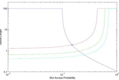
response strategy based on the evaluation of the per-node queue lengths as a function of the tagged node strategyτj. Figure 2.2 shows an example of such

evaluations in a scenario with four nodes in which all the traffic rates are constant and equal to 0.05 packets/slot and K = 100. The curves have been obtained assuming that the tagged node is node 1 and thatτ2= 0.15,τ3=0.2,

andτ4=0.25. WhileQ1 is a not increasing function ofτ1 (since increasing the

channel access rate node 1 has more chances to deliver its traffic), all the other queue functions are not decreasing (since neighbor nodes experience higher collision rates as the tagged node increases its access). For minimizing the maximum queue length of the system, node 1 has to play τ1 = τ2 = 0.15

that means that has to equalize its queue to the length of the worst neighbor queue. BeingQj(τj) not increasing withQj(0) =KandQi(τj) not decreasing

withQi(1) =K ∀i, that such an equalization it is always possible for at least

one strategy τj. Such a strategy is unique if the intersection point between

Qj and the highestQi curve is in the strictly monotoning range of the curves

(as shown in the figure), while it corresponds to a range of possible values when the intersection is on the flat region of the curves (i.e. for Qi =K). In

2_{Such a notification is in principle not necessary, since each node can independently} estimate the access probability of other nodes from channel observations.

(51)

Figure 2.2: Queue Length at each node, as a function of the strategy of a given contending node.

this last case, the tagged node could decide to play the highest τj value of

the range.

Generalizing the previous considerations to the case of heterogeneous λi

pa-rameters, we can implement a best response strategy as follows:

τ_jbr = ( λjτx λx−τx(λx−λj) Qx < K λj Q i6=j(1−τi) K+1 K Qx =K (2.3)

being x the index of the node experiencing the worst congestion (i.e. the longest queue). It can be proved that by repeating such a best response strategy for all the nodes at the reception of the announcement messages, in a finite number of steps the system converges towards a Nash Equilibrium (NE) point, in which all the clique queues are equalized. The equilibrium point is not unique and depends on the initial strategies of the nodes. The details of such analysis are in [82].

2.3.7

Numerical Results

(52)

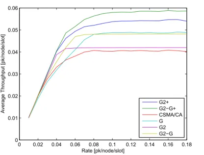
0 0.02 0.04 0.06 0.08 0.1 0.12 0.14 0.16 0.18 0 0.01 0.02 0.03 0.04 0.05 0.06 RateG[pk/node/slot] AverageGThroughputG[pk/node/slot] G2+ G2−G+ CSMA/CA G G2 G2−G

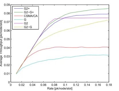
Figure 2.3: Average throughput under the SC coloring scheme, for different incompatibility graphs and comparison with standard CSMA/CA.

improving the CSMA/CA performance in multi-hop networks, we run sev-eral simulations, including both the network coloring phase and the data transmission phase. Obviously, the throughput performance perceived in a given network topology are critically affected by the final map of colors and by the node source rates. For the same network topology, such a final map depends on the random color selections and/or on the node initialization choices. Therefore, each run performance can be different and has to be av-eraged. Note also that in our simulations, we do not consider dynamic node activations and de-activations, thus running the coloring phase only at the beginning of the simulation and maintaining the color map for the rest of the simulation time.

We considered random network topologies of 30 nodes deployed over an area of 10·10m2, with a transmission range of 3m. We observed that the CFA scheme requires on average 15 different colors when the incompatibility graph isHE =G2, while it uses 8 colors only for the graphH∅ =G2−G. Conversely,

the SC coloring scheme resulted in an average number of colors equal to 24 for the G2 −G case, and 17 for the G2 −G case. The higher number of

(53)

adopted colors has two different effects: on one side it increases the frame length, thus resulting in a lower rate of node transmission chances; on the other side it reduces the contention level between 1-hop nodes in case of

G2−G.

After that each node has been colored, we simulated 5000 channel slots. At each slot, three different steps are considered: i) generation of traffic packets, ii) selection of transmitting nodes; iii) verification of transmission outcomes. At the first step, a new packet is generated in the transmission buffer of each node i with a fixed probability λi = Rate ∀i. The destination node is

uniformly extracted among the neighbors and no buffer size limit is consid-ered. At the second step, the simulator processes all the nodes whose color corresponds to the current slot and extracts uniformly a backoff value for resolving potential contentions. Since the traffic rate of each node is con-stant, the backoff range of each node is constant too, in order to implement a uniform slot access probability within the after-coloring cliques. All nodes winning the contention are labeled as transmitting. Finally, if the neighbors of the intended receiver are not transmitting, the transmission is considered successful and the packet is removed from the buffer. Otherwise, the packet remains in the buffer until a maximum number of retries (set to 3) has been reached.

Figures 2.3 and 2.4 compare the per-node average throughput measured in our simulations, under the SC and CFA scheme, for different incompatibility graphs (namely, G, G2 and G2 −G). In both the figures we also plot the CSMA/CA performance. The throughput has been averaged by considering te