Predicting the Resource Consumption of Network Intrusion Detection Systems

Predicting the Resource Consumption of

Network Intrusion Detection Systems

, Anja Feldmann2

, Vern Paxson3,4

, and Robin Sommer4,5 1

Siemens AG, Corporate Technology 2

Deutsche Telekom Labs / TU Berlin 3

UC Berkeley

4

International Computer Science Institute 5

Lawrence Berkeley National Laboratory

Abstract. When installing network intrusion detection systems (NIDSs), opera-tors are faced with a large number of parameters and analysis options for tuning trade-offs between detection accuracy versus resource requirements. In this work we set out to assist this process by understanding and predicting the CPU and memory consumption of such systems. We begin towards this goal by devising a general NIDS resource model to capture the ways in which CPU and memory us-age scale with changes in network traffic. We then use this model to predict the re-source demands of different configurations in specific environments. Finally, we present an approach to derive site-specific NIDS configurations that maximize the depth of analysis given predefined resource constraints. We validate our approach by applying it to the open-source Bro NIDS, testing the methodology using real network data, and developing a corresponding tool,nidsconf, that automati-cally derives a set of configurations suitable for a given environment based on a

sampleof the site’s traffic. While no automatically generated configuration can ever be optimal, these configurations provide sound starting points, with promise to significantly reduce the traditional trial-and-error NIDS installation cycle.

1 Introduction

Operators of network intrusion detection systems (NIDSs) face significant challenges in understanding how to best configure and provision their systems. The difficulties arise from the need to understand the relationship between the wide range of analy-ses and tuning parameters provided by modern NIDSs, and the resources required by different combinations of these. In this context, a particular difficulty regards how re-source consumption intimately relates to the specifics of the network’s traffic—such as its application mix and its changes over time—as well as the internals of the particular NIDS in consideration. Consequently, in our experience the operational deployment of a NIDS is often a trial-and-error process, for which it can take weeks to converge on an apt, stable configuration.

In this work we set out to assist operators with understanding resource consumption trade-offs when operating a NIDS that provides a large number of tuning options. We begin towards our goal by devising a general NIDS resource model to capture the ways in which CPU and memory usage scale with changes in network traffic. We then use this model to predict the resource demands of different configurations for specific envi-ronments. Finally, we present an approach to derive site-specific NIDS configurations that maximize the depth of analysis given predefined resource constraints.

A NIDS must operate in a soft real-timemanner, in order to issue timely alerts and perhaps blocking directives for intrusion prevention. Such operation differs from hardreal-time in that the consequences of the NIDS failing to “keep up” with the rate of arriving traffic is not catastrophe, but ratherdegraded performancein terms of some traffic escaping analysis (“drops”) or experiencing slower throughput (for intrusion pre-vention systems that forward traffic only after the NIDS has inspected it). Soft real-time operation has two significant implications in terms of predicting the resource consump-tion of NIDSs. First, because NIDSs do not operate in hard real-time, we seek to avoid performance evaluation techniques that aim to prove compliance of the system with rigorous deadlines (e.g., assuring that it spends no more thanT microseconds on any given packet). Given the very wide range of per-packet analysis cost in a modern NIDS (as we discuss later in this paper), such techniques would severely reduce our estimate of the performance a NIDS can provide in an operational context. Second, soft real-time operation means that we also cannot rely upon techniques that predict a system’s performance solely in terms of aggregate CPU and memory consumption, because we must also pay attention toinstantaneousCPU load, in order to understand the degree to which in a given environment the system would experience degraded performance (packet drops or slower forwarding).

When modeling the resource consumption of a NIDS, our main hypothesis concerns orthogonal decomposition: i.e., the major subcomponents of a NIDS are sufficiently independent that we can analyze them in isolation and then extrapolate aggregate be-havior as the composition of their individual contributions. In a different dimension, we explore how the systems’ overall resource requirements correlate to the volume and the mix of network traffic. If orthogonal decomposition holds, then we can systematically analyze a NIDS’ resource consumption by capturing the performance of each subcom-ponent individually, and then estimating the aggregate resource requirements as the sum of the individual requirements. We partition our analysis along two axes: type of analy-sis, and proportion of connections within each class of traffic. We find that the demands of many components scale directly with the prevalence of a given class of connections within the aggregate traffic stream. This observation allows us to accurately estimate resource consumption by characterizing a site’s traffic “mix.” Since such mixes change over time, however, it is crucial to consider both short-term and long-term fluctuations. We stress that, by design, our model doesnot incorporate a notion of detection quality, as that cannot reasonably be predicted from past traffic as resource usage can. We focus on identifying the types of analyses which arefeasibleunder given resource constraints. With this information the operator can assess which option promises the largest gain for the site in terms of operational benefit, considering the site’s security policy and threat model.

We validate our approach by applying it to Bro, a well-known, open-source NIDS [7]. Using this system, we verify the validity of our model using real network data, and develop a corresponding prototype tool,nidsconf, to derive a set of config-urations suitable for a given environment. The NIDS operator can then examine these configurations and select one that best fits with the site’s security needs. Given a rela-tively smallsampleof a site’s traffic,nidsconfperforms systematic measurements on it, extrapolates a set of possible NIDS configurations and estimates their performance

and resource implications. In a second stage the tool is also provided with a longer-term connection-level log file (such as produced by NetFlow). Given this and the results from the systematic measurements, the tool can project resource demands of the NIDS’ sub-components without actually running the NIDS on long periods of traffic. Thus the tool can be used not only to derive possible NIDS configurations but also to estimate when, for a given configuration and a given estimation of traffic growth, the resources of the machine running the NIDS will no longer suffice. While we do not claim that

nidsconfalways produces optimal configurations, we argue that it provides a sound

starting point for further fine-tuning.

We structure the remainder of this paper as follows. In§2 we use an example to demonstrate the impact of resource exhaustion. In§3 we introduce our approach, and validate its underlying premises in§4 by using it to predict the resource usage of the Bro NIDS. In§5 we present our methodology for predicting the resource consumption of a NIDS for a specific target environment, including the automatic derivation of suitable configurations. We discuss related work in§6 and conclude in§7.

2 Impact of Resource Exhaustion

We begin with an examination of how resource exhaustion affects the quality of network security monitoring, since this goes to the heart of the problem of understanding the onset and significance of degraded NIDS performance. We do so in the context of the behavior of the open-source Bro NIDS [7] when it runs out of available CPU cycles or memory.

CPU Overload. The primary consequence of CPU overload are packet drops, and thus potentially undetected attacks. As sketched above, a NIDS is asoft real-timesystem: it can buffer packets for a certain (small) amount of time, which enables it to tolerate sporadic processing spikes as long as traffic arriving in the interim fits within the buffer. On average, however, processing needs to keep up with the input stream to avoid chronic overload and therefore packets drops. To understand the correlation between packet drops and CPU load, we run the Bro NIDS live on a high-volume network link (see§4) using a configuration that deliberately overloads the host CPU in single peaks. We then correlate the system’s CPU usage with the observed packet drops.

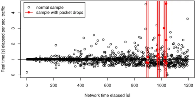
Figure 1 shows the real-time (Y-axis) that elapses while Bro processes each second of network traffic (X-axis). The vertical lines denote times at which the packet capture facility (libpcap) reports drops; the corresponding CPU samples are shown with afilled circle.

The NIDS can avoid drops as long as the number of processing outliers remains small—more precisely, as long as they can be compensated by buffering of captured packets. For example, the 20MB buffer used in our evaluations enabled us to process an extreme outlier—requiring 2.5 s for one real-time second worth of network traffic— without packet drops. Accordingly, we find that the first packet drop occurs only after a spike in processing real time of more than 4s. Closer inspection shows that the loss does not occur immediately during processing the “expensive” traffic but rather six network seconds later. It is only at that point that the buffer is completely full and

0 200 400 600 800 1000 1200 0 1 2 3 4

Network time elapsed [s]

Real time [s] elapsed per sec. traffic

normal sample sample with packet drops

Fig. 1.Relation between elapsed real-time and packet drops.

thelag(i.e., how far the NIDS is behind in its processing) exceeds 5.5s. Such a large amount of buffering thus makes it difficult to predict the occurrence of drops and their likely magnitude:(i)the buffer can generally absorb single outliers, and(ii)the buffer capacity (in seconds) depends on the traffic volume yet to come. But clearly we desire to keep the lag small.

Memory Exhaustion. When a stateful NIDS completely consumes the memory avail-able to it, it can no longer effectively operate, as it cannot store additional state. It can, however, try to reclaim memory by expiring existing state. The challenges here are (i)how to recognize that an exhaustion condition is approaching prior to its actual on-set,(ii)in the face of often complex internal data structures [3], and then(iii)locating apt state to expire that minimizes the ability for attackers to leverage the expiration for evading detection.

One simple approach for limiting memory consumption imposes a limit on the size of each internal data structure. Snort [8], for example, allows the user to specify a maximum number of concurrent connections for its TCP preprocessor. If this limit is reached, Snort randomly picks some connections and flushes their state to free up mem-ory. Similarly, Snort addresses the issue of variable stream reassembly size by providing an option to limit the total number of bytes in the reassembler. Bro on the other hand does not provide a mechanism to limit the size of data structures to a fixed size; its state management instead relies on timeouts, which can be set on a per-data structure basis, and with respect to when state was first created, or last read or updated. However, these do not provide a guarantee that Bro can avoid memory exhaustion, and thus it can crash in the worst case. Bro does however include extensive internal memory instrumenta-tion [3] to understand its consumpinstrumenta-tion, which we leverage for our measurements.

Memory consumption and processing lag can become coupled in two different ways. First, large data structures can take increasingly longer to search as they grow in size, increasing the processing burden. Second, in systems that provide more vir-tual memory than physical memory, consuming the entire physical memory does not crash the system but instead degrades its performance due to increased paging activity. In the worst case, such systems can thrash, which can enormously diminish real-time performance.

3 Modeling NIDS Resource Usage

In this section we consider the high-level components that determine the resource usage of a NIDS. We first discuss the rationale that leads to our framing of the components, and then sketch our resulting distillation. The next section proceeds to evaluate the framework against the Bro NIDS.

3.1 The Structure of NIDS Processing

Fundamental to a NIDS’s operation is tracking communication between multiple net-work endpoints. All major NIDS’s today operate in astatefulfashion, decoding network communication according to the protocols used, and to a degree mirroring the state maintained by the communication endpoints. This state naturally grows proportional to the number of active connections1_{, and implementations of stateful approaches are} nat-urally aligned with the network protocol stack. To reliably ascertain the semantics of an application-layer protocol, the system first processes the network and transport layers of the communication. For example, for HTTP the NIDS first parses the IP header (to ver-ify checksums, extract addresses, determine transport protocol, and so on) and the TCP header (update the TCP state machine, checksum the payload), and then reassembles the TCP byte stream, before it can finally parse the HTTP protocol.

A primary characteristic of the network protocol stack is its extensive use of en-capsulation: individual layers are independent of each other; while their input/output is connected, there ideally is no exchange of state between layers. Accordingly, for a NIDS structured along these lines its protocol-analyzing components can likewise operate independently. In particular, it is plausible to assume that the total resource consumption, in terms of CPU and memory usage, is the sum of the demands of the individual components. This observation forms a basis for our estimation methodology. In operation, a NIDS’s resource usage primarily depends on the characteristics of the network traffic it analyzes; it spends its CPU cycles almost exclusively on analyzing input traffic, and requires memory to store results as it proceeds. In general, network packets provide the only sustained stream of input during operation, and resource usage therefore should directly reflect the volume and content of the analyzed packets.2

We now hypothesize that for each component of a NIDS that analyzes a particular facet or layer of network activity—which we term an analyzer—the relationship be-tween input traffic and the analyzer’s resource demands is linear. Lett0 be the time when NIDS operation begins, and Pt the number of input packets seen up to time t ≥ t0. Furthermore, letCt be thetotalnumber of transport-layer connections seen up to timet, andct the number of connectionscurrently activeat time t. Then we argue: Network-layer analyzers operate strictly on a per-packet basis, and so should requireO(Pt)CPU time, and rarely store state. (One exception concerns reassembly of IP fragments; however, in our experience the memory required for this is negligi-ble even in large networks.)Transport-layeranalyzers also operate packet-wise. Thus,

1_{For UDP and ICMP we assume flow-like definitions, similar to how NetFlow abstracts packets.} 2_{In this work, we focus on stand-alone NIDSs that analyze traffic and directly report alerts. In} more complex setups (e.g., with distributed architectures) resource consumption may depend on other sources of input as well.

their amortized CPU usage will scale asO(Pt). However, transport-layer analyzers can require significant memory, such as tracking TCP sequence numbers, connection states, and byte streams. These analyzers therefore will employ data structures to store all cur-rently active connections, requiringO(max(ct))memory. For stream-based protocols, the transport-layer performs payload reassembly, which requires memory that scales withO(max(ct·mt)), wheremtrepresents the largest chunk of unacknowledged data on any active connection at timet(cf. [1]). Finally,application-layeranalyzers exam-ine the payload data as reconstructed by the transport layer. Thus, their CPU time scales proportional to the number of connections, and depends on how much of the payload the analyzer examines. (For example, an HTTP analyzer might only extract the URL in client requests, and skip analysis of the much larger server reply.) The total size of the connection clearly establishes an upper limit. Accordingly, the state requirements for application analyzers will depend on the application protocol and will be kept on a per-connection basis, so will scale proportional to the protocolmix(how prevalent the application is in the traffic stream) and the number of connectionsct.

In addition to protocol analyzers, a NIDS may performinter-connectioncorrelation. For example, a scan detector might count connections per source IP address, or an FTP session analyzer might follow the association between FTP client directives and subse-quent data-transfer connections. In general, the resource usage of such analyzers can be harder to predict, as it will depend on specifics of the analysis (e.g., the scan detector above requiresO(Ct)CPU and memory if it does not expire any state, while the FTP session analyzer only requires CPU and memory in proportion to the number of FTP client connections). However, in our experience it is rare that such analyzers exceed CPU or memory demands ofO(Ct), since such analysis quickly becomes intractable on any high-volume link. Moreover, while it is possible that such inter-connection an-alyzer may depend on the results of other anan-alyzers, we find that such anan-alyzers tend to be well modular and decoupled (e.g., the scan detector needs the same amount of memory independent of whether the NIDS performs HTTP URL extraction or enables FTP session-tracking).

3.2 Principle Contributors to Resource Usage

Overall, it appears reasonable to assume that for a typical analyzer, resource usage is(i) linear with either the number of input packets or the number of connections it processes, and(ii)independent of other analyzers. In this light, we can frame two main contributors to the resource usage of a NIDS:

1. The specific analyzers enabled by the operator for the system’s analysis. That these contribute to resource usage is obvious, but the key point we want to make is that most NIDSs provide options to enable/disable certain analyzers in order to trade off resource requirements. Yet NIDSs give the operators almost no concrete guidance regarding the trade-offs, so it can be extremely hard to predict the performance of a NIDS when enabling different sets of analyzers. This difficulty motivated us to build our toolnidsconf(per§5.2) that provides an understanding of resource usage trade-offs to support configuration decisions.

2. The trafficmixof the input stream—i.e., the prevalence of different types of appli-cation sessions—as this affects the number of connections examined by each type of analyzers.

The above reasoning need not hold universally. However, we examined the archi-tecture of two popular open source NIDS, Snort and Bro, and found that their resource consumption indeed appears consistent with the model discussed above. We hypothe-size that we can characterize most operational NIDSs in this fashion, and thus they will lend themselves well to the kind of performance prediction we outline in§5. To support our claims, we now explore the resource usage of the Bro NIDS in more depth.

4 Example NIDS Resource Usage

To assess our approach of modeling a NIDS’s resource demands as the sum of the requirements of its individual analyzers, and scaling linearly with the number of appli-cation sessions, we now examine an example NIDS. Among the two predominant open-source NIDSs, Snort and Bro, we chose to examine Bro for two reasons:(i)Bro pro-vides a superset of Snort’s functionality, since it includes both a signature-matching en-gine and an application-analysis scripting language; and(ii)it provides extensive, fine-grained instrumentation of its internal resource consumption; see [3] for the specifics of how the system measures CPU and memory consumption in real-time. Snort does not provide similar capabilities. For our examination we have to delve into details of the Bro system, and we note that some of the specifics of our modeling are necessarily tied to Bro’s implementation. While this is unavoidable, as discussed above we believe that similar results will hold for Snort and other modern NIDSs.

For our analysis we captured a 24-hour full trace at the border router of the M¨unchener Wissenschaftsnetz (MWN). This facility provides 10 Gbps upstream ca-pacity to roughly 50,000 hosts at two major universities, along with additional research institutes, totaling 2-4 TB a day. To avoid packet drops, we captured the trace with a high-performance Endace DAG card. The trace encompasses 3.2 TB of data in 6.3 bil-lion packets and 137 milbil-lion connections. 76% of all packets are TCP. In the remainder of this paper, we refer to this trace asMWN-full.

4.1 Decomposition of Resource Usage

We first assess our hypothesis that we can consider the resource consumption of the NIDS’s analyzers as independent of one another. We then check if resource usage gen-erally scales linearly with the number of connections on the monitored network link.

Independence of Analyzer Resource Usage. For our analysis we use Bro version 1.1, focusing on 13 analyzers: finger,frag,ftp, http-request,ident, irc,login, pop3, portmapper,smtp,ssh,ssl, andtftp. To keep the analyzed data volume tractable, we use a 20-minute, TCP-only excerpt ofMWN-full, which we refer to asTrace-20m,

We run 15 different experiments. First, we establish a base case (BROBASE), which only performs generic connection processing. In this configuration, Bro only analyzes

0.4 0.6 0.8 1.0 1.2 1.4 1.6 0.4 0.6 0.8 1.0 1.2 1.4 1.6

CPU time [s], all analyzers loaded

CPU time [s], all analyzers summed up

sum of analyzer workloads sum of normalized analyzer workloads no error

+0.2s absolute error

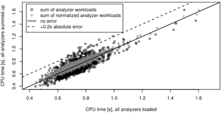
Fig. 2.Scatter plot of accumulated CPU usages vs. measured CPU usage.

connection control packets, i.e., all packets with any of the TCP flags SYN, FIN or RST set. This suffices for generating one-line summaries of each TCP connection in the trace. BROBASE thus reflects a minimal level of still-meaningful analysis. Next, we run a fully loaded analysis, BROALL, which enables all analyzers listed above, and by far exceeds the available resources. Finally, we perform 13 additional runs where we enable a single one of the analyzers on top of the BROBASEconfiguration. For each test, Bro is supplied with a trace prefiltered for the packets the configuration examines. This mimics live operation, where this filtering is usually done in the kernel and therefore not accounted to the Bro process.

We start with examining CPU usage. For each of the 13 runs using BROBASEplus one additional analyzer, we calculate the contribution of the analyzer as the difference in CPU usage between the run and that for the BROBASEconfiguration. We then form an estimate of the time of the BROALLconfiguration as the sum of the contributions of the individual analyzers plus the usage of the BROBASEconfiguration. We term this estimate BROAGG.

Figure 2 shows a scatter plot of the measured CPU times. Each point in the plot corresponds to the CPU time required for one second of network input. The circles reflect BROAGG(Y-axis) versus BROALL(X-axis), with five samples between 1.7s and 2.6s omitted from the plot for legibility. We observe that there is quite some variance in the matching of the samples: The mean relative error is 9.2% (median 8.6%) and for some samples the absolute error of BROAGG’s CPU time exceeds 0.2s (20% CPU load). There is also a systematic bias towards slight underestimation by BROAGG, with about 64% of its one-second intervals being somewhat lower than the value measured during that interval for BROALL.

To understand the origin of these differences, we examine the relative contribution of the individual analyzers. We find that there are a number of analyzers that do not add significantly to the workload, primarily due to those that examine connections that are not prevalent in the analyzed network trace (e.g.,finger). The resource consumption with these analyzers enabled is very close to that for plain BROBASE. Furthermore, due to the imprecision of the operating system’s resource accounting, two measurements of the same workload are never exactly the same; in fact, when running the BROBASE configuration ten times, the per-second samples differ by MR = 18msec on

aver-age. This means that if an analyzer contributes very little workload, we cannot soundly distinguish its contribution to CPU usage from simple measurement variation. The fluc-tuations of all individual runs with just one additional analyzer may well accumulate to the total variation seen in Figure 2.

To compensate for these measurement artifacts, we introduce a normalization of CPU times, as follows. For each single-analyzer configuration, we first calculate the dif-ferences of all its CPU samples with respect to the corresponding samples of BROBASE. If the mean of these differences is less than the previously measured value ofMRthen we instead predict its load based on aggregation across 10-second bins rather than 1-second bins. The ’+’ symbols in Figure 2 show the result: we both reduce overall fluc-tuation considerably, and no sample of BROAGGexceeds BROALLby more than 0.2s. The mean relative error drops to 3.5% (median 2.8%), indicating a good match. As in the non-normalized measurements, for most samples (71%) the CPU usage is extrapo-lated to slightly lower values than in the actual BROALLmeasurement. The key point is we achieve these gains solely by aggregating the analyzers that introduce very light additional processing. Thus, we conclude that(i)these account for the majority of the inaccuracy,(ii)correcting them via normalization does not diminish the soundness of the prediction, and(iii)otherwise, analyzer CPU times do in fact sum as expected.

Turning to memory usage, we use the same approach for assessing the additivity of the analyzers. We compute the difference in memory allocation between the instance with the additional analyzer enabled versus that of BROBASE. As expected, summing these differences and adding the memory consumption of BROBASE yields 465 MB, closely matching the memory usage of BROALL(461 MB).

Overall, we conclude that we can indeed consider the resource consumption of the analyzers as independent of one another.

Linear Scaling with Number of Connections. We now assess our second hypothesis: that a NIDS resource consumption scales linearly with the number of processed connec-tions. For this evaluation, we run Bro with identical configurations on traces that differ mainly in the number of connections that they contain at any given time. To construct such traces, we randomly subsample an input trace using per-connection sampling with different sampling factors, run Bro on the subtrace, and compare the resulting resource usage in terms of both CPU and memory. To then extrapolate the resource usage on the full trace, we multiply by the sample factor.

To sample a trace with a sample factorP, we hash the IP addresses and port num-bers of each packet into a range [0;P −1]and pick all connections that fall into a particular bucket. We choose a prime for the sample factor to ensure we avoid aliasing; this approach distributes connections across all buckets in a close to uniform fashion as shown in [11]. For our analysis we sampledTrace-20mwith sampling factorsP = 7

(resulting in STRACE7) andP = 31(resulting in STRACE31).

CPU Usage. Figure 3 shows a scatter plot of the CPU times for BROBASE on

Trace-20mwithout sampling, vs. extrapolating BROBASEon STRACE7 (circles) and

STRACE31 (triangles). We notice that in general the extrapolations match well, but are a bit low (the mean is 0.02 sec lower). Unsurprisingly, the fluctuation in the deviation

0.2 0.3 0.4 0.5

0.2

0.3

0.4

0.5

user time for analyzing unsampled trace

user time sampled traces

sampling factor 7 sampling factor 31

Fig. 3.Scatter plot of BROBASEconfiguration on sampled traces vs. non-sampled trace.

0.5 1.0 1.5 2.0 2.5

1

2

3

4

Quantile values w/o connection sampling

Quantile values w/ conn. sampling

80% 95%

sampling factor 7 sampling factor 11 sampling factor 17 sampling factor 31

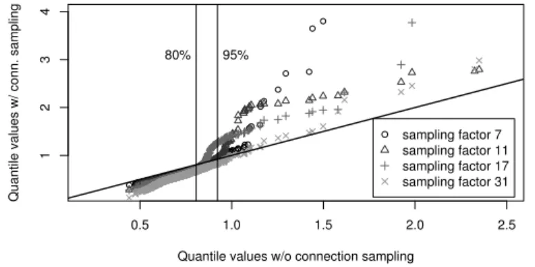
Fig. 4.QQ plot of analyzer workload without sampling vs. with different sampling factors.

from the originally measured values grows with the sampling factor (further measure-ments not included in Figure 3 with sampling factors between 7 and 31 confirm this).

Naturally, the measured CPU times are very small if only a few connections are analyzed. For example, in the unsampled trace Bro consumes on average 370 msec for one second of network traffic when analyzing all the connections. With a sampling factor of 31, we would expect consumption to drop to370/31 = 12 msec, at which point we are at the edge of the OS’s accounting precision. In fact, however, we find that extrapolation still works fairly well: for sample factor 31, the median of the extrapolated measurements is only 28 msec lower than the median of the measurements for the full trace. We have verified that similar observations hold for other segments ofMWN-full, as well as for other traces.

Next we check if this finding still holds for more complex configurations. To this end, the QQ-plot in Figure 4 compares the distribution of CPU times for BROALL(i.e., 13 additional analyzers) on the fullTrace-20m(X-axis) vs. sub-sampled traces (Y-axis, with sample factors of 7, 11, 17, and 31). Overall, the majority of the samples match fairly well, though with a bias for smaller values towards underestimation (left of the 80th percentile line), and with unstable upper quantiles (usually overestimates).

Sampling factor 1 7 11 17 31

Memory ratio 1 7.0 11.0 16.6 30.7

Sampling factor 1 7 11 17 31

Memory ratio 1 3.64 4.87 6.30 9.34

Table 1.Memory scaling factors: 10 BROBASEruns (left) / 10 BROALLruns (right).

Memory Usage. Turning to memory consumption, for each sampling factor we con-ducted 10 runs with BROBASEonTrace-20m, measuring the maximum consumption figures on the sampled traces as reported by the OS.3_{Table 1 (left) shows the ratio} be-tween the memory consumption on the entire trace versus that for the sampled traces. Ideally, this figure would match the sampling factor, since then we would extrapolate perfectly from the sample. We see that in general the ratio is close, with a bias towards being a bit low. From this we conclude that for BROBASE, predicting memory use from a sampled trace will result in fairly accurate, though sometimes slightly high, estimates. As discussed in Section 3, we would not expect memory usage of application-layer analyzers to always scale linearly with the number of connections, since some analyzers accumulate state not on a per-connection basis but rather according to somegrouping of the connections (e.g., Bro’s HTTP analyzer groups connections into “sessions”). In such cases the memory estimate we get by scaling with the connection sample factor can be a (potentially significant) overestimation. This effect is visible in Table 1 (right), which shows the same sort of analysis as above but now for BROALL. We see that the extrapolation factors can be off by more than a factor of three. By running each ana-lyzer separately, we identified the culprits: both the HTTP and SSL anaana-lyzers associate their state per session, rather than per connection. However, we note that at least the required memory neverexceedsthe prediction, and thus we can use the prediction as a conservative upper bound.

In summary, we find that both CPU and memory usage can generally be predicted well with a model linear in the number of connections. We need to keep in mind how-ever that it can overestimate the memory demand for some analyzers.

5 Resource Prediction

After confirming that we can often factor NIDS resource usage components with per-analyzer and per-connection scaling, we now employ these observations to derive sug-gestions of reasonable configurations for operating in a specific network environment.

We start by devising a methodology for finding a suitable configuration based on a snapshot of an environment’s network traffic. Then we turn to estimating the long-termperformance of such a configuration given a coarser-grained summary of the net-work traffic that contains the time-of-day and day-of-week effects. The latter is crucial, as traffic characteristics, and therefore resource consumption, can change significantly over time.

3_{As in the case of CPU usage, we find inherent fluctuation in memory usage as well: running} instances under identical conditions exhibits some noticeable, though not huge, variation.

5.1 From Traffic Snapshots to Configurations

In this section we consider the degree to which we can analyze a short sample trace from a given environment in order to identify suitable NIDS configurations, in terms of maximizing the NIDS’s analysis while leaving enough “head room” to avoid exhausting its resources. More generally, we wish to enable the network operator to make informed decisions about the prioritization of different types of analysis. Alternatively, we can help the operator decide whether to upgrade the machine if the available resources do not allow the NIDS to perform the desired analysis.

We stress that due to the variability inherent in network traffic, as well as the mea-surement limitations discussed in §4, no methodology can aim to suggest an optimal configuration. However, automating the process of exploring the myriad configuration options of a NIDS provides a significant step forward compared to having to assess different configurations in a time-consuming, trial-and-error fashion.

Capturing an Appropriate Trace. Our approach assumes access to a packet trace from the relevant network with a duration of some tens of minutes. We refer to this as themain analysis trace. At this stage, we assume the trace is “representative” of the busiest period for the environment under investigation. Later in this section we explore this issue more broadly to generalize our results.

Ideally, one uses afullpacket trace with all packets that crossed the link during the sample interval. However, even for medium-sized networks this often will not be feasi-ble due to disk capacity and time constraints: a 20-minute recording of a link transfer-ring 400 Mbit/s results in a trace of roughly 60 GB; running a systematic analysis on the resulting trace as described below would be extremely time consuming. In addition, full packet capture at these sorts of rates can turn out to be a major challenge on typical commodity hardware [9].

We therefore leverage our finding that in general we can decompose resource usage on a per-connection basis and take advantage of the connection sampling methodology discussed in Section 4. Given a disk space budget as input, we first estimate the link’s usage via a simple libpcap application to determine a suitable sampling factor, which we then use to capture an accordingly sampled trace. We can perform the sampling itself using an appropriate kernel packet filter [2], so it executes quite efficiently and imposes minimal performance stress on the monitoring system.

Using this trace as input, we then can scale our results according to the sample fac-tor, as discussed in§4, while keeping in mind the most significant source of error in this process, which is a tendency to overestimate memory consumption when considering a wide range of application analyzers.

Finding Appropriate Configurations. We now leverage our observation that we can decompose resource usage per analyzer to determine analysis combinations that do not overload the system when analyzing a traffic mix and volume similar to that extrapo-lated from the captured analysis trace. Based on our analysis of the NIDS resource us-age contributors (§3.2) and its verification (§4), our approach is straight-forward. First we derive a baseline of CPU and memory usage by running the NIDS on the sampled

trace using a minimal configuration. Then, for each potentially interesting analyzer, we measure its additional resource consumption by individually adding it to the mini-mal configuration. We then calculate which combinations of analyzers result in feasible CPU and memory loads.

The main challenge for determining a suitable level ofCPU usage is to find the right trade-off between a good detection rate (requiring a high average CPU load) and leaving sufficient head-room for short-term processing spikes. The higher the load bud-get, the more detailed the analysis; however, if we leave only minimal head-room then the system will likely incur packet drops when network traffic deviates from the typical load, which, due to the long-range dependent nature of the traffic [12] will doubtlessly happen. Which trade-off to use is apolicy decisionmade by the operator of the NIDS, and depends on both the network environment and the site’s monitoring priorities. Ac-cordingly, we assume the operator specifies a target CPU loadctogether with a quantile qspecifying the percentage of time the load should remain belowc. With, for example, c= 90%andq= 95%, the operator asks our tool to find a configuration that keeps the

CPU load below 90% for 95% of all CPU samples taken when analyzing the trace. Two issues complicate the determination of a suitable level ofmemoryusage. First, some analyzers that we cannot (reasonably) disable may consume significant amounts of memory, such as TCP connection management as a precursor to application-level analysis for TCP-based services. Thus, the option is not whether to enable these ana-lyzers, but rather how toparameterizethem (e.g., in terms of setting timeouts). Second, as pointed out in§4, the memory requirements of some analyzers do not scale directly with the number of connections, rendering their memory consumption harder to predict. Regarding the former, parameterization of analyzers, previous work has found that connection-level timeouts are a primary contributor to a NIDS’s memory consump-tion [3]. Therefore, our first goal is to derive suitable timeout values given the connec-tion arrival rate in the trace. The main insight is that the NIDS needs to store different amounts of state for different connection types. We can group TCP connections into three classes:(i)failed connection attempts;(ii)fully established and then terminated connections; and(iii)established but not yet terminated connections. For example, the Bro NIDS (and likely other NIDSs as well) uses different timeouts and data structures for the different classes [3], and accordingly we can examine each class separately to determine the corresponding memory usage. To predict the effect of the individual timeouts, we assume a constant arrival rate for new connections of each class, which is reasonable given the short duration of the trace. In addition, we assume that the memory required for connections within a class is roughly the same. (We have verified this for Bro.) This then enables us to estimate appropriate timeouts for a given memory budget. To address the second problem, analyzer memory usage which does not scale lin-early with the sampling factor, we can identify these cases by “subsampling” the main trace further, using for example an additional sampling factor of 3. Then, for each an-alyzer, we determine the total memory consumption of the NIDS running on the sub-sampled trace and multiply this by the subsampling factor. If doing so yields approx-imately the memory consumption of the NIDS running the same configuration on the main trace, then the analyzer’s memory consumption does indeed scale linearly with the sampling factor. If not, then we are able to flag that analysis as difficult to extrapolate.

5.2 A Tool for Deriving NIDS Configurations

We implemented an automatic configuration tool,nidsconf, for the Bro NIDS based on the approach discussed above. Using a sampled trace file, it determines a set of Bro configurations, including sets of feasible analyzers and suitable connection timeouts. These configurations enable Bro to process the network’s traffic within user-defined limits for CPU and memory.

We assessednidsconfin the MWN environment on a workday afternoon with a disk space budget for the sampled trace of 5 GB; a CPU limit ofc = 80%forq = 90%of all samples; a memory budget of 500 MB for connection state; and a list of 13 different analyzers to potentially activate (mostly the same as listed previously, but also includinghttp-replywhich examines server-side HTTP traffic).

Computed over a 10-second window, the peak bandwidth observed on the link was 695 Mbps. A 20-minute full-packet trace would therefore have required approximately 100 GB of data. Consequently,nidsconfinferred a connection sampling factor of 23 as necessary to stay within the disk budget (the next larger prime above the desired sam-pling factor of 21). The connection-sampled trace that the tool subsequently captured consumed almost exactly 5 GB of disk space.nidsconfthen concluded that even by itself, full HTTP request/reply analysis would exceed the givencandqconstraints. Therefore it decided to disable server-side HTTP analysis. Even without this, the com-bination of all other analyzers still exceeded the constraints. Therefore, the user was asked to chose one to disable, for which we selectedhttp-request. Doing so turned out to suffice. In terms of memory consumption,nidsconfdetermined that the amount of state stored by three analyzers (HTTP, SSL, and the scan detector) did not scale linearly with the number of connections, and therefore could not be predicted correctly. Still, the tool determined suitable timeouts for connection state (873 secs for unanswered connection attempts, and 1653 secs for inactive connections).

Due to the complexity of the Bro system, there are quite a few subtleties involved in the process of automatically generating a configuration. Due to limited space, here we only outline some of them, and refer to [2] for details. One technical complication is that not all parts of Bro are sufficiently instrumented to report their resource usage. Bro’s scripting language poses a more fundamental problem: a user is free to write script-level analyzers that consume CPU or memory in unpredictable ways (e.g., not tied to connections). Another challenge arises due to individual connections that require specific, resource-intensive analysis. As these are non-representative connections any sampling-based scheme must either identify such outliers, or possibly suggest overly conservative configurations. Despite these challenges, however,nidsconfprovides a depth of insight into configuration trade-offs well beyond what an operator otherwise can draw upon.

5.3 From Flow Logs to Long-Term Prediction

Now that we can identify configurations appropriate for a short, detailed packet-level trace, we turn to estimating thelong-termperformance of such a configuration. Such extrapolation is crucial before running a NIDS operationally, as network traffic tends to exhibit strong time-of-day and day-of-week effects. Thus, a configuration suitable for a

short snapshot may still overload the system at another time, or unnecessarily forsake some types of analysis during less busy times.

For this purpose we require long-term, coarser-grained logs of connection informa-tion as an abstracinforma-tion of the network’s traffic. Such logs can, for example, come from NetFlow data, or from traffic traces with tools such as tcpreduce [10], or perhaps the NIDS itself (Bro generates such summaries as part of its generic connection analysis). Such connection-level logs are much smaller than full packet traces (e.g.,1% of the volume), and thus easier to collect and handle. Indeed, some sites already gather them on a routine basis to facilitate traffic engineering or forensic analysis.

Methodology. Our methodology draws upon both the long-term connection log and the systematic measurements on a short-term, (sampled) full-packet trace as described above. We proceed in three steps: First, we group all connections (in both the log and the packet trace) into classes, such that the NIDS resource usage scales linearly with the class size. Second, for different configurations, we measure the resources used by each class based on the packet trace. In the last step, we project the resource usage over the duration of the connection log by scaling each class according to the number of such connections present in the connection log.

In the simplest case, the overall resource usage scales linearly with thetotalnumber of connections processed (for example, this holds for TCP-level connection processing without any additional analyzers). Then we have only one class of connections and can project the CPU time for any specific time during the connection log proportionally: if in the packet trace the analysis ofNconnections takesPseconds of CPU time, we esti-mate that the NIDS performing the same analysis forMconnections uses P

NMseconds of CPU time. Similarly, if we know the memory required forIconcurrent connections at some timeT1for the packet trace, we can predict the memory consumption at time T2by determining the number of active connections atT2.

More complex configurations require more than one connection class. Therefore we next identify how to group connections depending on the workload they generate. Based on our observation that we can decompose a NIDS’s resource requirements into that of its analyzers (§3), along with our experience validating our approach for Bro (§4), we identified three dimensions for defining connection classes: duration, application-layer service, and final TCP state of the connection (e.g., whether it was correctly es-tablished). Duration is important for determining the number of active connections in memory at each point in time; service determines the analyzers in use; and the TCP state indicates whether application-layer analysis is performed.

As we will show, this choice of dimensions produces resource-consumption predic-tions with reasonable precision for Bro. We note, however, that for other NIDSs one might examine a different decomposition (e.g., data volume per connection may have a strong impact too). Even if so, we anticipate that a small number of connection classes will suffice to capture the principle components of a NIDS’s resource usage.

Predicting Long-Term Resource Use. We now show how to apply our methodology to predict the long-term resource usage of a NIDS, again using Bro as an example. We first aggregate the connection-level data into time-bins of lengthT, assigning attributes

local time

CPU time per second

0.0 0.5 1.0 1.5 2.0 2.5

Tue 14:00 Tue 18:00 Tue 22:00 Wed 2:00 Wed 6:00 Wed 10:00 measured CPU time

predicted CPU time

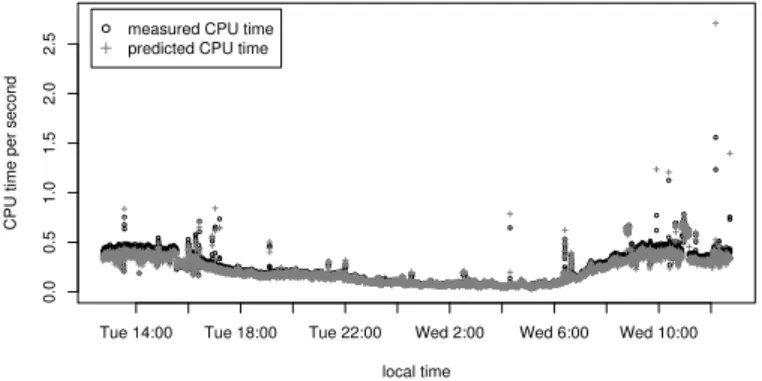
Fig. 5.Measured CPU time vs. predicted CPU time with BROBASE.

reflecting each of the dimensions: TCP state, service, and duration. We distinguish be-tween five TCP states (attempted, established, closed, half-closed, reset), and consider 40 services (one for each Bro application-layer analyzer, plus a few additional well-known service ports, plus the service “other”). We discretize a connection’s durationD by assigning it to a duration categoryC ← blog10Dc. Finally, for each time-bin we count the number of connections with the same attributes.

Simple CPU Time Projection. To illustrate how we then project performance, let us first consider a simple case: the BROBASE configuration. As we have seen (§4), for this configuration resource consumption directly scales with the total number of connections. In Figure 5 we plot the actual per-second CPU consumption exhibited by running BROBASE on the completeMWN-fulltrace (circles) versus the per-second consumption projected by using connection logs plus an independent 20-minute trace (crosses). We see that overall the predicted CPU time matches the variations in the measured CPU time quite closely. The prediction even correctly accounts for many of the outliers. However, in general the predicted times are somewhat lower than the measured ones with a mean error of -25 msec of CPU time per second, and a mean relative error of -9.0%.

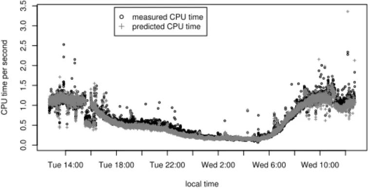
CPU Time Projection for Complex Configurations. Let us now turn to predicting performance for more complex configurations. We examine BROALL−, the BROALL

configuration except withssldeactivated (since the analyzer occasionally crashes the examined version of Bro in this environment). In this case, we group the connections into several classes, as discussed above. To avoid introducing high-variance effects from minimal samples, we discard any connections belonging to a service that comprises less than 1% of the traffic. (See below for difficulties this can introduce.) We then predict overall CPU time by applying our projection first individually to each analyzer and for each combination of service and connection state, and then summing the predicted CPU times for the base configuration and the predicted additional CPU times for the individual analyzers.

local time

CPU time per second

0.0 0.5 1.0 1.5 2.0 2.5 3.0 3.5

Tue 14:00 Tue 18:00 Tue 22:00 Wed 2:00 Wed 6:00 Wed 10:00 measured CPU time

predicted CPU time

Fig. 6.Measured CPU time vs. predicted CPU time with BROALL−

Figure 6 shows the resulting predicted CPU times (crosses) and measured BROALL− CPU times (circles). Note that this configuration is infeasible for a live

set-ting, as the required CPU regularly exceeds the machine’s processing capacity. We see, however, that our prediction matches the measurement fairly well. However, we under-estimate some of the outliers with a mean error of -29 msec of CPU time and a mean relative error of -4.6%. Note that the mean relative error is smaller than for predicting BROBASEperformance since the absolute numbers of the measured samples are larger for the complex configuration.

Above we discussed how we only extrapolate CPU time for connections that con-tribute a significant portion (>1%) of the connections in our base measurement. Doing so can result in underestimation of CPU time when these connection types become more prominent. For example, during our experiments we found that SSH and Telnet connections did not occur frequently in the 20-minute trace on which the systematic measurements are performed. Yet the long-term connection log contains sudden surges of these connections (likely due to brute-force login attempts).nidsconfdetects such cases and reports a warning, but at this point it lacks sufficient data to predict the CPU time usage, since it does not have an adequate sample in the trace from which to work.

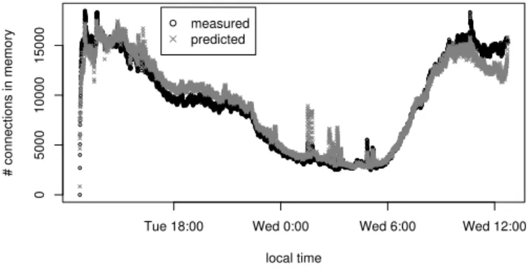
Memory Projection. Our approach for predictingmemoryconsumption is to derive the number of active connections per class at any given time in the connection log, and then extrapolate from this figure to the overall memory usage. However, Bro’s resource profiling is not currently capable of reporting precise per-connection memory usage for application-layer analyzers, so here we limit ourselves to predicting thenumberof TCP connections in memory, rather than the actual memory consumption. To do so, we draw upon the dimensions of connectiondurationandstate. These two interplay directly since Bro keeps its per connection state for the lifetime of the connection plus a timeout that depends on the state. To determine the relevant timeout, we use the states discussed above (attempted, established, etc.), binning connections into time intervals of lengthT and then calculating their aggregate memory requirements.

However, a problem with this binning approach arises due to connections with du-rations shorter than the bin size (since we use bin sizes on the order of tens of seconds,

local time # connections in memory 0 5000 10000 15000

Tue 18:00 Wed 0:00 Wed 6:00 Wed 12:00 measured

predicted

Fig. 7.Predicted number of established connections in memory forMWN-full.

this holds for the majority of connections). Within a bin, we cannot tell how many of these areconcurrentlyactive. Therefore, we refine our basic approach, as follows. We pick a random point in the base trace and compute the average numberNof short-lived connections per second occurring in the trace up to that point. We also measure the numberF of these short-lived connections instantaneously in memory at the arbitrary point. LetNibe the number of short-lived connections per second for each biniin the connection log. Assuming thatF is representative, we can then scaleNi/N byF to estimate the number of short-lived connections concurrently active in each bin.

Figure 7 shows the results of our prediction for the number of established connec-tions in memory (crosses) assuming Bro’s default inactivity timeout of 300s, along with the the actual number of in-memory connections when running onMWN-full(circles). We observe that the prediction matches the measurements well, with a mean relative er-ror of +5.0%. While not shown on the plot, we obtain similar prediction results for other classes of connections, e.g., unanswered connection attempts.

6 Related Work

Numerous studies in the literature investigate IDS detection quality, generally analyzing the trade-off between false positives and false negatives. Some studies [6, 4, 5] take steps towards analyzing how the detection quality and detection coverage depends on the cost of the IDS configuration and the attacks the network experiences. Gaffney and Ulvila [4] focus on the costs that result from erroneous detection, developing a model for finding a suitable trade-off between false positives and false negatives dependent on the cost of each type of failure. In contrast, Lee et al. [6, 5] focus on developing and implementing high-level cost models for operating an IDS, enabling dynamic adaptation of a NIDS’s configuration to suit the current system load. The models take as input both metrics of the benefits of a successful detection and (self-adapting) metrics reflecting the cost of the detection. Such metrics may be hard to define for large network environments, however. To adapt to the cost metrics, they monitor the performance of their prototype systems (Bro and Snort) using a coarse-grained instrumentation of packet counts per second. As was shown by Dreger et al. [3], this risks oversimplifying a complex NIDS.

While the basic idea of adapting NIDS configurations to system load is similar to ours, we focus on predicting resource usage of the NIDS depending on both the network traffic and the NIDS configuration.

In the area of general performance prediction and extrapolation of systems (not nec-essarily NIDSs), three categories of work exam(i)performance on different hardware platforms, (ii) distribution across multiple systems, and(iii) predicting system load. These studies relate to ours in the sense that we use similar techniques for program de-composition and for runtime extrapolation. We omit details of these here due to limited space, but refer the reader to [2] for a detailed discussion. In contrast to this body of work, our contributions are to predict performance forsoftreal-time systems, both at a fine-grained resolution (prediction of “head room” for avoiding packet drops) and over long time scales (coupling a short, detailed trace with coarse-grained logs to extrapo-late performance over hours or days), with an emphasis on memory and CPU trade-offs available to an operator in terms of depth of analysis versus limited resources.

7 Conclusion

In this work we set out to understand and predict the resource requirements of net-work intrusion detection systems. When initially installing such a system in a netnet-work environment, the operator often must grapple with a large number of options to tune trade-offs between detection rate versus CPU and memory consumption. The impact of such parameters often proves difficult to predict, as it potentially depends to a large degree on the internals of the NIDS’s implementation, as well as the specific charac-teristics of the target environment. Because of this, the installation of a NIDS often becomes a trial-and-error process that can consume weeks until finding a “sweet spot.” We have developed a methodology toautomaticallyderive NIDS configurations that maximize the systems’ detection capabilities while keeping the resource load fea-sible. Our approach leverages the modularity likely present in a NIDS: while complex systems, NIDSs tend to be structured as a set of subcomponents that work mostly inde-pendently in terms of their resource consumption. Therefore, to understand the system as a whole, we can decompose the NIDS into the main contributing components. As our analysis of the open-source Bro NIDS shows, the resource requirements of these subcomponents are often driven by relatively simple characteristics of their input, such as number of packets or number and types of connections.

Leveraging this observation, we built a tool that derives realistic configurations for Bro. Based on a short-term, full-packet trace coupled with a longer-term, flow-level trace—both recorded in the target environment—the tool first models the resource usage of the individual subcomponents of the NIDS. It then simulates different configurations by adding together the contributions of the relevant subcomponents to predict configu-rations whose execution will remain within the limits of the resources specified by the operator. The operator can then choose among the feasible configurations according to the priorities established for the monitoring environment. While no automatically gen-erated configuration can be optimal, these provide a sound starting point, with promise to significantly reduce the traditional trial-and-error NIDS installation cycle.

8 Acknowledgments

We would like to thank Christian Kreibich for his feedback and the fruitful discussions that greatly helped to improve this work. We would also like to thank the Leibnitz-Rechenzentrum M¨unchen. This work was supported by a grant from the Bavaria Cal-ifornia Technology Center, and by the US National Science Foundation under awards STI-0334088, NSF-0433702, and ITR/ANI-0205519, for which we are grateful. Any opinions, findings, conclusions or recommendations expressed in this material are those of the authors or originators and do not necessarily reflect the views of the National Sci-ence Foundation.

References

1. S. Dharmapurikar and V. Paxson. Robust TCP Stream Reassembly In the Presence of Ad-versaries. InProc. USENIX Security Symposium, 2005.

2. H. Dreger. Operational Network Intrusion Detection: Resource-Analysis Tradeoffs. PhD

thesis, TU M¨unchen, 2007. http://www.net.in.tum.de/˜hdreger/papers/

thesis_dreger.pdf.

3. H. Dreger, A. Feldmann, V. Paxson, and R. Sommer. Operational Experiences with High-Volume Network Intrusion Detection. InProc. ACM Conference on Computer and Commu-nications Security, 2004.

4. J. E. G. Jr and J. W. Ulvila. Evaluation of Intrusion Detectors: A Decision Theory Approach. InProc. IEEE Symposium on Security and Privacy, 2001.

5. W. Lee, J. B. Cabrera, A. Thomas, N. Balwalli, S. Saluja, and Y. Zhang. Performance Adap-tation in Real-Time Intrusion Detection Systems. InProc. Symposium on Recent Advances in Intrusion Detection, 2002.

6. W. Lee, W. Fan, M. Miller, S. J. Stolfo, and E. Zadok. Toward Cost-sensitive Modeling for Intrusion Detection and Response.Journal of Computer Security, 10(1-2):5–22, 2002. 7. V. Paxson. Bro: A System for Detecting Network Intruders in Real-Time. Computer

Net-works, 31(23–24):2435–2463, 1999.

8. M. Roesch. Snort: Lightweight Intrusion Detection for Networks. InProc. Systems Admin-istration Conference, 1999.

9. F. Schneider, J. Wallerich, and A. Feldmann. Packet Capture in 10-Gigabit Ethernet Envi-ronments Using Contemporary Commodity Hardware. InProc. Passive and Active Measure-ment Conference, 2007.

10. tcp-reduce.http://ita.ee.lbl.gov/html/contrib/tcp-reduce.html.

11. M. Vallentin, R. Sommer, J. Lee, C. Leres, V. Paxson, and B. Tierney. The NIDS Cluster: Scalable, Stateful Network Intrusion Detection on Commodity Hardware. InProc. Sympo-sium on Recent Advances in Intrusion Detection, 2007.

12. W. Willinger, M. S. Taqqu, R. Sherman, and D. V. Wilson. Self-Similarity Through High-Variability: Statistical Analysis of Ethernet LAN Traffic at the Source Level. IEEE/ACM Transactions on Networking, 5(1), 1997.