Anisha Ghosh,
Christian Julliard
, Alex, P. Taylor
What is the Consumption-CAPM missing?
An information-theoretic framework for the
analysis of asset pricing models
Article (Accepted version)
(Refereed)
Original citation: Ghosh, Anisha, Julliard, Christian and Taylor, Alex. P (2016) What is the Consumption-CAPM missing? An information-theoretic framework for the analysis of asset pricing models.The Review of Financial Studies . ISSN 0893-9454
DOI: 10.1093/rfs/hhw075
© 2016 The Authors
This version available at: http://eprints.lse.ac.uk/65131/ Available in LSE Research Online: December 2016
LSE has developed LSE Research Online so that users may access research output of the School. Copyright © and Moral Rights for the papers on this site are retained by the individual authors and/or other copyright owners. Users may download and/or print one copy of any article(s) in LSE Research Online to facilitate their private study or for non-commercial research. You may not engage in further distribution of the material or use it for any profit-making activities or any commercial gain. You may freely distribute the URL (http://eprints.lse.ac.uk) of the LSE Research Online website.
This document is the author’s final accepted version of the journal article. There may be differences between this version and the published version. You are advised to consult the publisher’s version if you wish to cite from it.
What is the Consumption-CAPM Missing?
An Information-Theoretic Framework for the Analysis of Asset
Pricing Models
∗Anisha Ghosh† Christian Julliard‡ Alex P. Taylor§
November 19, 2015
Abstract
We consider asset pricing models in which the SDF can be factorized into an observable component and a potentially unobservable one. Using a relative entropy minimization approach, we estimate non-parametrically the SDF and its components. Empirically, we find the SDF to have a business cycle pattern, and significant correlations with market crashes and the Fama-French factors. Moreover, we derive novel bounds for the SDF that are tighter, and have higher information content, than existing ones. We show that commonly used consumption-based SDFs: correlate poorly with the estimated one; require high risk aversion to satisfy the bounds; understate market crash risk.
Keywords: Pricing Kernel, Stochastic Discount Factor, Consumption Based Asset Pric-ing, Entropy Bounds.
JEL Classification Codes: G11, G12, G13, C52.
∗
We benefited from helpful comments from Mike Chernov, George Constantinides, Darrell Duffie, Bernard Dumas, Burton Hollifield, Ravi Jagannathan, Nobu Kiyotaki, Albert Marcet, Bryan Routledge, and seminar and conference participants at Carnegie Mellon University, the London School of Economics, INSEAD, Johns Hopkins University, 2011 Adam Smith Asset Pricing Conference, 2011 NBER Summer Institute, 2011 Society for Financial Econometrics Conference, 2011 CEPR ESSFM at Gerzensee, 2012 Annual Meeting of the American Finance Association. We are extremely thankful, for thoughtful and stimulating inputs, to Pietro Veronesi (the editor) and an anonymous referee. Christian Julliard thanks the Economic and Social Research Council (UK) [grant number: ES/K002309/1] for financial support.
†
Tepper School of Business, Carnegie Mellon University; [email protected]. ‡
Department of Finance, FMG and SRC, London School of Economics, and CEPR; [email protected]. §
I
Introduction
The absence of arbitrage opportunities implies the existence of a pricing kernel, also known as the stochastic discount factor (SDF), such that the equilibrium price of a traded security can be represented as the conditional expectation of the future pay-off discounted by the pricing kernel. The standard consumption-based asset pricing model, within the representative agent and time-separable power utility framework, identifies the pricing kernel as a simple parametric function of consumption growth. However, pricing kernels based on consumption growth alone cannot explain either the historically observed levels of returns, giving rise to the Equity Premium and Risk Free Rate Puzzles (e.g. Mehra and Prescott (1985), Weil (1989)), or the cross-sectional dispersion of returns between different classes of financial assets (e.g. Hansen and Sin-gleton (1983), Mankiw and Shapiro (1986), Breeden, Gibbons, and Litzenberger (1989), Campbell (1996)).1
Nevertheless, there is considerable empirical evidence that consumption risk does matter for explaining asset returns (e.g. Lettau and Ludvigson (2001a, 2001b), Parker and Julliard (2005), Hansen, Heaton, and Li (2008), Savov (2011)). Therefore, a bur-geoning literature has developed based on modifying the preferences of investors and/or the structure of the economy. In such models the resulting pricing kernel can be factor-ized into an observable component consisting of a parametric function of consumption growth, and a potentially unobservable, model-specific, component. Prominent exam-ples in this class include: the external habit model where the additional component consists of a function of the habit level (Campbell and Cochrane (1999); Menzly, San-tos, and Veronesi (2004)); the long run risks model based on recursive preferences where the additional component consists of the return on total wealth (Bansal and Yaron (2004)); and models with housing risk where the additional component con-sists of the growth in the expenditure share on non-housing consumption (Piazzesi, Schneider, and Tuzel (2007)). The additional, and potentially unobserved, compo-nent may also capture deviations from rational expectations (e.g. Brunnermeier and Julliard (2007)), models with robust control (e.g. Hansen and Sargent (2010)),
hetero-1Recently, Julliard and Ghosh (2012) show that pricing kernels based on consumption growth alone
cannot explain either the equity premium puzzle, or the cross-section of asset returns, even after taking into account the possibility of rare disasters.
geneous agents (e.g. Constantinides and Duffie (1996)), ambiguity aversion (e.g. Ulrich (2010)), as well as a liquidity factor arising from solvency constraints (e.g. Lustig and Nieuwerburgh (2005)).
In this paper, we propose a new methodology to analyze dynamic asset pricing models, such as those described above, for which the SDF can be factorized into an observable component and a potentially unobservable one. Our no-arbitrage approach allows us to: a) estimate non-parametrically from the data the time series of the unobserved pricing kernel under a set of asset pricing restrictions;b) construct entropy bounds to assess the empirical plausibility of candidate SDFs; c) estimate, given a fully observable pricing kernel, the minimum (in the information sense) adjustment of the SDF needed to correctly price asset returns. This methodology provides useful diagnostics tools for studying the ways in which various models might fail empirically, and allow us to characterize some properties that a successful model must satisfy.
First, we show that, given a set of asset returns and consumption data, a relative entropy minimization approach can be used to extract, non-parametrically, the time series of both the SDF and its unobservable component (if any). This methodology is equivalent to maximising the expected risk neutral likelihood under a set of no arbitrage restrictions. Moreover, given a fully observable pricing kernel, this procedure identifies theminimum amount of extra information that needs to be added to the SDF to enable it to price asset returns correctly. Along this dimension our paper is close in spirit to, and innovates upon, the long tradition of using asset (mostly options) prices to estimate the risk neutral probability measure (see e.g. Jackwerth and Rubinstein (1996), and Ait-Sahalia and Lo (1998)) and use this information to extract an implied pricing kernel (see e.g. Ait-Sahalia and Lo (2000), Rosenberg and Engle (2002), and Ross (2011)).
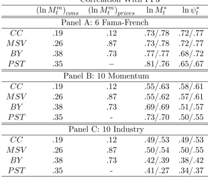
Empirically, our estimated time series for the unobservable pricing kernel is sub-stantially (but far from perfectly) correlated with the Fama and French (1993) factors, for a variety of sample frequencies and assets used in the estimation (even using only assets, like the industry and momentum portfolios, that are not well priced by the Fama-French factors).2 This suggests that our approach successfully identifies the
2
This correlation ranges from .45 to .81 when Fama-French portfolios are used in the estimation of the minimum entropy SDF, while it is reduced to the .43-.70 range when considering only Industry or
pricing kernel, and provides a rationalization of the empirical success of the Fama and French factors. The estimated SDF has a clear business cycle pattern but also shows significant and sharp reactions to stock market crashes (even if these crashes do not result in economy wide contractions). Moreover, we show that, while the SDFs of most of the equilibrium models tend to adequately account for business cycle risk, they nev-ertheless fail to show significant reactions to market crashes, and this hampers their ability to price asset returns – that is, all models seem to be missing a market crash risk component.
Second, we construct entropy bounds that restrict the admissible regions for the SDF and its unobservable component. Our results complement and improve upon the seminal work by Hansen and Jagannathan (1991), that provide minimum variance bounds for the SDF, and Hansen and Jagannathan (1997) (the so calledsecond Hansen-Jagannathan distance), that identifies the minimum variance (linear) modification of a candidate pricing kernel needed for it to be consistent with asset returns. The use of an entropy metric is also closely related to the works of Stutzer (1995, 1996), that first suggested to construct entropy bounds based on asset pricing restrictions, and Alvarez and Jermann (2005), who derive a lower bound for the volatility of the permanent component of investors’ marginal utility of wealth (see also Backus, Chernov, and Zin (2011), Bakshi and Chabi-Yo (2011) and Kitamura and Stutzer (2002)). We show that a second order approximation of the risk neutral entropy bounds (Q-bounds) have the canonical Hansen-Jagannathan bounds as a special case, but are generally tighter since they naturally impose the non negativity restriction on the pricing kernel. Using the multiplicative structure of the pricing kernel, we are able to provide novel bounds (M -bounds) that have higher information content, and are tighter, than both the Hansen and Jagannathan (1991) and the risk neutral entropy bounds. Moreover, our approach improves upon Alvarez and Jermann (2005) in that a decomposition of the pricing kernel into permanent and transitory components is not required (but is still possible), and we can accommodate an asset space of arbitrary dimension.
Our methodology can also be used to construct bounds (Ψ-bounds) for the poten-tially unobserved component of the pricing kernel. We show that for models in which
the pricing kernel is only a function of observable variables, the Ψ-bounds are the tight-est ones, and can be satisfied if and only if the model is actually able to correctly price assets. Moreover, when the pricing kernel is fully observable, our Ψ-bounds are closely related to the second Hansen-Jagannathan distance: HJ identify the minimum variance
linear adjustment, while our approach identifies the minimum entropy multiplicative
(or log-linear) adjustment, that would make a candidate pricing kernel consistent with observed asset returns. We show that the key difference between the two approaches is that the entropy one focuses not only on the second moment deviations, but also on all other higher moments. In an empirical example using stock return data we find that these higher moments play an important role driving about 22-26% of the entropy of the estimated pricing kernel.
Third, we demonstrate how our methodology provides useful diagnostic tools to assess the plausibility of some of the most well known consumption-based asset pricing models, and lends new insights about their empirical performance. For the standard time separable power utility model, we show that the pricing kernel satisfies the Hansen and Jagannathan (1991) bound for large values of the risk aversion coefficient, and the
Q and M bounds for even higher levels of risk aversion. However, the Ψ-bound is tighter and is not satisfied for any level of risk aversion. We show that these findings are robust to the use of the long run consumption risk measure of Parker and Julliard (2005), despite the fact that this measure of consumption risk is able to explain a sub-stantial share of the cross-sectional variation in asset returns with a small risk aversion coefficient. Considering more general models of dynamic economies, such as models with habit formation, long run risks in consumption growth, and complementarities in consumption, we find that the SDFs implied by all of thema) correlate poorly with the filtered SDF, b) require implausibly high levels of risk aversion to satisfy the entropy bounds, c) they all tend to understate market crash risk, in particular the risk asso-ciated with market crashes that do not result in recessions. Moreover, the empirical application illustrates that inference based on the entropy bounds delivers results that are much more stable, in evaluating the plausibility of a given model across different sets of assets and data frequencies, than the cross-sectionalR2 (that, instead, tends to
Compared to the previous literature, our nonparametric approach offers five main advantages: i) it can be used to extract information not only from options, as is com-mon in the literature, but also from any type of financial asset; ii) instead of relying exclusively on the information contained in financial data, it allow us to also exploit the information about the pricing kernel contained in the time series of aggregate con-sumption, thereby connecting our results to macro-finance modeling; iii) the relative entropy extraction of the SDF is akin to a nonparametric maximum likelihood proce-dure and provides an estimate of its time series; iv) the methodology has considerable generality, and may be applied to any model that delivers well-defined Euler equations and for which the SDF can be factorized into an observable component and an un-observable one (these include investment-based asset pricing models, and models with heterogenous agents, limited stock market participation, and fragile beliefs);v) it relies not only on the second moment of the pricing kernel, but also on all higher moments.
The remainder of the paper is organized as follows. Section II presents the information-theoretic methodology, the entropy bounds developed, and their properties. Section III uses the Consumption-CAPM with power utility as an illustrative example of the ap-plication of our methodology. Section IV applies the diagnostic tools developed in this paper to the analysis of more general models of dynamic economies. Section V con-cludes and discusses extensions. The Appendix contains proofs, additional empirical results and theoretical details, and a thorough data description.
II
Entropy and the Pricing Kernel
In the absence of arbitrage opportunities, there exists a strictly positive pricing kernel,
Mt+1, or stochastic discount factor (SDF), such that the equilibrium price, Pit, of any
assetidelivering a future payoff, Xit+1, is given by
Pit=Et[Mt+1Xit+1]. (1)
whereEt is the rational expectation operator conditional on the information available
at timet. For a broad class of models, the SDF can be factorized as follows
where m(θ, t) denotes the time t value of a known, strictly positive, function of ob-servable data and the parameter vector θ ∈ Θ ⊆ Rk with true value θ0, and ψt is a
potentially unobservable component. In the most common case, m(θ, t) is simply a function of consumption growth, i.e. m(θ, t) = m(θ,∆ct) where ∆ct ≡ logCCt−t1 and
Ctdenotes the time tconsumption flow.
Equations (1) and (2) imply that, for any set of tradable assets, the following vector of Euler equations must hold in equilibrium
0=E[m(θ, t)ψtRet]≡ Z
m(θ, t)ψtRetdP (3)
where E is the unconditional rational expectation operator,3 Ret ∈ RN is a vector
of excess returns on different tradable assets, and P is the unconditional physical probability measure. Under weak regularity conditions the above pricing restrictions for the SDF can be rewritten as
0= Z m(θ, t)ψ¯t ψR e tdP = Z m(θ, t)RetdΨ≡EΨ[m(θ, t)Ret]
where ¯x ≡E[xt], and ψψ¯t = dΨdP is the Radon-Nikodym derivative of Ψ with respect to
P. For the above change of measure to be legitimate, we need absolute continuity of the measures Ψ andP.
Therefore, given a set of consumption and asset returns data, for any θ, one can obtain a – non-parametric maximum likelihood – estimate of the Ψ probability measure as follows: Ψ∗(θ)≡arg min Ψ D(Ψ||P)≡arg min Ψ Z dΨ dP ln dΨ dPdP s.t. 0=E Ψ[m(θ, t)Re t] , (4)
where, for any two absolutely continuous probability measures A and B,D(A||B) :=
R
lndAdBdA ≡ R dA dBln
dA
dBdB denotes the relative entropy of A with respect to B, i.e.
the Kullback-Leibler Information Criterion (KLIC) divergence between the measures
3Our setting can accomodate departures from rational expectations as long as the objective and
subjective probability measures are absolutely continuos (i.e. as long as the two measures have the same zero probability sets). If agents had subjective beliefs of this type, equation (3) would still hold, withEdenoting rational expectations, butψtwould contain a change of measure element capturing the discrepancy between subjective beliefs and the rational expectations (see e.g. Hansen (2014, footnote 35)).
A and B (White (1982)). Note that D(A||B) is always non negative, and has a minimum at zero that is reached when A is identical to B. This divergence measures the additional information content ofArelative toB and, as pointed out by Robinson (1991), it is very sensitive to any deviation of one probability measure from another. Therefore, the above equation is a relative entropy minimization under the asset pricing restrictions coming from the Euler equations. That is, the minimization in equation (4) estimates the unknown measure Ψ as the one that adds the minimum amount of additional information needed for the pricing kernel to price assets.
To understand the information-theoretic interpretation of the estimator of Ψ, letF
be the set of all probability measures onRN+N 0
, whereN0 denotes the dimensionality of the observables inm(θ, t), and for each parameter vectorθ∈Θ, define the following set of probability measures
Ψ(θ)≡nψ∈F :Eψ[m(θ, t)Ret] =0 o
which are also absolutely continuous with respect to the physical measureP in equation (3). If the observable component of the SDF, m(θ, t), correctly prices assets at the given value ofθ, we have thatP ∈Ψ(θ), andP solves equation (4) delivering a KLIC value of 0. On the other hand, if m(θ, t) is not sufficient to price assets, P is not an element of Ψ(θ) and there is a positive KLIC distance D(Ψ||P) > 0 attained by the solution Ψ∗(θ). Thus, the estimation approach searches for a Ψ∗(θ) that adds the minimum amount of additional information needed for the pricing kernel to price asset returns.
The above approach can also be used, as first suggested by Stutzer (1995), to recover the risk neutral probability measure (Q) from the data as
Q∗ ≡arg min Q D(Q||P)≡arg min Q Z dQ dP ln dQ dPdP s.t. 0= Z RetdQ≡EQ[Ret] (5)
under the restriction thatQ and P are absolutely continuous.
The definition of relative entropy, or KLIC, implies that this discrepancy metric is not symmetric, that is generallyD(A||B)6=D(B||A) unless A and B are identical
(hence their divergence is always zero).4 This implies that for measuring the informa-tion divergence between Ψ andP, as well as betweenQand P, we can also invert the roles of Ψ and P in equation (4), and the roles ofQand P in equation (5), to recover Ψ andQas Ψ∗(θ)≡arg min Ψ D(P||Ψ)≡arg min Ψ Z lndP dΨdP s.t. 0=E Ψ[m(θ, t)Re t], (6) Q∗≡arg min Q D(P||Q)≡arg min Q Z lndP dQdP s.t. 0=E Q[Re t]. (7)
The divergence D(P||Ψ) can be thought of as the information loss from measure Ψ to measure P (and similarly for D(P||Q)). This alternative approach, once again, chooses Ψ and Q such that assets are priced correctly and such that the estimated probability measures are as close as possible (i.e. minimizing the information loss of moving from one measure to the other) to the physical probability measureP.
Note that the approaches in equations (4) and (6) identify {ψt}Tt=1 only up to a
positive scale constant. Nevertheless, this scaling constant can be recovered from the Euler equation for the risk free asset (if one is willing to assume that such an asset is observable).
But why should relative entropy minimization be an appropriate criterion for re-covering the unknown measures Ψ andQ? There are several reasons for this choice.
First, as formally shown in Appendix A.1, the KLIC minimizations in equations (4)-(7) are equivalent to maximizing the (expected)5 Q and Ψ non-parametric likelihood functions in an unbiased procedure for finding the pricing kernel or itsψt component.
Note that this is also the rationale behind the principle of maximum entropy (see e.g. Jaynes (1957a, 1957b)) in physical sciences and Bayesian probability that states that, subject to known testable constraints – the asset pricing Euler restrictions in our case – the probability distribution that best represent our knowledge is the one with maximum entropy, or minimum relative entropy in our notation.
Second, the use of relative entropy, due to the presence of the logarithm in the
4
Information theory provides an intuitive way of understanding the asymmetry of the KLIC:
D(A||B) can be thought of as the expected minimum amount of extra information bits necessary
to encode samples generated fromAwhen using a code based onB (rather than using a code based
on A). Hence generally D(A||B) 6= D(B||A) since the latter, by the same logic, is the expected
information gain necessary to encode a sample generated fromB using a code based onA.
5
objective functions in equations (4)-(7), naturally imposes the non negativity of the pricing kernel. This, for example, is not imposed in the identification of the minimum variance pricing kernel of Hansen and Jagannathan (1991).6
Third, our approach to uncover theψtcomponent of the pricing kernel satisfies the
Occam’s razor, or law of parsimony, since it adds theminimum amount of information
needed for the pricing kernel to price assets. This is due to the fact that the relative entropy is measured in units of information.
Fourth, it is straightforward to add conditioning information to construct a condi-tional version of the entropy bounds presented in the next Section: given a vector of conditioning variablesZt−1, one simply has to multiply (element by element) the
argu-ment of the integral constraints in equations (4), (5), (6) and (7) by the conditioning variables inZt−1.
Fifth, there is no ex-ante restriction on the number of assets that can be used in constructing ψt, and the approach can naturally handle assets with negative expected
rates of return (cf. Alvarez and Jermann (2005)).
Sixth, as implied by the work of Brown and Smith (1990), the use of entropy is desirable if we think that tail events are an important component of the risk measure.7 Finally, this approach is numerically simple when implemented via duality (see e.g. Csiszar (1975)). That is, when implementing the entropy minimization in equation (4) each element of the series {ψt}Tt=1 can be estimated, up to a positive constant scale
factor, as ψt∗(θ) = e λ(θ)0m(θ,t)Re t T X t=1 eλ(θ)0m(θ,t)Re t , ∀t (8)
whereλ(θ)∈RN is the solution to the following unconstrained convex problem
λ(θ)≡arg min λ 1 T T X t=1 eλ0m(θ,t)Ret, (9)
and this last expression is the dual formulation of the entropy minimization problem
6
Hansen and Jagannathan (1991) offer an alternative bound that imposes this restriction, but it is computationally cumbersome (the minimum variance portfolio is basically an option in this case). See also Hansen, Heaton, and Luttmer (1995).
7
Brown and Smith (1990) develop what they call “a Weak Law of Large Numbers for rare events,” that is they show that the empirical distribution that would be observed in a very large sample
in equation (4).
Similarly, the entropy minimization in equation (6) is solved by
ψt∗(θ) = 1
T(1 +λ(θ)0m(θ, t)Re t)
, ∀t (10)
whereλ(θ)∈RN is the solution to
λ(θ)≡arg min λ − T X t=1 log(1 +λ0m(θ, t)Ret), (11)
and this last expression is the dual formulation of the entropy minimization problem in equation (6).
Note also that the above duality results imply that the number of free parameters available in estimating{ψ}Tt=1 is equal to the dimension of (the Lagrange multiplier)λ
– that is, it is simply equal to the number of assets considered in the Euler equation. Moreover, since the λ(θ)’s in equations (9) and (11) are akin to Extremum Esti-mators (see e.g. Hayashi (2000, Ch. 7)), under standard regularity conditions (see e.g. Amemiya (1985, Theorem 4.1.3)), one can construct asymptotic confidence intervals for both {ψt}Tt=1 and the entropy bounds presented in the next Section.
To summarize, we estimate the ψt component of the SDF non-parametrically,
us-ing the relative entropy minimizus-ing procedures in equations (4) and (6). The estimate
{ψ∗t(θ)}Tt=1 is then multiplied with the observable component m(θ, t) to obtain the overall SDF, Mt∗ = m(θ, t)ψ∗t(θ). Since we have proposed two different relative en-tropy minimization approaches, we get two different estimates of the SDF given the data. Asymptotically, the two should be identical given the MLE property of these procedures, nevertheless in any finite sample they could potentially be very different. As shown in our empirical analysis, the two estimates are very close to each other, suggesting that their asymptotic behaviour is well approximated in our sample.
II.1 Entropy Bounds
Based on the relative entropy estimation of the pricing kernel and its component ψ
outlined in the previous Section, we now turn our attention to the derivation of a set of entropy bounds for the SDF, M, and its components.
Dynamic equilibrium asset pricing models identify the SDF as a parametric function of variables determined by the consumers’ preferences and the state variables driving the economy. A substantial research effort has been devoted to develop diagnostic methods to assess the empirical plausibility of candidate SDFs, as well as to provide guidance for the construction and testing of other – more realistic – asset pricing theories.
The seminal work by Hansen and Jagannathan (1991) identifies, in a model-free no-arbitrage setting, a variance minimizing benchmark SDF,Mt∗ M¯, whose variance places a lower bound on the variances of other admissible SDFs:
Definition 1 (Canonical HJ-bound) For each E[Mt] = ¯M, the Hansen and
Ja-gannathan (1991) minimum variance SDF is
Mt∗ M¯≡ arg min {Mt(M¯)} T t=1 q V ar Mt M¯ s.t. 0=ERetMt M¯ . (12)
The solution to the above minimization is Mt∗ M¯
= ¯M + (Ret −E[Ret])0βM¯, where
βM¯ =Cov(Ret)−1 −M¯E[Ret]
,and any candidate stochastic discount factorMt must
satisfy V ar Mt M¯
≥V ar Mt∗ M¯.
The HJ-bound offers a natural benchmark for evaluating the potential of an equi-librium asset pricing model since, by construction, any SDF that is consistent with ob-served data should have a variance that is not smaller than that ofMt∗ M¯
. However, the identified minimum variance SDF does not impose the non negativity constraint on the pricing kernel. In fact, since Mt∗ M¯
is a linear function of returns, the restrction is not generally natisfied.8
As noticed in Stutzer (1995), using the Kullback-Leibler Information Criterion min-imization in equation (5), one can construct an entropy bound for the risk neutral prob-ability measure that naturally imposes the non negativity constraint on the pricing ker-nel. We generalize the idea of using an entropy minimization approach to construct risk neutral bounds –Q-bounds – for the pricing kernel. For a given risk neutral probability measureQwith Radon-Nikodym derivative dQdP = Mt
¯ M, we useD(P||Q) andD P|| Mt ¯ M 8
We call the bound in Definition 1 the “canonical”HJ-bound since Hansen and Jagannathan (1991, 1997) also provide an alternative bound, that imposes the non-negativity of the pricing kernel, but
interchangeably, i.e., D P||Mt ¯ M ≡ D(P||Q) ≡R lndPdQdP ≡ −R ln Mt ¯ M dP. Sim-ilarly, D Mt ¯ M||P ≡ D(Q||P) ≡ R lndQdPdQ ≡ R dQ dP ln dQ dP dP ≡ R Mt ¯ M ln Mt ¯ M dP .
Definition 2 (Q-bounds) We define the following risk neutral probability bounds for
any candidate stochastic discount factor Mt:
1. Q1-bound: D P||Mt ¯ M ≡ Z −lnM¯t MdP >D(P||Q ∗)
where Q∗ solves equation (7). 2. Q2-bound (Stutzer (1995)): D Mt ¯ M||P ≡ Z Mt ¯ M ln Mt ¯ MdP >D(Q ∗|| P)
where Q∗ solves equation (5).
These bounds, like the HJ-bound, use only the information contained in asset re-turns but, differently from the latter, they impose the restriction that the pricing kernel must be positive. Moreover, under mild regularity conditions, we show that (see Re-mark 2 in Appendix A.2), to a second order approximation, the problem of constructing canonicalHJ-bounds andQ-bounds are equivalent, in the sense that approximatedQ -bounds identify the minimum variance bound for the SDF.9 The intuition behind this
result is simple: a) a second order approximation of (the log of) a smooth pdf delivers an approximately Gaussian distribution (see e.g. Schervish (1995)); b) the relative entropy of a Gaussian distribution is proportional to its variance; c) the diffusion in-variance principle (see e.g. Duffie (2005, Appendix D)) implies that in the continuous time limit the (equivalent) change of measure does not change the volatility.
Both the HJ and Q bounds described above use only information about asset returns and neither information about consumption growth, nor the structure of the pricing kernel. Instead, we propose a novel approach that, while also imposing the
9The (sufficient, but not necessary) regularity conditions required for the approximation result are
non negativity of the pricing kernel, a) takes into account more information about the form of the pricing kernel, therefore delivering sharper bounds, and b) allows us to construct information bounds for both the pricing kernel as a whole and for its individual components.
Consider an SDF that, as in equation (2), can be factorized into two components, i.e. Mt =m(θ, t)×ψt where m(θ, t) is a known non negative function of observable
variables (generally consumption growth) and the parameter vector θ, and ψt is a
potentially unobservable component. A large class of equilibrium asset pricing models, including ones with time separable power utility with a constant coefficient of relative risk aversion, external habit formation, recursive preferences, durable consumption goods, housing, and disappointment aversion, fall into this framework. Based on the above factorization of the SDF we can define the following bounds.
Definition 3 (M-bounds) For any candidate stochastic discount factor of the form
in equation (2), and given any choice of the parameter vectorθ, we define the following bounds: 1. M1-bound: D P||Mt ¯ M ≡ Z −lnM¯t MdP >D P|| m(θ, t)ψt∗ m(θ, t)ψt∗ ! ≡ Z −lnm(θ, t)ψ ∗ t m(θ, t)ψt∗dP where ψ∗t solves equation (6) and m(θ, t)ψt∗≡E[m(θ, t)ψt∗]. 2. M2-bound: D Mt ¯ M||P ≡ Z Mt ¯ M ln Mt ¯ M dP >D m(θ, t)ψ∗t m(θ, t)ψ∗t||P ! ≡ Z m(θ, t)ψ∗ t m(θ, t)ψt∗ln m(θ, t)ψt∗ m(θ, t)ψt∗dP where ψ∗t solves equation (4).
Q∗ the minimum entropy risk neutral probability measure, we have that D P||m(θ, t)ψ ∗ t m(θ, t)ψ∗t ! ≥D(P||Q∗) andD m(θ, t)ψ ∗ t m(θ, t)ψt∗||P ! ≥D(Q∗||P) (13)
by construction, and are also more informative since not only is the information con-tained in asset returns used in their construction, but also a) the structure of the pricing kernel in equation (2) and b) the information contained in m(θ, t).
Information about the SDF can also be elicited by constructing bounds for theψt
component itself. Given the m(θ, t) component, these bounds identify the minimum amount of information thatψtshould add for the pricing kernelMtto be able to price
asset returns.10
Definition 4 (Ψ-bounds) For any candidate stochastic discount factor of the form
in equation (2), and given any choice of the parameter vector θ, two lower bounds for the relative entropy of ψt are defined as:
1. Ψ1-bound: D P||ψt ¯ ψ ≡ − Z lnψ¯t ψdP >D P||ψ ∗ t ¯ ψ∗
where ψ∗t solves equation (6); 2. Ψ2-bound D ψt ¯ ψ||P ≡ Z ψ t ¯ ψ ln ψt ¯ ψdP >D ψt∗ ¯ ψ∗||P
where ψ∗t solves equation (4).
Besides providing an additional check for any candidate SDF, the Ψ-bounds are useful in that a simple comparison of Dψ∗t
¯ ψ∗||P , Dm(θ,t) m(θ,t)||P and D(Q∗||P) can provide a very informative decomposition in terms of the entropy contribution to the pricing kernel, that is logically similar to the widely used variance decomposition anal-ysis. For example, ifDψt∗
¯ ψ∗||P
happens to be close toD(Q∗||P), whileDm(θ,t)
m(θ,t)||P
is substantially smaller, the decomposition implies that most of the ability of the can-didate SDF to price assets comes from theψt component.
10As for theQandM bounds, we use interchangeablyD(P||Ψ) andDP||ψt ψ , as well asD(Ψ||P) andDψt ¯ ψ||P .
Note also that in principle a volatility bound, similar to the Hansen and Jagan-nathan (1991) bound for the pricing kernel, can be constructed for theψt component.
Such a bound, presented in Definition 5 of Appendix A.2, identifies a minimum variance
ψ∗t ψ¯∗
component with standard deviation given by
σψ∗ = ¯ψ∗ q
E[Retm(θ, t)] 0
V ar(Retm(θ, t))−1E[Retm(θ, t)]. (14)
This bound, as the entropy based Ψ-bounds in Definition 4, uses information about the structure of the SDF but, differently from the latter, does not constrainψtandMt
to be non-negative as implied by economic theory. Moreover, using the same approach employed in Remark 2, this last bound can be obtained as a second order approximation of the entropy based Ψ-bounds in Definition 4.
Equation (14), viewed as a second order approximation to the entropy Ψ-bounds, makes also clear why bounds based on the decomposition of the pricing kernel as
Mt =m(θ, t)ψt offer sharper inference than bounds based on only Mt. Consider for
example the case in which the candidate SDF is of the form Mt = m(θ, t), that is
ψt= 1 for any t. In this case, it can easily happen that there exists a ˜θsuch that
V ar Mt ˜ θ ≡V ar m ˜ θ, t ≥V ar Mt∗ M¯ where V ar Mt∗ M¯
is the Hansen and Jagannathan (1991) bound in Definition 1, that is there exists a ˜θsuch that theHJ-bound is satisfied. Nevertheless, the existence of such a ˜θdoes not imply that the candidate SDF is able to price asset returns. This would be the case if and only if the volatility bound forψt is also satisfied since, from
equation (14), we have that under the assumption of constant ψt the bound can be
satisfied only ifE[Retm(θ0, t)]≡E[RetMt(θ0)] =0, that is only if the candidate SDF
is able to price asset returns.
II.1.1 Residual ψ and the Second Hansen-Jagannathan Distance
If we want to evaluate a model of the form Mt = m(θ, t) – i.e. a model without
an unobservable component – the Ψ-bounds will offer a tight selection criterion since, under the null of the model being true, we should have D
ψ∗ t ¯∗||P =D P||ψt∗ ¯∗ = 0
and this is a tighter bound than the HJ, Q, and M bounds defined above. The intuition for this is simple: Q-bounds (and HJ-bounds) require the model under test to deliver at least as much relative entropy (variance) as the minimum relative entropy (variance) SDF, but they do not require that the m(θ, t) under scrutiny should also be able to price the assets. That is, it might be the case – as in practice we will show is the case – that for some values ofθ both theQ-bounds and the HJ-bounds will be satisfied, but nevertheless the SDF grossly violates the pricing restrictions in the Euler equation (3).
Note that when considering a model of the form Mt = m(θ, t), the estimated ψ∗
component is a residual one – i.e. it captures what is missed, for pricing assets correctly, by the pricing kernel under scrutiny. The residualψ∗ and the entropy bounds are also closely related to the second Hansen and Jagannathan bound. Given a model that identifies a SDFM, Hansen and Jagannathan (1997) assume that portfolio payoffs are elements of an Hilbert space and consider the minimum squared deviation betweenM
and a pricing kernel q ∈ M (or M+ if non-negativity is imposed), where M denotes
the set of all admissible SDFs. That is, the second HJ distance is defined as
d2HJ := min q∈ME h (Mt−qt)2 i .
Note thatq ∈ Mcan be rewritten asq∈L2 satisfying the pricing restriction (1), that is d2HJ ≡min q∈L2E h (Mt−qt)2 i s.t. 0=E[qtRet]≡EQ[Ret].
Note that the constraint in the above formulation is the same one that we impose for constructing our entropy bounds.
In practice, the second HJ bound looks for the minimum – in a least square sense – linear adjustment that makesMt−λ0Ret an admissible SDF (where λarises from the
linear projection ofM on the space of returns). This idea of minimum adjustment of the second HJ distance is strongly connected to ourM and Ψ bounds and residual ψ.
Consider the decomposition Mt = m(θ, t)ψt in its extreme form: Mt ≡ m(θ, t),
i.e. the case in which the candidate SDF is fully observable and, under the null of the model under scrutiny,ψm (the model-implied ψ) should simply be a constant. In
this case, we can estimate a residual {ψ∗t}Tt=1 that should be constant if the model is correct. In this case, the M1-bound defines the distance
dM1= min {ψt}Tt=1
D(P||Mtψt)−D(P||Mt)≡ min {ψt}Tt=1
D(P||ψt) s.t. 0=E[qtRet]
whereqt:=Mtψtand we have normalizedψtto have unit mean to simplify exposition,
and note that the second equality is nothing but the Ψ1 bound. Note that in this case we have logψt≡logqt−logMt. That is, while the second HJ distance focuses on the
deviation between q and M, our entropy approach focuses on the log deviations. By construction,Mtψt∗∈ M (orM+ifM is nonnegative), that is once again the relative
entropy minimization identifies an admissible SDF in the Hansen and Jagannathan (1997) sense. To illustrate the link between the second HJ distance and the dM1
distance above, we follow the cumulant expansion approach of Backus, Chernov, and Zin (2011). Recall that the cumulant generating function (i.e. the log of the moment generating function) of a random variable lnxt is
kx(s) = lnE h
eslnxti
and, with appropriate regularity conditions, it admits the power series expansion
kx(s) = ∞ X j=1 κxjs j j!,
where the j-th cumulant,κj, is the j-th derivative of kx(s) evaluated at s= 0. That
is, κxj captures the j-th moment of the variable lnxt, i.e. κx1 reflects the mean of the
variable, κx2 the variance,κx3 the skewness,κx4 the kurtosis, and so on.11 Using the cumulant expansion, the dM1 distance above can be rewritten as
dM1 = κψ2∗ 2! + κψ3∗ 3! + κψ4∗ 4! +... (15) 11 For instance, if lnxt∼N µx;σ2x , we haveκx1=µx,κ2x=σx2,κxj>2= 0.
whereκψj∗ denotes thej-th cumulant of (log) ψ∗, and ψ∗ solves arg min {ψt}Tt=1 κψ2 2! + κψ3 3! + κψ4 4! +... ! s.t. 0=EΨ[m(θ, t)Ret]. (16)
The above implies that theψ∗ component identified by ourM1 (and Ψ1) bound has a very similar interpretation to the second HJ distance: it provides the minimum – in the entropy sense – multiplicative (or log linear) adjustment that would makem(θ, t)ψ∗t
an admissible SDF. The key difference between the second HJ bound and our M1 bound is that the former focuses only on the minimum second moment deviation, i.e. on the variance ofqt−Mt, while our bound takes into consideration not only the second
moment (captured by the κψ2 cumulant in equation (15)), but also all other moments (captured by the κψj>2 cumulants) of the log deviation logqt−logMt ≡logψt. This
implies that if skewness, kurtosis, tail probabilities etc. are relevant for asset pricing, our approach would be more likely to capture these higher moments more effectively than the least squares one. Moreover, note that the cumulant generating function cannot be a finite-order polynomial of degree greater than two (see Theorem 7.3.5 of Lukacs (1970)). That is, if the mean and variance are not sufficient statistics for the distribution of the true SDF, then all the other higher moments become relevant for characterizing the SDF, and their relevance for asset pricing is captured by our entropy approach given the one to one mapping between relative entropy and cumulants. In Table A1 of Appendix A.3, we compute the minimum adjustment to the CCAPM SDF required to make it an admissible pricing kernel using both of the above approaches. The results show that, for a wide variety of test assets, the HJD adjustment leads to an SDF that has a close to Gaussian distribution. The relative entropy adjustment, on the other hand, results in an SDF having substantial skewness and kurtosis.
The cumulant decomposition also allows us to assess the relevance of higher mo-ments for pricing asset returns. In particular, with the estimated {lnψt∗}Tt=1 at hand, we can estimate its moments using sample analogs, use these moments to compute the cumulants, and finally compute the contribution of thej-th cumulant to the total entropy ofψ∗ as κψj∗/j! P∞ s=2κ ψ∗ s /s! ≡ κ ψ∗ j /j! D(P||Ψ∗) (17)
as well as the total contribution of cumulants of order larger than j as P∞ s=j+1κ ψ∗ s /s! P∞ s=2κ ψ∗ s /s! ≡ D(P||Ψ ∗)−Pj s=2κ ψ∗ s /s! D(P||Ψ∗) . (18)
These statistics are important for comparing the informativeness of our bounds relative to the second HJ distance since, if the minimum variance deviation had all the relevant information for pricing asset returns, we would expect
D(P||Ψ∗)−κψ2∗/2! D(P||Ψ∗) ∼ = 0 and κ ψ∗ j /j! D(P||Ψ∗) ∼ = 0 ∀j >2.
As we will show in the empirical Section below, this is not the case.
III
An Illustrative Example: the C-CAPM with
Power Utility
We first illustrate our methodology for the Consumption-CAPM (C-CAPM) of Breeden (1979), Lucas (1978) and Rubinstein (1976), when the utility function is time and state separable with a constant coefficient of relative risk aversion. For this specification of preferences, the SDF takes the form,
Mt+1 =δ(Ct+1/Ct)−γ, (19)
where δ denotes the subjective time discount factor, γ is the coefficient of relative risk aversion, andCt+1/Ct denotes the real per capita aggregate consumption growth.
Empirically, the above pricing kernel fails to explaini) the historically observed levels of returns, giving rise to the Equity Premium and Risk Free Rate Puzzles (e.g. Mehra and Prescott (1985), Weil (1989)), and ii) the cross-sectional dispersion of returns between different classes of financial assets (e.g. Mankiw and Shapiro (1986), Breeden, Gibbons, and Litzenberger (1989), Campbell (1996), Cochrane (1996)).
Parker and Julliard (2005) argue that the covariance between contemporaneous consumption growth and asset returns understates the true consumption risk of the stock market if consumption is slow to respond to return innovations. They propose measuring the risk of an asset by its ultimate risk to consumption, defined as the
covariance of its return and consumption growth over the period of the return and many following periods. They show that, while the ultimate consumption risk would correctly measure the risk of an asset if the C-CAPM were true, it may be a better measure of the true risk if consumption responds with a lag to changes in wealth. The ultimate consumption risk model implies the following SDF:
Mt+1S =δ1+S(Ct+1+S/Ct)−γRft+1,t+1+S, (20)
where S denotes the number of periods over which the consumption risk is measured and Rft+1,t+1+S is the risk free rate between periods t+ 1 and t+ 1 +S. Note that the standard C-CAPM obtains whenS = 0. Parker and Julliard (2005) show that the specification of the SDF in equation (20), unlike the one in equation (19), explains a large fraction of the variation in expected returns across assets for low levels of the risk aversion coefficient.
The functional forms of the above two SDFs fit into our framework in equation (2). For the contemporaneous consumption risk model, θ = γ, m(θ, t) = (Ct/Ct−1)−γ,
and ψtm = δ, a constant, for all t. For the ultimate consumption risk model, θ = γ,
m(θ, t) = (Ct+S/Ct−1)−γ, and ψmt = δ1+SR f
t,t+S. Therefore, for each model, we
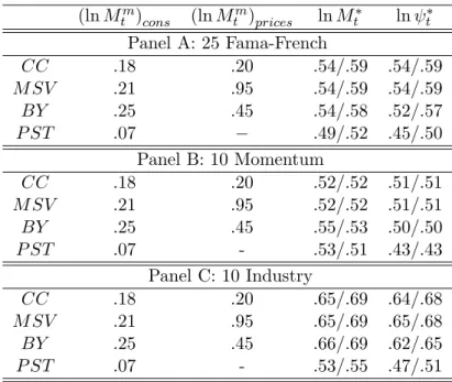
construct entropy bounds for the SDF and its components using quarterly data12 on per capita real personal consumption expenditures on nondurable goods and returns on the 25 Fama-French portfolios over the post war period 1947:1-2009:4 and compare them with theHJ bound.13 We also obtain the non-parametrically extracted (called ”filtered” hereafter) SDF and its components forγ = 10. For the ultimate consumption risk model, we set S= 11 quarters because the fit of the model is the greatest at this value as shown in Parker and Julliard (2005).
Figure 1, Panel A plots the relative entropy (or KLIC) of the filtered and model-implied SDFs and their ψ components as a function of the risk aversion coefficient
γ and the HJ, Q1, M1, and Ψ1 bounds for the contemporaneous consumption risk model in equation (19). The black curve with circles shows the relative entropy of the
12
See Appendix A.4 for a thorough data description.
13
We use the 25 Fama-French portfolios as test assets because they have been used extensively in the literature to test the C-CAPM and also constituted the set of base assets in Parker and Julliard (2005).
model-implied SDF as a function of the risk aversion coefficient. For this model, the missing component of the SDF, ψt, is a constant hence it has zero relative entropy
for all values ofγ, as shown by the grey straight line with triangles. The grey dashed curve and the grey dotted curve show, respectively, the relative entropy as a function of the risk aversion coefficient of the filtered SDF and its missing component. The model satisfies theHJbound for very high values ofγ>64. It satisfies theQ1 bound for even higher values ofγ >72, as shown by the intersection of the horizontal dotted-dashed line and the black curve with circles. The minimum value ofγ at which theM1 bound is satisfied is given by the value corresponding to the intersection of the grey dashed curve and the black curve with circles, i.e. it is the minimum value ofγ for which the relative entropy of the model-implied SDF exceeds that of the filtered SDF. The figure shows that this corresponds toγ = 107. Finally, the Ψ1 bound identifies the minimum value of γ for which the missing component of the model-implied SDF has a higher relative entropy than the missing component of the filtered SDF. Since the former has zero relative entropy while the latter has a strictly positive value for all values of γ, the model fails to satisfy the Ψ1 bound for any value of γ.14
Panel B shows that very similar results are obtained for the Q2, M2, and Ψ2 bounds. The Q2 and M2 bounds are satisfied for values of γ at least as large as 73 and 99, respectively, while the Ψ2 bound is not satisfied for any value ofγ. Overall, as suggested by the theoretical predictions, theQ-bounds are tighter than theHJ-bound, theM-bounds are tighter than the Q-bounds, and the Ψ-bounds are tighter than the
M-bounds.
We also construct confidence bands for the above relative entropy bounds using 1,000 bootstrapped samples. The 95% confidence bands for the Q1 and Q2 bounds extend over the intervals [70.0,109.0] and [69.5,109.0], respectively, and those for the
M1 and M2 bounds cover the intervals [94.5,157.5] and [86.0,150.0], respectively.
14Note that Figure 1 plots the relative entropy of the different components of the SDF as functions
of the CRRA. TheQ,M, and Ψ bounds are expressed directly in terms of the risk aversion coefficient (vertical lines). The Q-bound could have alternatively been expressed in terms of entropy, i.e., as a horizontal line atD(Q∗||P) and D(P||Q∗) in Panels A and B, respectively. One could then have determined what the required minimum CRRA was to satisfy these bounds by computing the minimum CRRA such that the relative entropy of the resulting SDF was at least as large as D(Q∗||P) or D(P||Q∗). However, note that theM and Ψ bounds depend on the CRRA and, therefore, cannot be expressed as horizontal lines. We, therefore, choose to represent all the bounds directly in terms of the CRRA (as vertical lines).
0 20 40 60 80 100 120 0.0 0.2 0.4 0.6 0.8 Panel A γ KL
IC KLIC of model implied:M
t ψt Entropy Bounds: Q M Ψ 0 20 40 60 80 100 120 0.0 0.2 0.4 0.6 0.8 Panel B γ KL
IC KLIC of model implied:M
t ψt Entropy Bounds: Q M Ψ
Figure 1: The figure plots the KLIC of the model SDF,Mt=δ
Ct Ct−1
−γ
, and the modelψ(equal
to zero in this case), as well as theQ,M and Ψ bounds as function of the risk aversion coefficient. TheQ(M) bound is satisfied when the KLIC of Mt is above it, while the Ψ bound is satisfied when the KLIC ofψt is above it. Panels A and B show the results whenψt∗is estimated using the relative entropy minimization procedures in Equations (6) and (4), respectively, using quarterly data over 1947:Q1-2009:Q4 and the 25 Fama-French portfolios as test assets.
Finally, the Ψ1 and Ψ2 bounds are not satisfied for any finite value of the risk aversion coefficient in any of the bootstrapped samples. The bootstrap results reveal two points. First, it demonstrates the robustness of our approach - the two different definitions of relative entropy produce very similar results. Second, the confidence bands are quite tight in contrast with the large values of the standard error typically obtained when using GMM type approaches to estimate the risk aversion parameter.
Figure 2 presents analogous results to Figure 1 for the ultimate consumption risk model in equation (20). PanelA shows that theHJ,Q1, andM1 bounds are satisfied for γ > 22, 23, and 46, respectively. These are almost three times, more than three times, and more than two times smaller, respectively, than the corresponding values in Figure 1, Panel A, for the contemporaneous consumption risk model. As for the latter model, the Ψ1 bound is not satisfied for any value ofγ. PanelB shows that the
Q2 and M2 bounds are satisfied forγ >24 and 47, respectively, while the Ψ2 bound is not satisfied for any value of γ. The bootstrapped 95% confidence bands for the
and those for the M1 andM2 bounds cover the intervals [36.0,60.0] and [40.0,74.0], respectively. Also, similar to the contemporaneous consumption risk model, the Ψ1 and Ψ2 bounds are not satisfied for any finite value of the risk aversion coefficient in any of the bootstrapped samples.
0 20 40 60 80 100 120 0.0 0.2 0.4 0.6 0.8 1.0 Panel A γ KL
IC KLIC of model implied:M
t ψt Entropy Bounds: Q M Ψ 0 20 40 60 80 100 120 0.0 0.2 0.4 0.6 0.8 1.0 Panel B γ KL
IC KLIC of model implied:M
t ψt Entropy Bounds: Q M Ψ
Figure 2: The figure plots the KLIC of the model SDF, Mt = δ1+S
C
t+S Ct−1
−γ
Rft,t+S, and their unobservable components (ψt∗, and the modelψ(equal to zero in this case), as well as theQ,M and Ψ bounds as function of the risk aversion coefficient. TheQ(M) bound is satisfied when the KLIC of Mt is above it, while the Ψ bound is satisfied when the KLIC ofψt is above it. Panels A and B show the results whenψ∗t is estimated using the relative entropy minimization procedures in Equations (6) and (4), respectively, using quarterly data over 1947:Q1-2009:Q4 and the 25 Fama-French portfolios as test assets.
It is important to notice that, even though the best fitting level for the RRA coefficient for the ultimate consumption risk model is smaller than 10 (ˆγ = 1.5), and at this value of the coefficient the model is able to explain about 60% of the cross-sectional variation in returns across the 25 Fama-French portfolios, all the bounds reject the model for low RRA, and the Ψ bounds are not satisfied for any level of RRA. This stresses the power of the proposed approach.
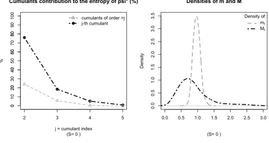
The above results indicate that our entropy bounds are not only theoretically, but also empirically, tighter than the HJ variance bounds. Using the cumulants decomposi-tion introduced in the previous Secdecomposi-tion, we can identify the informadecomposi-tion content added by taking into account higher moments of the SDF and its components. In particular,
0 20 40 60 80 100
Cumulants contribution to the entropy of psi* (%)
(S= 0 ) j = cumulant index % 2 3 4 5 0 10 20 30 40 50 60 70 80 90 cumulants of order >j j-th cumulant 0.0 0.5 1.0 1.5 2.0 2.5 3.0 0.0 0.5 1.0 1.5 2.0 2.5 3.0 3.5 Densities of m and M (S= 0 ) D en si ty Density of: mt Mt
Figure 3: The left panel of the figure plots the relative contribution of the cumulants of ψ∗t to D(P||Ψ∗). The right panel plots the densities of mt :=
Ct Ct−1 −γ and Mt∗ := Ct Ct−1 −γ ψt∗. ψ ∗ t is estimated using the relative entropy minimization procedure in Equation (6), using quarterly data over 1947:Q1-2009:Q4 and the 25 Fama-French portfolios as test assets, for the standard CCAPM with γ= 10.
the statistics in equations (17) (dashed-dotted line) and (18) (dashed line) are plotted in the left panels of Figure 3 (forS = 0) and Figure 4 (for S= 11).
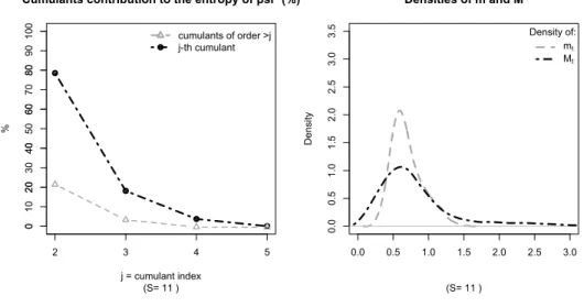
The Figures show that the contribution of the second moment toD(P||Ψ∗) is large – being in the 74-78% range – but that higher moments also play a very important role, with their cumulated contribution being in the 22−26% range. Among these higher moments, the lion’s share goes to the skewness, with it’s individual contribution being about 18% for both S= 0 and S = 11.
The relevance of skewness is also outlined in the right panels of Figure 3 (for
S = 0) and Figure 4 (for S = 11) where the (Epanechnikov kernel estimates of the) densities ofmt:= C t+S Ct−1 −10 Rft,t+S andMt∗:=Ct+S Ct−1 −10
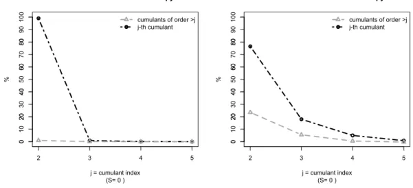
Rt,t+Sf ψ∗t are reported. The figures illustrate that, besides the increase in variance generated by ψ∗, there is also a substantial increase in the skewness of our estimated pricing kernel. This point is also outlined in figures 5 (for S = 0) and 6 (for S = 11) where the left panels report the cumulant decomposition of the entropy ofmt :=
Ct+s Ct−1
−10
Rft,t+S while the right panel reports the cumulant decomposition forMt∗:=mtψt∗. The figures show that the
sources of entropy of our filtered pricing kernel (mtψ∗t) are very different than the ones
0 20 40 60 80 100
Cumulants contribution to the entropy of psi* (%)
(S= 11 ) j = cumulant index % 2 3 4 5 0 10 20 30 40 50 60 70 80 90 cumulants of order >j j-th cumulant 0.0 0.5 1.0 1.5 2.0 2.5 3.0 0.0 0.5 1.0 1.5 2.0 2.5 3.0 3.5 Densities of m and M (S= 11 ) D en si ty Density of: mt Mt
Figure 4: The left panel of the figure plots the relative contribution of the cumulants of ψ∗t to D(P||Ψ
∗
). The right panel plots the densities of mt :=
C t+S Ct−1 −γ Rft,t+S and Mt∗ := C t+S Ct−1 −γ Rft,t+Sψt∗. ψ ∗
t is estimated using the relative entropy minimization procedure in
Equa-tion (6), using qarterly data over 1947:Q1-2009:Q4 and the 25 Fama-French portfolios as test assets,
for the ultimate consumption risk CCAPM of Parker and Julliard (2005) withS= 11 andγ= 10.
mt is generated by its second moment, while higher cumulants have basically no role;
instead, about a quarter (24−25%) of the entropy of mtψ∗t is generated by the third
and higher cumulants.
We now turn to the analysis of the time series properties of the candidate SDFs considered. Figure 7, PanelA plots the time series of the filtered SDF and its compo-nents estimated using equation (6) for γ = 10 for the contemporaneous consumption risk model (S = 0). The dashed line plots the component of the SDF that is a para-metric function of consumption growth,m(θ, t) = (Ct/Ct−1)−γ. The dotted line with
circles plots the filtered unobservable component of the SDF,ψt∗, estimated using equa-tion (6). The black solid line plots the filtered SDF, Mt∗ = (Ct/Ct−1)−γψt∗. The grey
shaded areas represent NBER-dated recessions while the dashed-dotted vertical lines correspond to the major stock market crashes identified in Mishkin and White (2002).15
15
Mishkin and White (2002) identify a stock market crash as a period in which either the Dow Jones Industrial, the S&P500, or the NASDAQ index drops by at least 20 percent in a time window of either one day, five days, one month, three months, or one year. Consequently, in yearly figures, we classy a given year as having a stock market crash if any such event was recorded in that year. Similarly, in quarterly figures, we identify a given quarter as being a crash period if either a crash was registered in that quarter or if the entire year (containing the quarter) was identified by Mishkin and White as a stock market crash year.
0 20 40 60 80 100
Cumulants contribution to the entropy of m
(S= 0 ) j = cumulant index % 2 3 4 5 0 10 20 30 40 50 60 70 80 90 cumulants of order >j j-th cumulant 0 20 40 60 80 100
Cumulants contribution to the entropy of M*
(S= 0 ) j = cumulant index % 2 3 4 5 0 10 20 30 40 50 60 70 80 90 cumulants of order >j j-th cumulant
Figure 5: The left panel of the figure plots the contribution of the cumulants of
Ct Ct−1 −γ to D P|| Ct Ct−1 −γ
. The right panel plots the contribution of the cumulants of Ct
Ct−1 −γ ψt∗ to D P|| Ct Ct−1 −γ ψt∗
. ψt∗is estimated using the relative entropy minimization procedure in Equation (6), using qarterly data over 1947:Q1-2009:Q4 and the 25 Fama-French portfolios as test assets, for
the standard CCAPM withγ= 10.
0 20 40 60 80 100
Cumulants contribution to the entropy of m
(S= 11 ) j = cumulant index % 2 3 4 5 0 10 20 30 40 50 60 70 80 90 cumulants of order >j j-th cumulant 0 20 40 60 80 100
Cumulants contribution to the entropy of M*
(S= 11 ) j = cumulant index % 2 3 4 5 0 10 20 30 40 50 60 70 80 90 cumulants of order >j j-th cumulant
Figure 6: The left panel of the figure plots the contribution of the cumulants ofCt+S Ct−1 −γ Rft,t+S to D P||Ct+S Ct−1 −γ Rft,t+S
. The right panel plots the contribution of the cumulants of
C t+S Ct−1 −γ Rft,t+Sψt∗toD P||Ct+S Ct−1 −γ Rft,t+Sψ∗t
. ψ∗t is estimated using the relative entropy mini-mization procedure in Equation (6), using qarterly data over 1947:Q1-2009:Q4 and the 25 Fama-French portfolios as test assets, for the ultimate consumption risk CCAPM of Parker and Julliard (2005) with S= 11 andγ= 10.
The figure reveals two main points. First, the estimated SDF has a clear business cycle pattern, but also shows significant and sharp reactions to financial market crashes that do not result in economy-wide contractions. Second, the time series of the SDF almost coincides with that of the unobservable component. In fact, the correlation between the two time series is .996. The observable consumption growth component of the SDF, on the other hand, has a correlation of only.06 with the SDF. Therefore, most of the variation in the SDF comes from variation in the unobservable component,ψ, and not from the consumption growth component. In fact, the volatility of the SDF and its unobservable component are very similar with the latter explaining about 99% of the volatility of the former, while the volatility of the consumption growth component accounts for only about 1% of the volatility of the filtered SDF. Similar results are obtained in PanelB that plots the time series of the filtered SDF and its components estimated using equation (4) for γ= 10.
Finally, Figure 8, Panel A plots the time series of the filtered SDF and its compo-nents estimated using equation (6) forγ = 10 for the ultimate consumption risk model (S = 11). The figure shows that, as in the contemporaneous consumption risk model, the estimated SDF has a clear business cycle pattern, but also shows significant and sharp reactions to financial market crashes that do not result in economy wide contrac-tions. However, differently from the latter model, the time series of the consumption growth component is much more volatile and more highly correlated with the SDF. The volatility of the consumption growth component is 21.7%, more than 2.5 times higher than that for the standard model. The correlation between the filtered SDF and its consumption growth component is .37, an order of magnitude bigger than the correlation of .06 in the contemporaneous consumption risk model. This explains the ability of the model to account for a much larger fraction of the variation in expected returns across the 25 Fama-French portfolios for low levels of the risk aversion coeffi-cient. In fact, the cross-sectional R2 of the model is 54.1% (for γ = 10), an order of magnitude higher than the value of 5.2% for the standard model. However, the corre-lation between the ultimate consumption risk SDF and its unobservable component is still very high at.92, showing that the model is missing important elements that would further improve its ability to explain the cross-section of returns. Similar results are
obtained in PanelB that plots the time series of the filtered SDF and its components estimated using equation (4) for γ= 10.
Overall, the results show that our methodology provides useful diagnostics for dy-namic asset pricing models. Moreover, the very similar results obtained using the two different types of relative entropy minimization in equations (4) and (6) suggest robustness of our approach.
IV
Application to More General Models of Dynamic Economies
Our methodology provides useful diagnostics to assess the empirical plausibility of a large class of consumption-based asset pricing models where the SDF, Mt, can be
factorized into an observable component consisting of a parametric function of con-sumption,Ct, as in the standard time-separable power utility model, and a potentially
unobservable one, ψt, that is model-specific. In this Section, we apply it to a set
of ”winners” asset pricing models, i.e. frameworks that can successfully explain the Equity Premium and the Risk Free Rate Puzzles with “reasonable” calibrations. In particular, we consider the external habit formation models of Campbell and Cochrane (1999) and Menzly, Santos, and Veronesi (2004), the long-run risks model of Bansal and Yaron (2004), and the housing model of Piazzesi, Schneider, and Tuzel (2007). We apply our methodology to assess the empirical plausibility of these models in two ways. First, since our methodology delivers an estimate of the time-series of the SDF, for each model considered we compare the estimated time-series with the model-implied one. Second, for each model we compute the values of the power coefficient,γ, at which the model-implied SDF satisfies theHJ,Q,M, and Ψ bounds.
In the next sub-section we present the models considered. The reader familiar with these models can go directly to Section IV.2, that reports the empirical results, without loss of continuity. A detailed data description is presented in Appendix A.4.
IV.1 The Models Considered
IV.1.1 External Habit Formation Model: Campbell and Cochrane (1999)
In this model, identical agents maximize power utility defined over the difference be-tween consumption and a slow-moving habit or time-varying subsistence level. The
SDF is given by Mtm= (Ct/Ct−1)−γ | {z } m(θ,t) δ(St/St−1)−γ | {z } ψm t , (21)
whereδ is the subjective time discount factor,γ is the curvature parameter that pro-vides a lower bound on the time varying coefficient of relative risk aversion,St= CtC−Xt t
denotes the surplus consumption ratio, andXtis the habit component. Note that the
ψm component depends on the surplus consumption ratio, S, that is not directly ob-served. To obtain the time series ofψm, we extract the surplus consumption ratio from observed data using two different procedures.
First, we extract the time series of the surplus consumption ratio from consumption data. In this model, the aggregate consumption growth is assumed to follow an i.i.d.
process:
∆ct=g+υt, υt∼i.i.d.N 0, σ2
.
The log surplus consumption ratio evolves as a heteroskedasticAR(1) process:
st= (1−φ)s+φst−1+λ(st−1)υt, (22)
wherest:= lnSt and sis the steady state log surplus consumption ratio and
λ(st) = 1 S p 1−2 (st−s)−1, ifst≤smax 0, ifst> smax , smax=s+ 1 2 1−S2 , S =σ r γ 1−φ.
For each value ofγ, we use the calibrated values of the model preference parameters (δ,φ) in Campbell and Cochrane (1999), the sample mean (g) and volatility (σ) of the consumption growth process, and the innovations in real consumption growth, υbt =
∆ct−g, to extract the time series of the surplus consumption ratio using equation (22)
and, thereby, obtain the time series of the model-implied SDF and itsψm component. Second, in this model, the equilibrium market-wide price-dividend ratio is a func-tion of the surplus consumpfunc-tion ratio alone, although the form of the funcfunc-tion is not available in closed-form. Using numerical methods, we invert this function to extract
the time series of the surplus consumption ratio from the historical time series of the price-dividend ratio and, thereby, obtain the time series of the model-implied SDF and its ψm component from equation (21).
IV.1.2 External Habit Formation Model: Menzly, Santos, and Veronesi (2004)
In this model, the SDF is analogous to the Campbell and Cochrane (1999) one disussed above. The aggregate consumption growth is also assumed to follow ani.i.d. process:
dct=µcdt+σcdBt,
where µc is the mean consumption growth, σc > 0 is a scalar, and Bt is a Brownian
motion. The point of departure from the Campbell and Cochrane (1999) framework is that Menzly, Santos, and Veronesi (2004) assume that theinverse surplus consumption ratio,Yt:= S1t, follows a mean reverting process that is perfectly negatively correlated
with innovations in consumption growth:
dYt=k Y −Yt
dt−α(Yt−λ) [dct−E(dct)] , (23)
whereY is the long run mean of the inverse surplus consumption ratio andkcontrols the speed of mean reversion. To obtain the time series of ψm (the model implied ψ
component), we extract the surplus consumption ratio from observed data using two different procedures.
First, for each value of γ,16 we use the calibrated values of the model parameters
δ,k,Y,α,λ
in Menzly, Santos, and Veronesi (2004), the sample values of µc and
σc, and the innovations in real consumption growth, dBdt =
[dct−E(dct)]
σc , to extract the
time series of the surplus consumption ratio, and that allows us to compute the time series of the model-implied SDF.
Second, in this model, the equilibrium price-consumption ratio of the total wealth portfolio is a function of the surplus consumption ratio alone. However, this function
16Note that the Menzly, Santos, and Veronesi (2004) model assumes that the representative agent has
log utility, i.e. γis set equal to 1, in order to derive the closed-form solution for the price-consumption ratio. For other values ofγ, the model does not admit a closed-form solution. Nevertheless, the pricing kernel is well defined even if γ is different than one, hence we will be considering this more general case.
is not available in closed-form except for γ = 1. Therefore, we rely on log-linear approximations to the return on the total wealth portfolio to express the equilibrium log price-consumption ratio as an affine function of the log surplus consumption ratio for all values ofγ. Details of this procedure are described in Appendix A.5. We, then, invert this affine function to extract the time series of the surplus consumption ratio from the historical time series of the market-wide price-dividend ratio and, thereby, obtain the time series of the model-implied SDF and its ψm component from equation (21). Note that approximating the total wealth price-consumption ratio by the market-wide price-dividend ratio is the approach used by Menzly, Santos, and Veronesi (2004).
IV.1.3 Long-Run Risks Model: Bansal and Yaron (2004)
The Bansal and Yaron (2004) long-run risks model assumes that the representative consumer has the version of Kreps and Porteus (1978) preferences adopted by Epstein and Zin (1989) and Weil (1989) for which the SDF is given by
Mt+1m =δθ Ct+1 Ct −θρ Rθ−1c,t+1,
whereRc,t+1 is the unobservable gross return on an asset that delivers aggregate
con-sumption as its dividend each period,δ is the subjective time discount factor, ρis the elasticity of intertemporal substitution, θ:= 1−1/ρ1−γ , and γ is the relative risk aversion coefficient.
The aggregate consumption and dividend growth rates, ∆ct+1 and ∆dt+1,
respec-tively, are modeled as containing a small persistent expected growth rate component,
xt, that follows an AR(1) process with stochastic volatility, and fluctuating variance,
σt2, that evolves according to a homoscedastic linear mean reverting process.
Appendix A.6 shows that, for the log-linearized model, the log of the SDF and its
ψm component are given by
lnMt+1m = c2∆ct+1 | {z } lnm(θ,t+1) +c1+c3xt+1+c4σt+12 +c5xt+c6σt2 | {z } lnψm t+1 (24)
where the parameters (c1, c2, c3, c4, c5, c6) are known functions of the underlying time