Cost-Sensitive Decision Trees with Completion Time Requirements

KRANNERT SCHOOL OF

MANAGEMENT

Purdue University

West Lafayette, Indiana

Cost-Sensitive Decision Trees with Completion Time

Requirements

By

Hung-Pin Kao

Kwei Tang

Jen Tang

Paper No. 1264

Date: September, 2010

Institute for Research in the

Behavioral, Economic, and

Management Sciences

Abstract—In many classification tasks, managing costs and

completion times are the main concerns. In this paper, we assume that the completion time for classifying an instance is determined by its class label, and that a late penalty cost is incurred if the deadline is not met. This time requirement enriches the classification problem but posts a challenge to developing a solution algorithm. We propose an innovative approach for the decision tree induction, which produces multiple candidate trees by allowing more than one splitting attribute at each node. The user can specify the maximum number of candidate trees to control the computational efforts required to produce the final solution. In the tree-induction process, an allocation scheme is used to dynamically distribute the given number of candidate trees to splitting attributes according to their estimated contributions to cost reduction. The algorithm finds the final tree by backtracking. An extensive experiment shows that the algorithm outperforms the top-down heuristic and can effectively obtain the optimal or near-optimal decision trees without an excessive computation time.

Index Terms—classification, decision tree, cost and time

sensitive learning, late penalty

I. INTRODUCTION

ecision trees are an attractive method for classification tasks, because they can efficiently generate rules easy to interpret and understand [1]. Many decision-tree induction algorithms have been developed for a wide range of applications, including medical diagnosis, fraud detection, credit scoring, and direct marketing. The majority of existing algorithms, such as ID3, CART, and C4.5, are greedy heuristics for maximizing classification accuracy, which work in a top-down manner using a statistic measure or information gain as the criterion in selecting an attribute to produce further splits [2].

In many classification applications, managing costs and completion times are main concerns. For example, in designing a medical diagnosis procedure, the costs of Hung-pin Kao is with the Krannert School of Management, Purdue University, West Lafayette, Indiana 47907, U.S.A. E-mail: [email protected], Tel: 765-496-2240. Fax: 765-494-4360.

Kwei Tang is with the Krannert School of Management, Purdue University, West Lafayette, Indiana 47907, U.S.A. E-mail:

[email protected], Tel: 765-494-4464. Fax: 765-494-4360.

Jen Tang is with the Krannert Graduate School of Management, Purdue University, West Lafayette, IN 47907, U.S.A. E-mail: [email protected], Tel: 765-494-4497, Fax: 765-494-4360.

performing tests and the economic consequences incurred by erroneous results could be dominating factors. Furthermore, the completion time of a diagnosis procedure is critical for some illnesses like heart attack and stroke, because the fatality rate and chance of permanent disability increase dramatically if treatment is delayed. Similar scenarios are found in fraud detection, customer retention, and other applications.

The cost-sensitive (CS) decision tree is the research area that explicitly considers cost minimization as the goal in developing tree-induction algorithms. Two costs are commonly considered: the cost of using attributes (attribute cost) and the costs incurred by misclassification. Turney [3] applied the genetic algorithm to search for a decision tree with the lowest misclassification cost. Ling et al. [4] developed a top-down heuristic for minimizing the sum of the attribute and misclassification costs. Ling et al. [5] further proposed a lazy-learning heuristic, which allows discounts in attribute costs when several attributes can be evaluated together. For additional references for the CS trees, please refer to Ling et al. [5].

To our best knowledge, Arnt and Zilberstein [6] and Chen et al. [7] are the only studies that explicitly consider both costs and completion times in classification tasks. Arnt and Zilberstein assumed an increasing cost function of the completion time in addition to attribute and misclassification costs. They used the Markov decision process to solve a cost-minimization problem. Chen et al. [7] required all classifications be finished before a common deadline. Their top-down heuristic uses the cost-reduction rate (the cost reduction per unit time) as the criterion for selecting splitting attributes. After the tree has been developed, a local search is performed to utilize slack times in the tree for possible improvements.

We generalize the problem proposed by Chen et al. [7] by assuming that the required completion times are determined by class labels. This completion time requirement is applicable to many classification tasks. For example, there are several types of heart disease with different severity levels, including coronary artery disease, heart attack, heart failure, arrhythmia, etc. A heart attack is much more serious than coronary artery disease and requires immediate medical attention. Therefore, a shorter completion time should be set for the diagnosis of a patient with a heart attack than one with coronary artery disease. Similarly, in customer retention, customers may be categorized according to their times to churn. Customers who will soon switch to another service

Cost-Sensitive Decision Trees

with Completion Time Requirements

Hung-Pin KAO, Kwei TANG, and Jen TANG

need to be identified more quickly than those who may stay for a longer period of time. Similarly, in fraud detection, the priority should be to identify more serious fraudulent cases in a shorter time. To incorporate this requirement, we add late penalties to the total cost considered in the tree induction. This type of completion time requirement enriches the classification problem, but, at the same time, poses a challenge to developing algorithms for tree induction. For convenience, we name the proposed research problem as the cost-sensitive-with-late-penalty (CSLP) decision tree.

It is well known that the traditional top-down approach is computationally efficient. However, it has significant drawbacks. In particular, the criteria used in selecting splitting attributes are “myopic” in nature, reflecting only instant benefits at “current” tree nodes. As a result, the attributes selected in early stages may have little value in the final tree. Similarly, the tree growth may be stopped prematurely, because the same criteria are used. For the problem under consideration, an additional issue is the difficulty in adequately assessing an attribute’s contribution to the late penalty cost in early stages of the tree induction, because late penalties may occur only at later stages. These issues motivate the development of an innovative algorithm in this paper.

Essentially, our proposed algorithm produces multiple tree candidates by allowing more than one splitting attribute at each node in the tree-induction process. The user can specify the maximum number of candidate trees to control the required computational efforts. In the induction process, an allocation scheme is used to dynamically distribute the given number of candidate trees to splitting attributes according to their estimated contributions to cost reduction. The algorithm finds the grown tree with the minimum cost as the solution by backtracking. Overall, it works like an exploration aiming to locate the optimal solution in a limited but promising area in the solution space. In contrast, the traditional top-down approach forces a selection of one splitting attribute at a given node and develops only one decision tree in the induction process. For convenience, we use EXP as the name of our proposed algorithm.

This paper is organized as follows. In section II, we define the problem, and in section III, we present the proposed tree induction algorithm with two illustrative examples. In section IV, we perform an extensive experiment to evaluate the performance of the algorithm. In section V, we summarize the results and discuss possible extensions.

II.PROBLEM DEFINITION

Consider a training dataset consisting of N records with K attributes, X1, X2, …, XK, and a class label (target variable), Y.

Let y1, y2, …, and yM be the levels of Y. The attributes are used

to develop a decision tree by a sequence of splits, and each leaf of the tree is assigned a predicted label value for all the instances at the leaf. For simplicity, we assume that all the attributes are categorical and all the records do not contain missing values.

Let Tj and Cj denote the time and cost, respectively, for measuring attribute Xj, and Vk the deadline for classifying an instance in class k. If it takes a time longer than Vk to classify an instance in class k, a late penalty Pk is incurred. If a class j instance is classified into class k, a misclassification cost of CM(j, k) is incurred, where CM(j, k) = 0 if j = k.

For a given decision tree R with Q leaf nodes, we define the follow notation: Leaf(R) as the set of leafs {l1, l2, …, lQ}; ψ(li)

the set of attributes used in the path from the root node to leaf li; N(li) the number of instances at leaf li; N(yk, li) the number of class k (Y = yk) instances at li.

Three costs are considered in developing a decision tree: the misclassification cost (CM), attribute cost (CA), and late cost (CL). We derive these costs for a given tree as follows. At leaf li, in order to minimize the total misclassification cost associated with the N(li) instances, the class label assigned to the leaf, ˆ, i l Y is determined by:

∑

= ∈ × = M j i j M M k l C jk N y l Y i 1 } ,..., 1 { ( , ) ( , ). min arg ˆ (1)

Consequently, the total misclassification cost for the instances at li is

∑

= × = M j i j l M i M l C jY N y l C i 1 ). , ( ) ˆ , ( ) ( (2)

And the total misclassification cost associated with the tree

R is .) ( ) ( ) (

∑

∈ = R Leaf l i M M i l C R TC (3)

The total attribute cost for the instances at li is determined by ), ( ) ( ) (l i X j i A l C N l C i j × =

∑

∈ψ (4) and the total attribute cost for the tree is

.) ( ) ( ) (

∑

∈ = R Leaf l A A R C l TC (5)

The time for an instance to reach leaf li is given by . ) ( ) (

∑

∈ = i j l X j i T l t ψ (6) For an instance at li with Y = yk, the late penalty is Pj if t(li) >

Vk; and 0, otherwise. We define an indicator variable:

⎩ ⎨ ⎧ > ≤ = , ) ( if , 1 ) ( if , 0 ) , ( k i k i i V l t V l t k l I (7)

using which, the total late penalty at li is given as , ) , ( ) ( 1

∑

= × = M k i j i P l P I l k C (8)

and the total late penalty for the tree is

.) ( ) ( ) (

∑

∈ = R Leaf l i P P i l C R TC (9)

Combining the three cost components, the total costs for leaf li and tree R are given, respectively, as

) ( ) ( ) ( ) (l_i C_M l_i C_A l_i C_P l_i C = + + (10) and .) ( ) ( ) (

∑

∈ = R Leaf l i i l C R TC (11)

The optimal tree is the one with the minimum TC(R). In the next section, we discuss the tree-induction algorithm with the objective to find the optimal tree.

III. TREE-INDUCTION ALGORITHM

A.The EXP algorithm

We present the proposed algorithm for the CSLP decision tree induction. We first discuss the structure of the algorithm and then the allocation scheme of trees to the solution space. Two examples are used to illustrate the algorithm.

Let qmax be the maximum number of candidate trees allowed in the induction process. The algorithm starts with the root node by using the EXP function in Figure 1 to allocate qmax to the K attributes. This process is applied recursively at each new node added to the tree. When no splitting attributes are available, no sub-trees will be produced, and when the available number of trees is 1 or smaller, a top-down myopic heuristic is used to construct the sub-tree from the node. Once all sub-trees are fully grown from a node, the sub-tree with the smallest cost is selected as the “optimal” sub-tree rooted at the node.

Let q denote the number of trees available for allocation at node n (q = qmax at the root node). The magnitude of q determines the depth of the search at node n: a larger q implies a more extensive search. Therefore, if the user gives a larger qmax, the decision tree produced by the EXP algorithm is likely to have a lower cost. However, it also requires more computation time. When qmax is sufficiently large, the algorithm is equivalent to an exhaustive search, and when qmax is 1, it is basically a simple top-down heuristic.

================== Insert Fig. 1 here ================== Fig. 1. The EXP algorithm.

From the above description, it is evident that the key element of the algorithm is the scheme for allocating the available number of candidate trees at each new node in the tree-induction process. We first derive the estimated instant benefit (EIB) of a splitting attribute at a given node to be used in the allocation scheme.

Let b(n, Xi) denote the net cost reduction resulting from splitting n on Xi. We use children(n, Xi) to denote the set of child nodes created from splitting n by Xi, and obtain:

.) ( ) ( ) , ( ) , (

∑

∈ − = i X n children l i C n C l X n b (12)

After the split using Xi, the classification time of all instances

in n is t(n) + Ti. At this point, late penalties may not have been

realized for some instances, depending on their labels. Assume Vk > t(n) + Ti. For the instances of class k at node n, it is difficult to determine whether or how much the late penalty will eventually be realized if the tree growth continues. Note that, in the grown tree, the total late penalty for these instances must be between 0 and N(y_k,n)×P_k. We pro-rate the penalty

cost according to the ratio of the attribute time, Ti, to the deadline, Vk, in estimating the late penalty resulting from splitting n on Xi. Let A(n, Xi) denote the estimated late penalty by attribute Xi determined by:

∑

+ > ∈ × × = } ) ( | { ) / ( ) , ( ) , ( Ti n t V y y k i k k i j j k V T P n y N X n A . (13)

Consequently, the EIB of using Xi as the splitting attribute at n, denoted by B(n, Xi), is given by:

) , ( ) , ( ) , (n X_i b n X_i An X_i B = − . (14)

If all available splitting attributes have the same EIBs, we will distribute q evenly among them. Otherwise, an attribute is considered more preferable if it has a larger EIB and, thus, is given a larger share of q. However, no available splitting attributes should be excluded, even those with negative EIBs, because of the possibility that using them may still lead to a good result.

Let Bmin and Bmax be, respectively, the smallest and largest EIBs of the splitting attributes available at the node under consideration. We define for each available attribute:

)], , max( [ ) , (n X Bmin p z Bmax B d_i = _i − − × (15)

where p > 0 and z > 0 are selected by the user. We propose the following allocation scheme for assigning the number of trees to an available attribute Xi:

. / ) ,..., 1 (

∑

∈ × = K j j i i q d d q (16)

Note that [Bmin – p × max(z, Bmax)] represents the reference value for measuring each attribute’s potential of yielding a low-cost sub-tree by splitting on Xi, and z ensures that all di’s are positive. The user can adjust p to control the sensitivity of the allocation to the dispersion in B(n, Xi). When a small p is used, the values of di’s tend to have a smaller variation, leading to smaller differences in the allocation. Note that it is possible, under the scheme, to allocate an excessive number to a splitting attribute. We may ignore the unused number of trees or distribute it to other attributes.

When q is equal to or less than 1, we use a top-down heuristic to produce a sub-tree from n using B(n, Xi) as the criterion in selecting splitting attributes. It is expected that the selection of the splitting criterion does not affect EXP’s performance as significantly as the allocation scheme does. The first reason is that the heuristic algorithm usually is used near the leaves of a decision tree, where the choices are usually correct. Second, if the allocation scheme properly places large numbers of trees on important splitting attributes, finding optimal or near optimal trees are less dependent on the heuristic method.

B.Examples

We use two examples to illustrate the proposed algorithm and compare it with the brute-force search algorithm, abbreviated by OPT(imum). The dataset, “Heart Cleveland” (HRT296), is used in the first example, which contains the heart disease diagnosis data from 296 patients.1 _{The class}

1 _{The original dataset at UCI data mining repository has 303 records. We} removed 5 records because of missing values.

label indicates the presence or absence of a heart disease, and 13 attributes include patients’ demographics and medical test results. This dataset has been widely used for classification benchmarking in machine learning. The “Hepatitis Domain” dataset (HPT151) is used in the second example. It contains diagnosis data of 151 hepatitis patients with two classes, survivors and victims, and 19 attributes.2 _{The two datasets are}

available at the UC Irvine Machine Learning Repository. All numeric attributes are discretized, using the method by Fayyad Irani [8]. The cutoff points are selected to maximize the information gain and are tested against the MDLP criterion.

The cost and time parameters for the both datasets are given in the Appendix under Setting HRT296-C and Setting HPT151-C, respectively. Note that these parameters are randomly generated, because the original datasets do not contain the late penalty information. We will explain the methods of generation in the next section, where we conduct an extensive numerical evaluation of the algorithm.

The EXP algorithm with qmax = 200 and the brute-force algorithm yield the optimal decision tree given in Part (a) of Figure 2. We include the numbers of instances associated with the classes and time information along the tree induction. We observe that many attributes with short attribute times are used, such as cp, sex, and age. Approximately 17.6% of the instances shown in the dashed rectangle in the figure have passed their respective deadlines, incurring an average late penalty cost of $33.11 per instance. The overall misclassification rate is 22.6%, and the average cost of misclassification is $260.14. The average attribute cost is $9.81, and the average total cost per instance is $303.05. When qmax is set to 200, the EXP algorithm took 390 milliseconds to complete the induction.3 _{In comparison, it}

requires 975 seconds for the brute-force search to find the optimal decision tree.

For this example, the EXP algorithm finds the optimal tree, when qmax is set at or above 200. As discussed, if qmax = 1, the EXP algorithm is equivalent to a top-down heuristic based on the estimated instant benefit as the attribute selection criterion. Part (b) of Figure 2 shows the tree obtained by such an approach. The tree is relatively smaller and has an average cost of $339.45 (higher than the optimum by 12.0%). A noticeable difference is observed at node #3, where the top-down heuristic stops splitting because of a negative EIB. In contrast, the EXP algorithm continues exploring the possibility of reducing the cost although the cost increases temporarily from $39,141 to $40,762.5 (the sum of $3,140 at node #6, $29,650 at node #7, and $7,962.5 at node #8). As shown in the optimal tree, the gains in classification accuracy in the leaves under node #3 eventually justify the splits at node #3.

==================

2 _{The original dataset consists of 155 records. Four records are removed} because of missing values.

3 _{We implemented the algorithms in Java on a PC with CPU Intel® Core™} 2 Duo E6750 under Windows® Vista and JDK 1.6.0.

Insert Fig. 2 here ==================

Fig. 2. The decision trees generated by the EXP algorithm with HRT296 dataset (test case HRT296_C).

================== Insert Fig. 3 here ================== Fig. 3. The effect of qmax.

When a large number of attributes is encountered, a much larger qmax is required for the EXP algorithm to find the optimal tree. We use the second dataset, HPT151, with a relatively large number of attributes to show the effects of qmax. Part (a) of Figure 3 reports the average costs per instance as we increase qmax from 100 to 12,000. For comparison, we also plot a horizontal line near the top of the figure to indicate the average cost achieved by the top-down heuristic (i.e., qmax = 1). The total cost appears as a step function of qmax and becomes steady after 10,000 since the optimal tree has been found. Note that the total cost of the top-down approach is 84% higher than that of the optimal tree, and that the difference is reduced to 28.8% for qmax = 200, and 8.1% for qmax = 4,000.

Part (b) shows the run time as a function of qmax. The algorithm ends at less than 15 milliseconds when qmax = 1. As expected, the time increases when a large qmax is used. When

qmax = 4,000, the algorithm yields a solution within 8.1% from

the optimal tree in 10.1 seconds. When qmax = 10,000, the EXP algorithm obtains the optimal decision tree in 17.0 seconds. The overall results suggest that, with a moderate qmax, the algorithm can find a near optimal solution within a reasonable time. In contrast, it requires 824.8 seconds for the brute-force search to find the optimal solution.

The allocation scheme for distributing the number of candidate trees should affect the performance of the EXP algorithm. It is expected that a smaller qmax is required for obtaining the optimal solution, if a more efficient allocation scheme is used. To evaluate the performance of the proposed allocation scheme, we compared it with an equal allocation scheme, which distributes the number of candidate trees evenly to all available splitting attributes. Figure 4 shows the average per-instance costs of the two schemes as functions of qmax. In the entire range, the even allocation performs better only when qmax = 200. The equal allocation scheme yields the optimal tree when qmax is at least 26,000, whereas only 10,000 is required for the proposed allocation scheme based on EIB.

The equal allocation method is similar to building a tree by choosing a splitting attribute randomly. We find when qmax is very small, e.g., 100, the EXP algorithm based on the equal allocation method still significantly outperforms the top-down heuristic, confirming the effectiveness of the proposed strategy of allowing multiple candidate decision trees in the tree- induction process.

IV. EXPERIMENT

The results reported in the two examples suggest that the EXP algorithm is effective in finding the optimal tree. In this section, we perform an extensive experiment to evaluate the algorithm by comparing it with the brute-force search, and the top-down heuristic using EIB for selecting splitting attributes. Four datasets from the UC Irvine Machine Learning Repository with multiple cost and time settings are used in the experiment.4 _{The setups of the experiment are discussed in the}

next subsection.

A.Setups

The first two datasets, HRT296 and HPT151, have been discussed in the last section. The third, BRT277, contains data of breast cancer diagnoses, and the fourth, DBT768, diabetes diagnoses. We have pre-processed the datasets by removing missing values and discretizing numeric attributes. Table I contains a brief description of the datasets after pre-processing.

TABLEI

THE DATASETS USED FOR PERFORMANCE TESTS

================== Insert TABLE I here ==================

We use the following three attribute cost and time settings: A.The values are available in the literature.5

B.The attribute costs and times for demographic attributes are set at $1 and 1 unit, respectively. Remaining costs and times are randomly generated, respectively, from the uniform distributions with ranges of [$5, $50] and [10 units, 100 units].

C.The attribute cost and time for demographic attributes are set at $1 and 1 unit, respectively. Remaining costs and times are randomly generated, respectively, from the uniform distributions with ranges of [$5, $15] and [10 units, 100 units].

We refer to a test case as (dataset name)_(cost and time setting). For example, HRT296_B represents dataset HRT296 under setting B. Since setting A is not available for the third and fourth datasets, we have 10 test cases in total.

All the test cases, except HPT151_A, share the same misclassification costs ($1,000 and $3,000) and late penalties ($100 and $300). Since the attribute costs for HPT151 used in a previous study are exceptionally low, we change them to $100 for negative instances and $300 for positive instances. The late penalties are $10 and $30, respectively, for less and more severe classes. To synthesize classification deadlines, we first use the brute-force algorithm to find the optimal CS trees and use 70% and 80% of its average completion time as the deadlines of the less and more severe classes, respectively.

4 _{The datasets can be accessed at http://archive.ics.uci.edu/ml/datasets/ .} 5 _{Previous test costs for BRT277 and DBT768 are unavailable. Therefore} we conducted experiments based only on settings B and C for these two datasets.

The cost and time settings are given in the Appendix.

We use qmax = 20,000 for the test cases based on HPT151, and use 1,000 in other cases, unless stated otherwise, and z = 10 and p = 1 for the tree-allocation scheme. The solutions provided by the brute-force search (OPT) are used to evaluate the EXP algorithm in its cost performance. The comparison between the EXP algorithm and the top-down heuristic (TDH) can show the benefits of producing multiple candidate trees in the induction process. Note that using a brute-force search may not be practical when the number of attributes is large. In this experiment, the running time ranges from a few seconds (HRT296) to more than one hour (HPT151).

B.Results

We use bootstrapping in our performance evaluations. For each test case, 50 bootstrap replicates (with the same sample size as the original) were generated from each of the original datasets by simple random sampling with replacement. The EXP algorithm, brute-force search, and a top-down heuristic are applied on each replicate and the average costs per instance are computed for comparisons.

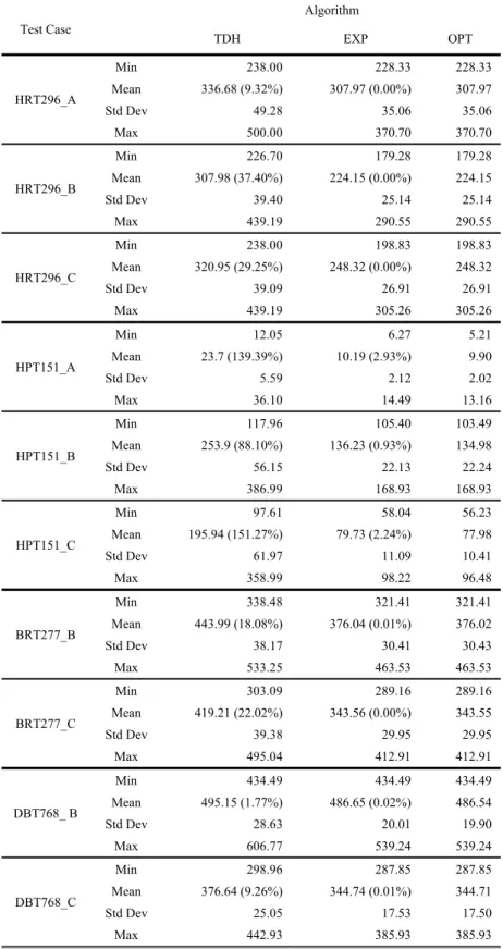
The results are presented graphically by the box-plots in Table II, and summary statistics are reported in Table III. In general, the EXP and the brute-force search produce very similar results, and their average costs are significantly lower than those obtained by the top-down heuristic. For the datasets with a smaller number of attributes, including HRT296, BRT277, and DBT768, the solutions of the EXP algorithm are within 0.02% of the optimal solutions given by the brute-force algorithm. For HPT151, which has a large number of attributes, the difference increases to 2.93% in setting A, 0.93% in setting B, and 2.24% in setting C. The EXP algorithm did not obtain the optimal solution because the given qmax is not large enough; thus, it has to rely on the top-down approach to complete many lower parts of a decision tree. However, the differences are small, especially considering that the computation times of the EXP algorithm are much lower than those of the brute-force search. For example, the brute-force search requires 764 seconds on average to generate the optimal trees for test case HPT151_A, whereas the EXP algorithm takes only 26 seconds.

The results also indicate that the top-down heuristic does not perform well in almost all the test cases. Although its computational time is very short, the average per-instance cost could be significantly higher than that of the optimal solution. Using dataset HPT151 as an example, it takes less than 15 milliseconds to generate a solution. However, its average costs in the three settings are 139.4%, 88.1%, and 151.3% higher than those of the optimal trees.

TABLEII

THE DATASETS USED FOR PERFORMANCE TESTS

================== Insert TABLE II here ==================

SUMMARY STATISTICS FOR COMPARING THE THREE ALGORITHMS. ==================

Insert TABLE III here ==================

In summary, the experiment results support that the EXP algorithm is capable of obtaining optimal or near optimal CSLP trees in very reasonable times. We believe the concept of producing multiple candidate trees in the induction process is promising and can also be used to improve many existing tree algorithms.

V.CONCLUSION

In this paper, we generalize the cost and time-sensitive decision-tree problem proposed by Chen et al. [7] by assuming that required completion times are determined by class labels. This new problem has many potential application fields, including medical diagnosis, customer retention, and fraud detection. Our proposed algorithm for the problem produces multiple candidate trees in the induction process. The user can specify the maximum number of candidate trees to control the required computational efforts. In the induction process, an allocation scheme dynamically distributes the given number of candidate trees to splitting attributes according to their estimated contributions to cost reduction. The algorithm finds the tree with the minimum cost as the final solution by backtracking. An extensive experiment is used to compare the proposed algorithm, brute-force search, and a top-down heuristic. The results show that the algorithm significantly outperforms the top-down heuristic and can effectively obtain the optimal or near-optimal decision trees without an excessive computation time.

There are two possible extensions of this paper to further improve the EXP algorithm. The first is the development of an adaptive allocation scheme to distribute candidate treesin the tree induction process. For example, if EBIs have a very large variation among available splitting variables at a node, the allocation should be more even when q is large. However, when q is small, we may need to focus on few splits with better estimated instant benefits. An allocation scheme based on this concept may improve the performance of the EXP algorithm.

The second possible extension is on the searching strategy of the algorithm. The current search strategy is a deterministic process without considering the results found in the induction process. If we find a tree with a very low cost during the induction process, for example, it may be reasonable to invest more computation resources (i.e., allocate more trees) to its neighboring areas. Therefore, we may use a two-step process to obtain candidate trees. In the first step, we find a number of grown trees based on the EXP algorithm. In the second step, local search is applied to their neighboring areas according to their cost performances. We expect that this two-step process is especially effective when qmax is small.

Finally, we may consider a different problem formulation. In this paper, late penalty is used to incorporate the time

constraints in the model. We may consider the time constraints directly and hope to control the percentages of instances that pass the deadlines. Making this change in model formulation is straightforward. However, developing algorithms to solve the problem could be challenging.

APPENDIX

COST SETTINGS FOR HRT296

Setting A Setting B Setting C

Cost Cost Time Cost Time Cost

Attributes age 1 1 1 1 1 1 sex 1 1 1 1 1 1 cp 1 1 1 1 1 1 trestbps 1 1 11 87 13 38 chol 7.27 240 40.5 52 9.5 15 fbs 5.2 240 12.5 55 13.5 78 restecg 15.5 30 7 38 13.5 98 thalach 102.9 60 26 98 7 55 exang 87.3 60 11.5 73 11 94 oldpeak 87.3 60 24 50 13.5 52 slope 87.3 60 34.5 52 8 58 ca 100.9 60 32.5 21 8.5 96 thal 102.9 60 5 12 11.5 39 Classes Negative Mis. 1000 1000 1000 Late 100 44 100 104 100 96 Positive Mis. 3000 3000 3000 Late 300 50 300 119 300 110

COST SETTINGS FOR HPT151

Setting A Setting B Setting C

Cost Cost Time Cost Time Cost

Attributes SEX 1 1 1 1 1 1 STEROID 1 1 10 70 11.5 38 ANTIVIRALS 1 1 42.5 77 10 15 FATIGUE 1 1 18 12 9 86 MALAISE 1 1 46.5 29 5.5 38 ANOREXIA 1 1 47 66 13 25 'LIVER BIG' 1 1 35 91 5 35 'LIVER FIRM' 1 1 7 20 9.5 77 'SPLEEN PALPABLE' 1 1 35.5 30 8 50 SPIDERS 1 1 41.5 75 12.5 94 ASCITES 1 1 36 15 8 78 VARICES 1 1 8.5 38 9 76 BILIRUBIN 7.27 19 31 97 13.5 18 SGOT 7.27 21 24.5 90 12.5 56 ALBUMIN 7.27 23 18 87 14 16 HISTOLOGY 1 1 15 10 14.5 35 Classes Negative Mis. 100 1000 1000 Late 10 18 100 163 100 225 Positive Mis. 300 3000 3000 Late 30 20 300 186 300 257

COST SETTINGS FOR BRT277

Setting B Setting C

Cost Time Cost Time

Attributes age 1 1 1 1 menopause 15.5 77 13.5 84 tumor-size 13.5 24 11.5 19 inv-nodes 25 71 13.5 77 node-caps 37.5 85 5 44 deg-malig 47.5 31 15 11 breast 35.5 87 9 96 breast-quad 32.5 49 12.5 57

'irradiat' 12 58 12 54 Classes Negative Mis. 1000 1000 Late 100 227 100 225 Positive Mis. 3000 3000 Late 300 259 300 258

COST SETTINGS FOR DBT768

Setting B Setting C

Cost Time Cost Time

Attributes preg 1 1 1 1 plas 17.5 50 13 57 pres 14 14 6 80 skin 20.5 82 13 100 insu 25.5 63 5.5 27 mass 43 83 15 90 pedi 36 54 12 29 age 1 1 1 1 Classes Negative Mis. 1000 1000 Late 100 36 100 194 Positive Mis. 3000 3000 Late 300 42 300 222 REFERENCES

[1] M.J.A. Berry and G.S. Linoff, Data mining techniques: For marketing, sales, and customer relationship management, Wiley Computer Publishing, 2004.

[2] J. Han and M. Kamber, Data mining: Concepts and techniques, Morgan Kaufmann, 2006.

[3] P.D. Turney, “Cost-sensitive classification: Empirical evaluation of a hybrid genetic decision tree induction algorithm,” Journal of Artificial Intelligence Research, vol. 2, 1995, pp. 369-409.

[4] C.X. Ling, Q. Yang, J. Wang and S. Zhang, “Decision trees with

minimal costs,” Proceedings of the twenty-first international conference on Machine learning, ACM, 2004.

[5] C.X. Ling, V.S. Sheng and Q. Yang, “Test strategies for cost-sensitive decision trees,” Knowledge and Data Engineering, IEEE Transactions on, vol. 18, no. 8, 2006, pp. 1055-1067.

[6] A. Arnt and S. Zilberstein, “Learning policies for sequential time and cost sensitive classification,” Proceedings of the 1st international workshop on Utility-based data mining, ACM, pp. 39-45.

[7] Y.L. Chen, C.C. Wu and K. Tang, “Building a cost-constrained decision tree with multiple condition attributes,” Inf. Sci., vol. 179, no. 7, 2009, pp. 967-979.

[8] U.M. Fayyad and K.B. Irani, “Multi-interval discretization of

continuous-valued attributes for classification learning,” Proceedings of the International Joint Conference on Uncertainty in AI, pp. 1022-1027.

Figures and Tables

Inputs:

n _{– The node to split}

q _{– Maximum allowable number of sub-trees below} n Function EXP(n_, q₎

If q ≤ 1 then

build the sub-tree below n _{by a myopic algorithm} exit this function

End if

allocate q _{to all splitting attributes} For each attribute Xi

Let qi be the allocated share of q

If qi > 0 then

Split node n by Xi

For each child, c_{, of} n Exp(c_, qi)

Next child

Save the resulted sub-tree and its cost End if

Next attribute

Let X* _{be the attribute yields the lowest cost}

Set the sub-tree of n to the sub-tree resulting from splitting on X*

End function Fig. 1. The EXP algorithm.

Fig. 2. The decision trees generated by the EXP algorithm with HRT296 dataset (test case HRT296_C).

(a) The optimal decision tree generated by both the EXP algorithm (qmax = 200) and the brute-force search algorithm.

cp=asympt

cp=type_angina cp=non_anginalcp=atyp_angina #2 $16,023 (16, 7) #4 $54,083 (65, 18) #5 $27,049 (40, 9) #3 $39,141 (39, 102) #1 $160,000 (160,136) sex=female sex=male #6 $3,068 (33, 1) #7 $32,098 (32, 17) age≤54.5 age>54.5 #8 $6,058 (27,2) #9 $13,040 (13,7) t = 1 ŷ = ‘>50’ t = 2 ŷ = ‘<50’ t = 2 ŷ = ‘<50’ t = 2 ŷ = ‘>50’ age≤54.5 age>54.5 #10 $15,087 (24,5) #11 $8,060 (8,12) t = 3 ŷ = ‘<50’ t = 3 ŷ = ‘>50’ t = 1 ŷ = ‘>50’

Fig. 3. The effect of qmax. 1 2 5 10 20 50 100 140 180 220 260 q_max (in 100) A v er age c o s t

(a) The average cost decreases as qmax increases. (The upper dashed line indicates the average cost when qmax = 1, and the lower indicates the average cost when qmax = ∞.)

1 2 5 10 20 50 100 q_max (in 100) R un t im e ( s ec s ) 0 5 10 15

(b) The run time of the EXP algorithm as a function of qmax.

TABLEI

THE DATASETS USED FOR PERFORMANCE TESTS

Dataset # Attributes # Instancesa _{Class Distribution}

1. Heart Cleveland (HRT296) 13 296 (303) Presence: 160 Absence: 136 2. Hepatitis Domain (HPT151)b 16 (19) 151 (155) Live: 120 _Die:31 3. Breast Cancerc (BRT277) 9 277 (286) Non-recurrence: 196 Recurrence: 81 4. Diabetes (DBT768) 8 768 Negative: 500 Positive: 268

a_{We consider only the instances without missing values. Either missing} values are imputed, or records containing many missing values are removed. The numbers shown within the parentheses indicate the original dataset size before removing instances with missing values.

b_{The original dataset contains 19 Attributes. Two (‘PROTIME’ and ‘ALK} PHOSPHATE’) are deleted because of too many missing values. We also deleted 4 instances with more than 4 missing values. The remaining missing values are imputed with the value of either mean for a numeric attribute or mode for a categorical attribute. After discretization, attribute ‘AGE’ has only one level, and is therefore discarded.

c_{Some categorical variables in the original dataset have many levels. For} those attribute levels containing only a few observations, we combined the adjacent ones manually to avoid a decision tree grown too shallow.

TABLEII

THE DATASETS USED FOR PERFORMANCE TESTS

Dataset Cost setting A Cost setting B Cost setting C

HRT296 TDH EXP OPT 2 5 0 3 0 0 350 400 45 0 500 A v e rag e C o s t TDH EXP OPT 200 25 0 300 350 40 0 A v e rag e C o s t TDH EXP OPT 20 0 2 5 0 30 0 3 50 40 0 A v e rag e C o s t HPT151 TDH EXP OPT 5 1 01 52 02 53 03 5 A v e rag e C o s t TDH EXP OPT 10 0 2 0 0 300 A v e rag e C o s t TDH EXP OPT 50 10 0 2 00 300 A v e rag e C o s t BRT277 TDH EXP OPT 3 5 0 400 45 0 500 A v e rag e C o s t TDH EXP OPT 3 0 0 3 50 40 0 A v e rag e C o s t DBT768 TDH EXP OPT 4 5 0 5 00 55 0 6 00 A v er age C o s t TDH EXP OPT 3 0 0 350 40 0 A v er age C o s t

TABLEIII

SUMMARY STATISTICS FOR COMPARING THE THREE ALGORITHMS

Test Case Algorithm TDH EXP OPT HRT296_A Min 238.00 228.33 228.33 Mean 336.68 (9.32%) 307.97 (0.00%) 307.97 Std Dev 49.28 35.06 35.06 Max 500.00 370.70 370.70 HRT296_B Min 226.70 179.28 179.28 Mean 307.98 (37.40%) 224.15 (0.00%) 224.15 Std Dev 39.40 25.14 25.14 Max 439.19 290.55 290.55 HRT296_C Min 238.00 198.83 198.83 Mean 320.95 (29.25%) 248.32 (0.00%) 248.32 Std Dev 39.09 26.91 26.91 Max 439.19 305.26 305.26 HPT151_A Min 12.05 6.27 5.21 Mean 23.7 (139.39%) 10.19 (2.93%) 9.90 Std Dev 5.59 2.12 2.02 Max 36.10 14.49 13.16 HPT151_B Min 117.96 105.40 103.49 Mean 253.9 (88.10%) 136.23 (0.93%) 134.98 Std Dev 56.15 22.13 22.24 Max 386.99 168.93 168.93 HPT151_C Min 97.61 58.04 56.23 Mean 195.94 (151.27%) 79.73 (2.24%) 77.98 Std Dev 61.97 11.09 10.41 Max 358.99 98.22 96.48 BRT277_B Min 338.48 321.41 321.41 Mean 443.99 (18.08%) 376.04 (0.01%) 376.02 Std Dev 38.17 30.41 30.43 Max 533.25 463.53 463.53 BRT277_C Min 303.09 289.16 289.16 Mean 419.21 (22.02%) 343.56 (0.00%) 343.55 Std Dev 39.38 29.95 29.95 Max 495.04 412.91 412.91 DBT768_ B Min 434.49 434.49 434.49 Mean 495.15 (1.77%) 486.65 (0.02%) 486.54 Std Dev 28.63 20.01 19.90 Max 606.77 539.24 539.24 DBT768_C Min 298.96 287.85 287.85 Mean 376.64 (9.26%) 344.74 (0.01%) 344.71 Std Dev 25.05 17.53 17.50 Max 442.93 385.93 385.93