Bilateral Matching and Bargaining with Private Information

Bilateral Matching and Bargaining with Private Information

University of British Columbia November, 2006

Revised April, 2007

Abstract

We explore the role of private information in bilateral matching and bargaining. Our model is a replica of Mortensen and Wright (2002), but with private information. A simple necessary and su¢ cient condition on the parameters of the model for existence of equilibrium with entry is obtained. As in Mortensen and Wright (2002), we …nd that equilibrium is unique and has the property that every meeting results in trade when the discount rate is su¢ ciently small. There are also equilibria in which not every meeting results in trade. All equilibria converge to perfect competition as the frictions of search costs and discounting are removed. We …nd that private information may deter entry. Because of matching externalities, this entry-deterring e¤ect of private information may be welfare-enhancing.

Keywords: Matching and Bargaining, Search, Foundations for Perfect Competi-tion, Two-sided Incomplete Information

JEL Classi…cation Numbers: C73, C78, D83.

1

Introduction

Can making information private increase e¢ ciency of a dynamic matching and bargaining market? When a bargaining situation is taken as a stand-alone game, economists generally believe that private information reduces e¢ ciency (following the classic result of Myerson and Satterthwaite (1983)). This is because privately informed traders can demand the terms of trade that are better than those they are willing to accept, which can result in no trade even when trade would be mutually pro…table.

Many bargaining situations are not, however, stand-alone games but are imbedded in markets. Think of a buyer of a house who is currently bargaining with the seller. Should they not agree on the price, it is likely that each of them will pursue other options, with values that are endogenously determined by demand and supply conditions of the market. We thank Arthur Robson, Mark Satterthwaite, and seminar participants at Northwestern, SFU and UWO for helpful comments. We thank SSHRC for …nancial support made available through grants 12R27261 and 12R27788.

Or think about the labor market where workers search for jobs and bargain with employers, with their outside options once again determined by demand and supply.1

In dynamic matching and bargaining models, private information can have a role that goes beyond the pure ine¢ ciency e¤ect in bargaining. In the environments of these models, the cost of searching for a trading partner may be important. Traders who are not very optimistic about their prospects in the market may abstain from entering altogether, cre-ating a negative search externality on traders who are on the opposite side of the market and a positive externality on those who are on the same side. Of course, the incentives to enter are a¤ected by the expected payo¤s traders hope to obtain when they are matched and bargain. So what happens in bargaining a¤ects the incentives to enter, which provides a channel for the private information to a¤ect entry.

In order to explore these multiple roles of private information, we develop a dynamic matching and bargaining model that has many features found in the labor search literature. Our model is a private-information replica of the dynamic matching and bargaining model of Gale (1987), enriched with a general Pissarides (2000)-style matching function as in Mortensen and Wright (2002).

We study the steady state of a market with continuously in‡owing cohorts of buyers and sellers who are randomly matched pairwise and bargain under private information. The in‡owing buyers are heterogeneous in that buyers have valuations (and sellers have costs) that are drawn from some distribution and remain unchanged through their lifetime. The valuations and costs are private information.

As in most of the literature, we consider what we call the take-it-or-leave-it o¤er protocol in which seller proposes an o¤er with probability , and the buyer makes an o¤er with a complementary probability.2 _{There are frictions due to costly search, at the rates}

B for buyers and S for sellers, and time discounting at the rate r 0.

We …nd that under private information equilibria have structure that is essentially the same as under full information, as in Mortensen and Wright (2002). We …nd that even with private information, there may be a full-trade equilibrium, the one in which every meeting results in a trade.3 We derive a necessary and su¢ cient condition for existence of such an equilibrium. In particular, again similar to Mortensen and Wright (2002), it exists provided

r is su¢ ciently small.

But there is also a usual possibility that not every meeting results in a trade. We show however that this cannot happen ifr is small, implying that the full-trade equilibrium is the unique equilibrium of the model. The intuition for this is as follows. Recall that Myerson and Satterthwaite (1983) show that the bargaining outcome is necessarily ine¢ cient in a static model provided that the supports of type distributions of buyers and sellers overlap,

1

Cognizant of this, labor economists have created a large literature on two-sided search in the labor market, surveyed for example in Mortensen and Pissarides (1999) and more recently Rogerson, Shimer, and Wright (2005). By focusing on a real-world matching and bargaining market, and in order to reproduce empirical patterns, papers in this literature have incorporated realistic features of search costs and matching technology. But most if not all of this literature assumes that bargaining transpires under full information.

2_{The take-it-or-leave-it o¤er protocol has also been in the focus of the vast literature on two-sided search}

in the labor market, see for example the survey by Mortensen and Pissarides (1999). Atakan (2007) extend the results of Riley and Zeckhauser (1983) and shows that even if traders are allowed to o¤er general mechanisms, they can do not better than making take-it-or-leave-it o¤ers.

3

but can be e¢ cient if they do not overlap. We show that, although the setting is dynamic, in the steady state it can essentially be reduced to a static setting in which the types are replaced by what we call dynamic types.4 As the discount rate gets small, we show that the support of the distribution of dynamic types shrinks, and that the presence of search costs makes the supports non-overlapping for small r. Given this, it is plausible (and we prove that this is in fact the case) that traders make o¤ers that are always accepted.

The uniqueness of equilibrium is important in its own sake, but it also allows us to com-pare welfare under private and public information. We …nd that, with private information and when r is small, there is less entry. Why this is so can be understood through the following logic. In both models, there are marginal entrants: the lowest-value participating buyers and the highest-cost participating sellers. These marginal entrants have di¤erent incentives to enter depending on whether information is private or public. Under public information, the traders ceteris paribus obtain positive rents when they propose, and ob-tain zero rents when they accept o¤ers that must be only marginally good to them. Under private information, the proposers obtain (again ceteris paribus) smaller rents when they propose, but larger rents when they are on the responding side. But for the marginal en-trants, in both models, the rents are zero when they are responding. This means that the marginal entrants enjoy larger rents under full information. These rents make it attractive for additional, less e¢ cient traders to enter the market.

Because of entry costs and matching externalities, this additional entry may not neces-sarily be socially bene…cial. Our …nding is that social welfare may be larger if information is private if the following two conditions are satis…ed. First, the elasticity of the matching function with respect to the mass of one side of traders is higher than bargaining weight of that side ( for sellers and1 for buyers). For concreteness, take sellers and suppose their elasticity Sis higher than their bargaining weight. Then our second condition is that the share of the total surplus attributable to buyers when r = 0, is large. This is intuitive because sellers impose a positive externality on buyers, allowing the latter to match quicker. Our uniqueness result has yet another implication. Convergence to perfect competition has always been in the focus of the matching and bargaining literature, although most of it until very recently has assumed full information. As a by-product of our uniqueness result, we are also able to show convergence to perfect competition in our model.

We are also able to prove a necessary and su¢ cient condition for existence of a non-trivial equilibrium (i.e. equilibrium with positive entry). The presence of search costs can obviously lead to market breakdown if the costs are very large, but it is also interesting to know how large these are. In our model, the arrival processes of buyers and sellers are Poisson with arrival rates `B and `S respectively. (They are functions of , the equilibrium ratio of the mass of buyers to the mass of sellers in the market.) The average waiting times are 1=`B and 1=`S, and the accumulated search cost until the next meting is equal to K = B=`B + S=`S. The maximal gain from trading is 1 (the type supports are assumed to be [0;1]). So one can see that K < 1 is a necessary condition for the market to be sustainable. Remarkably, we are also able to show that this condition is su¢ cient. To our knowledge, this is the …rst general no-breakdown result for bilateral matching and

4

The dynamic type of a buyer is the di¤erence between his valuation and the continuation value; the dynamic type of a seller is the sum of his cost and continuation value. The notion of a dynamic type is due to Satterthwaite and Shneyerov (2007).

bargaining markets with search costs.

The structure of the paper is as follows. Section 2 introduces our model. Section 3 presents and discusses our results about existence and uniqueness of a full-trade equilibrium, and its convergence to perfect competition. Section 4 states the general existence theorem and outlines its proof. Section 5 contains welfare comparison to the full information model. Section 6 reviews the related literature and provides some directions for future research. The proofs of most results are in the Appendix.

2

The Model

The players of our model are potential buyers and potential sellers of a homogeneous, indivisible good. Each buyer has a unit demand for the good, while each seller is able to produce one unit of the good. Potential buyers are heterogeneous in their valuations (or types)v over the good. Potential sellers are also heterogeneous in their costs (or types)cof producing the good. For simplicity, we assume v; c₂[0;1]. Time is continuous and in…nite horizon. The details of the model are described as follows:

Entry: Potential buyers and potential sellers are continuously born at rate b and s

respectively. The type of a new-born buyer is drawn i.i.d. from the c.d.f. F(v) and the type of a new-born seller is drawn i.i.d. from the c.d.f. G(c). Each trader’s type will not change once it is drawn. Entry (or participation, or being active) is voluntary. Each potential trader decides whether to enter the market once they are born. Those who does not enter will get zero payo¤. Those who enter must incur the participation cost continuously at the rate B for buyers and S for sellers, until they leave the market.

Matching: Active buyers and active sellers are randomly and continuously matched pairwise with the rate of matching given by a matching function M(B; S), where B

and S are the numbers of active buyers and active sellers currently in the market.

Bargaining: Once a pair of buyer and seller is matched, they bargain: with probability

2 (0;1), the seller makes a take-it-or-leave-it o¤er to the buyer, then the buyer chooses either to accept or reject. And with probability1 the buyer proposes and the seller responds. We call this the take-it-or-leave-it bargaining protocol.

If a typevbuyer and a typecseller successfully trade at a pricep, then they leave the market with (current value) payo¤v p, and p c respectively. If the matched pair fails to trade, both traders can either stay in the market waiting for another match (and incur the participation costs) as if they were never matched, or simply exit and never come back. The instantaneous discount rate is r 0.

We make the following assumptions on the primitives of our model.

Assumption (distributions of in‡ow types) The cumulative distributions F(v) and

G(c)of in‡ow types have densities f(v) andg(c) on(0;1), bounded away from0and

Assumption (matching function) The matching function M is continuous on _R2₊₊, nondecreasing in each argument, constant returns to scale (i.e. homogeneous of degree one), and satis…eslimB!0M(B; S) = limS!0M(B; S) = 0.

It turns out to be more convenient to work with a normalized matching function. Let

B S

be the steady-state ratio of buyers to sellers, and de…ne

m( ) M( ;1):

Since the matching technology is assumed to be constant returns to scale, it is easy to see that m( ) is also equal to M(B; S)=S, the expected probability that a seller is matched over a time period of length 1. Similarly, m( )= is equal to M(B; S)=B, the expected probability that a buyer is matched over a time period of length 1. Note that m( ) and

m( )= are nondecreasing and nonincreasing respectively in , andmis continuous on_R++.

In this notation, the Poisson arrival rates for buyers and sellers become

`B( )

m( )

;

`S( ) m( ):

Notice that an uninteresting no-trade equilibrium always exists in which all potential traders do not enter. In the following, we will study steady-state market equilibria in which positive trade occurs. Let us simply call them nontrivial steady-state equilibria.

We now proceed to the de…nition of a nontrivial steady-state equilibrium. It is useful to represent each trader’s world as a continuous-time Markov chain, as shown in Figure 1 for buyers.A trader is born into the “inactive” state, and has to decide immediately whether to enter to the market and search a partner, or simply exit. Let _B : [0;1] _{! f}0;1_g and S: [0;1]! f0;1gbe the buyers’and sellers’entry-decision functions in the inactive state. For example, _B(v) = 1means typev buyer enters; _S(c) = 0means type cseller does not enter. Let AB [0;1]and AS [0;1]be the sets of active buyers’and sellers’types, i.e.

AB fv2[0;1] : B(v) = 1g;

AS fc2[0;1] : S(c) = 1g:

Once in the “searching”state, the trader waits until a new trading opportunity arrives. This happens after a time period of random length t has elapsed. (Recall that t is ex-ponentially distributed with mean 1=`B for buyers and 1=`S for sellers.) The arrival of a trading opportunity moves a trader from the searching state to the “matched”state. Once in the matched state, the trader immediately proceeds either to the proposing state (with probability for sellers and 1 for buyers), or to the responding state (with the compli-mentary probabilities). LetpB(v)andpS(c)be the proposing strategies used by buyers and sellers respectively.5 _{Similarly, let ~v(v)andc~(c)be the acceptance levels, characterizing the} 5_{Implicitly, every traders are assumed to use symmetric pure strategies. However, we will claim that it}

Inactive

state Matched_state

Proposing state Responding state Buyer’s offer accepted, exit Seller’s offer accepted, exit Buyer’s offer rejected ( ) 1 : Stay χBv = α − 1 . Prob Seller’s offer rejected

Time period of random length t elapses α P rob.

( )

( )

( )

Figure 1: Markov chain of a buyer

responding policies of buyers and sellers respectively. Precisely, in a proposing state, type

v buyers will propose the trading price pB(v), while in a responding state, they will accept a proposed price p if and only ifv~(v) p. Analogous meanings apply to pS(c) and ~c(c).

In the event when trading is successful, the matched pair leaves the market forever with their realized gains from trade. If trading is unsuccessful, each trader is immediately back in the inactive state of her Markov chain and the cycle repeats.

Let (v); (c) be the (endogenous) steady-state cumulative distributions of types of buyers and sellers who are active. The equilibria of our model can be de…ned as a collection6

E _{f B}; _S; pB; pS;v;~ ~c; B; S; ; g such that:

(i) given the relevant beliefs made from E, every potential and active buyers (resp. sellers) …nd the entry policy given by _B (resp. _S), the proposing policy pB( ) (resp.

pS( )) and the responding policy characterized by v~( ) (resp. ~c( )) to be their optimal policies sequentially;

(ii)E generates B; S; ; in steady state.

The mathematical conditions for our equilibrium are as follows. Let us consider the sequential optimality of the responding strategies …rst. Let WB(v) be the (steady-state) equilibrium continuation payo¤ of a type v buyer in her inactive state, and let WS(c) be the equilibrium continuation payo¤ of a type c seller in her inactive state. Pick a type v

buyer.7 _{If she is in her responding state with an o¤er p at hand, her continuation payo¤} 6

This de…nition is similar to the one in Satterthwaite and Shneyerov (2007).

7_{This typevbuyer could be either active or not. If she is not active, we are considering an o¤-equilibrium}

is max_fv p; WB(v)g. The …rst element v p is the continuation payo¤ if she accepts the o¤er p, while the second element WB(v) is the continuation payo¤ if she rejects and hence immediately get back to the inactive state. Similar logic applies to sellers’situation. Therefore, sequential optimality in the responding states requires the acceptance levels to be equal to what we shall call dynamic trader types8

~

v(v) v WB(v); (1) ~

c(c) c+WS(c): (2) Turning to the sequential optimality in proposing states. Our dynamic type functions

~

v(v)and~c(c) allow us to characterize the proposing strategies in a simple manner. To this end, it is useful to consider the distributions of traders’dynamic types, denoted as

~ (x) Z ~ v(v) x d (v); (3) ~(x) Z ~ c(c) x d (c): (4)

Consider the situation where a type v buyer is in a proposing state and suppose sellers use their equilibrium responding policy characterized by c~(c)and sellers’distribution is at the equilibrium value . If the buyer propose (one can think as a one-shot deviation) and this o¤er is accepted, her continuation payo¤ will bev ; and if her o¤er is rejected, she will be back to the inactive state immediately and her continuation payo¤ would beWB(v). Therefore, her continuation payo¤ in a proposing state, conditional on proposing , is

Z ~ c(c) (v )d (c) + Z ~ c(c)> WB(v)d (c);

which can be rewritten as

~( )[~v(v) ] +WB(v):

Only the …rst term, which is the “capital gain part”, depends on . Similar logic applies to sellers’situation. It is clear that sequential optimality in the proposing states is satis…ed if and only if

pB(v) 2 arg max ~( )[~v(v) ]; (5)

pS(c) 2 arg max[1 ~ ( )][ ~c(c)]: (6) It follows that the equilibrium proposing policies are determined as best-responses in the static monopoly problems where the distributions of responders’types are replaced by the distributions of the responders’dynamic types and the proposers’types are replaced by the proposers’dynamic types. As we have seen, this principle applies to the responding policies as well. In general, the bargainers behave as if they are in a one-shot game with their types replaced by their dynamic types. Intuitively, trading with current partner lead a trader to give up the opportunity of searching and trading with another partner. Our dynamic type

8

notions are simply adjusted with the traders’ opportunity cost of further searching. This observation plays a very important role in both intuition and proofs of our results.

Turn to the matched state. Suppose that all traders always use their prescribed equilib-rium strategies, _{f B}; _S; pB; pS;v;~ ~cg and that the stationary distributions of active seller and buyer types are at their equilibrium values and . Then a type v buyer’s expected bargaining surplus from the meeting is equal to

B(v) (1 ) Z ~ c(c) pB(v) [v pB(v)]d (c) + Z pS(c) ~v(v) [v pS(c)]d (c): (7) Further denote qB(v) (1 ) Z ~ c(c) pB(v) d (c) + Z pS(c) ~v(v) d (c); (8)

the buyer’s probability of a successful trade in a given meeting. With probability1 qB(v), the bargaining turn unsuccessful. The buyer’s Markov chain then moves to the inactive state, giving a continuation payo¤WB(v).

Now suppose a typevbuyer chooses to enter, she has to wait and stay in the searching state until the next meeting. Since the buyer’s waiting time before her next meeting is exponentially distributed with mean1=`B,9 the discounted value of one dollar to be received at the time of next meeting is equal to

RB( ) Z ₁ t=0 e rtd(1 e `B( )t<sub>) =</sub> `B( ) r+`B( ) : (9)

Similarly, the accumulated discounted participation cost over the period until next meeting is equal to KB( ) Z ₁ t=0 Z t 0 Be rxdx d(1 e `B( )t) = B r+`B( ) : (10)

Then the searching state continuation payo¤, provided that the type v buyer enters, is

RB( )[ B(v) + (1 qB(v))WB(v)] KB( ):

Since the entry decision is made in the inactive state and the trader gets0 if she exits, the inactive state continuation payo¤,WB(v), must satisfy the following recursive equation:

WB(v) = maxfRB( )[ B(v) + (1 qB(v))WB(v)] KB( );0g (11) where the …rst maximand represents the payo¤ for entry, the second represents the payo¤ for exiting. Solve (11)forWB(v), we obtain an equivalent ratio-form formula:

WB(v) = max

`B( ) B(v) B

r+`B( )qB(v)

;0 :

Therefore, the buyers’sequentially optimal entry policy in the inactive state is

9_{That is, the distribution function of waiting timetis1 exp( `}

B(v) =If`B( ) B(v) Bg (12) whereI( ) is the indicator function. Note that(12)implicitly assumes that traders enter if they are indi¤erent between entering or not. This is only for expositional simplicity because it turns out that the set of such indi¤erent traders is of measure 0.

Complete parallel logic applies to the sellers’side. We can de…ne S, qS,RS and KS similarly: S(c) = Z ~ v(v) pS(c) [pS(c) c]d (v) + (1 ) Z pB(v) ~c(c) [pB(v) c]d (v) (13) qS(c) = Z ~ v(v) pS(c) d (v) + (1 ) Z pB(v) ~c(c) d (v) (14) RS( ) = `S( ) r+`S( ) ; KS( ) = S r+`S( ) : (15)

Then we have the recursive equation for WS:

WS(c) = maxfRS( )[ S(c) + (1 qS(c))WS(c)] KS( );0g; (16) and the sellers’sequentially optimal entry policy in the inactive state is

S(c) =If`S( ) S(c) Sg: (17) This completes the description of the strategic part of a nontrivial steady-state equi-librium. To complete the description of nontrivial steady-state equilibrium, we turn to the steady state equations for the distributions of active buyer and seller types and and active trader masses B and S. In a steady-state market equilibrium, the in‡ow rate of every types of traders must be equal to the corresponding out‡ow rate. Therefore,

b Z 1 v B (x)dF(x) =B`B( ) Z 1 v qB(x)d (x) 8v2[0;1] (18) s Z c 0 S (x)dG(x) =S`S( ) Z c 0 qS(x)d (x) 8c2[0;1]: (19) These preparations allow us to formally de…ne nontrivial steady-state equilibrium as follows. De…nition 1 A collectionE _{f B}; _S; pB; pS;~v;c; B; S; ;~ g is a nontrivial steady-state equilibrium if there exists a pair of equilibrium payo¤ functions _fWB; WSg such that the proposing strategies pB and pS, responding strategies ~v and ~c; entry strategies B and S satisfy the sequential optimality conditions (5), (6), (1), (2), (12) and (17), and the distri-butions of active buyer and seller types and and active trader masses B and S solve the steady-state equations (18) and (19), and the payo¤ functions WB and WS solve the recursive equations (11) and (16).

Remark 2 Although we implicitly assume that traders use symmetric pure strategies, this is merely for simplicity of exposition. At a cost in notation we could de…ne trader-speci…c and mixed strategies and then prove that they must be (essentially) symmetric and pure be-cause of independence, anonymity in matching, and monotonicity (proved below) of strate-gies. To see this, …rst consider the implication of independence and anonymous matching for buyers. Even if di¤ erent traders follow distinct strategies, every buyer with the same type v would still face the same market environment. (This is strictly true because we as-sume a continuum of traders.) Therefore, for a given value v, every buyers will have the identical continuation payo¤ , implying essentially identical responding and entry strategies. Moreover, every buyers have identical best-response correspondence for proposing strategy. We show below that every selection from this correspondence is nondecreasing; consequently, the best-response is pure apart from a measure zero set of values where jumps occur. These jump points are the only points where mixing can occur. But because their measure is zero, the mixing has no consequence for the maximization problems of the other traders. The same logic applies to sellers.

Our characterization of equilibria begins with showing that the equilibrium utilities

WB(v) and WS(c) are necessarily nondecreasing and nonincreasing respectively. Then, since the marginal entering types v and c must recover their participation costs, it follows that the sets of active types AB and AS must be intervals, AB = [v;1] and AS = [0; c] (recall that we resolve the ties of the marginal types by requiring them to enter).

Lemma 3 In any nontrivial steady-state equilibrium,WB(v)andWS(c)are absolutely con-tinuous and convex. WB(v) is nondecreasing and WS(c) is nonincreasing. Moreover,

WB(v) = Z v v `BqB(x) r+`BqB(x) dx for all v₂[v;1] (20) WS(c) = Z c c `SqS(x) r+`SqS(x) dx for all c₂[0; c]: (21)

Corollary 4 (a)AB= [v;1] and AS = [0; c]. (b) qB(v) is nondecreasing in v, while qS(c) is nonincreasing in c.

Next, since the derivatives W0

B(v) 2[0;1) and WS0(c) 2( 1;0], Lemma 3 implies that the acceptance strategies v~and ~c (dynamic types) must be nondecreasing.

Lemma 5 In any nontrivial steady-state equilibrium, the acceptance strategies v~(v) =v WB(v)and ~c(c) =c+WS(c) are absolutely continuous and nondecreasing respectively. The slopes of the acceptance strategies are

~ v0(v) = r r+`BqB(v) (a.e. v<sub>2</sub>AB) (22) ~ c0(c) = r r+`SqS(v) (a.e. c₂AS) (23)

Moreover, if r >0, then the acceptance strategies are strictly increasing on AB and AS; if

It can also be shown (in the Appendix) that the proposing strategies pB and pS must be nondecreasing as well.

Lemma 6 In any nontrivial steady-state equilibrium, the proposing policies pB(v) and

pS(c) are nondecreasing onAB andAS respectively.

Since the dynamic opportunity costs of trading for marginal entering types of traders are zero (i.e. WB(v) =WS(c) = 0), we can see that the marginal entering types are equal to the corresponding dynamic types:

c= ~c(c); v= ~v(v):

The sellers’minimum acceptable price c and the buyers’maximum acceptable price v are de…ned by: c inf c f~c(c) :c2ASg= ~c(0) v sup v f ~ v(v) :v₂ABg= ~v(1);

which, taken together de…ne what we call the acceptance interval [c; v]. The smallest and largest o¤ers by buyers and sellers are

p_B inf v fpB(v) :v2ABg=pB(v); pB sup v f pB(v) :v2ABg=pB(v); p S infc fpS(c) :c2ASg=pS(c); pS sup c f pS(c) :c2ASg=pS(c): We de…ne the price interval as[p_B; pS]:

It is not too hard to see that, in order for the trade ‡ows to be balanced in steady state, the marginal entering types v and c must be on di¤erent sides of the Walrasian price p , and that, p must always fall within the acceptance interval, i.e. p ₂(c; v).

The following lemma (proved in Appendix) further describes the patterns of equilibrium strategies.

Lemma 7 In any nontrivial steady-state equilibrium, ~c(c) < pS(c) and pB(v) < ~v(v) for all c₂[0; c]and all v₂[v;1]. (They imply p_B < v and c < pS.) Moreover, if r >0, then

c < v p_S pS < v and c < p_B pB c < v, while if r = 0, then c < v=p_S =pS =v and c=p_B =pB =c < v.

In particular, in equilibrium, the buyers’ o¤ers must be lower than their dynamic op-portunity valuation, and the sellers’o¤ers must be higher than their dynamic opop-portunity cost. Moreover, buyers never propose anything below the lowest acceptable price of sellers

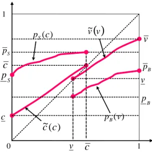
c, and sellers never propose anything above the highest acceptable price of buyers v. In other words, c pB(v) < ~v(v) and v pS(c) > ~c(c). Furthermore, in order for the marginal entrants to recover participation costs, we must also havec < vandc < v. Figure 2 visualizes the proposing and responding strategies of an equilibrium.

,

c v

( )

v

v

~

)

(

~

c

c

)

(

c

p

c

v

v

c

v

p

c

Figure 2: A non-full-trade equilibrium

3

Full-trade equilibria

The following important lemma gives participation conditions for the marginal types. Lemma 8 In any nontrivial steady-state equilibrium, p_B = pB(v), pB = pB(1), p_S =

pS(0), andpS=pS(c). Moreover,

`B( )(1 )~(p_B)(v p_B) = B (24)

`S( ) [1 ~ (pS)](pS c) = S: (25) In the left-hand sides of equations(24)and(25)in the lemma we have marginal traders’ expected pro…ts from trading, gross of participation costs, over a short period dt, divided by the length of the period. To see the intuition behind equation(24), note that a marginal participating buyer vmakes positive pro…t only if he meets a seller, proposes, and his o¤er is accepted (the combined probability is `B (1 ) ~(p_B)), and conditional on that, the pro…t is equal to the di¤erence between his valuation and the price he proposes, v p_B. Similar logic applies to equation(25).

There are two qualitatively di¤erent possibilities. First, it can be that at least one of the trading probabilities ~(p_B)or1 ~ (pS) is less than1. We call such an equilibrium a non-full-trade equilibrium because not every meeting results in a trade. The bargaining outcome in this class of equilibria is not ex-post e¢ cient, in the sense that there are buyer-seller pairs with positive matching surplus (i.e. v c > WB(v) +WS(c) or equivalently v~(v) >c~(c)) who do not trade when they meet. If, for example, ~(p

B)<1, then the buyers with types in a right-neighborhood of v do not trade with the sellers for whom ~c(c) ₂ (p_B; v]. An equilibrium of this kind is shown in Figure 2.

,

c v

( )

)

(

~

c

c

v

v

c

c

v

c

*

p

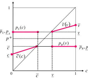
Figure 3: A full-trade equilibrium under take-it-or-leave-it o¤ering

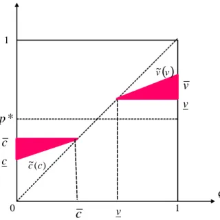
It may happen that the supports of the types in the market are separated, so that the marginal entrants trade with probability 1, i.e. ~(p_B) = 1 ~ (pS) = 1. We call such equilibria full-trade equilibria. Lemmas 7 and 8 imply that full-trade equilibria must have the following properties: (i) the supports for active buyers’types and active sellers’types are separate, i.e. v > c; (ii) the lowest buyer’s o¤er p_B is exactly at the o¤er acceptable to all active sellers, i.e. p

B =c; and (iii) the highest seller’s o¤erpS is exactly at the o¤er acceptable to all active buyers: pS =v. It is easy to see that the converse is also true. Thus we alternatively de…ne full-trade equilibrium to be a nontrivial steady-state equilibrium with p

B=cand pS =v. An example of such an equilibrium is shown in Figure 3.

A full-trade equilibrium admits a simple characterization. Conditions (24)and (25) of Lemma 8 take the form

`B( )(1 ) (v c) = B; (26)

`S( ) (v c) = S: (27)

Noticing that`S( )=`B( ) = , the entry equations(26) and(27)can be easily solved for and v c: = 1 S B z; (28) v c = B `B(z) + S `S(z) K(z): (29)

To complete the description of a full-trade equilibrium, note that in a steady state, the incoming ‡ow of active buyers must equal the incoming ‡ow of active sellers:

ζ

( )

(

) ( )

( )

Figure 4: Interpretation of z and K(z)

Sincev care determined,vandcare uniquely pinned down by(30). Full-trade equilibrium, if exists, is uniquely characterized by equations (26),(27), and (30).10

It is clear from(29)that K(z)<1is a necessary and su¢ cient condition for existence of a solution to equations (28) (30). The function

K( ) = B

`B( )

+ S

`S( )

will play an important role in our analysis. It can be interpreted as the expected par-ticipation cost incurred by a buyer-seller pair (i.e. B=`B( ) + S=`S( )) in a full-trade equilibrium until their meeting, if there is no discounting. A further insight about K(z)

is provided by the following lemma that will be used frequently in the proofs. The lemma shows that K(z) can be interpreted either as the following maximin value or the minimax value of adjusted accumulated participation costs until the next meeting.

Lemma 9 We have K(z) = max >0 min B (1 )`B( ) ; S `S( ) = min >0max B (1 )`B( ) ; S `S( ) :

Proof. Consult Figure 4. Note that`B( )is a nonincreasing function, while`S( )is an nondecreasing function. The maximin and minimax values are realized at the intersection of the curves

B (1 )`B( )

= S

`S( ) which occurs if and only if =z. Q.E.D.

1 0

Other endogenous variables are easily obtained. In particular, for v ₂ AB and c 2 AS, WB(v) = `B(z) r+`B(z)(v v),WS(c) = `S(z) r+`S(z)(c c), (v) = F(v) F(v) 1 F(v) and (c) = G(c) G(c).

But even if K(z) < 1, so that a solution to equations (28) (30) exists, it may not characterize an equilibrium, since buyers may have an incentive to bid higher than c, and similarly sellers may have an incentive to bid belowv. To rule out such deviations, we need additional conditions. Denote the virtual trader types as JB and JS:

JB(v) =v

1 F(v)

f(v) ; JS(c) =c+

G(c)

g(c)

Assuming that the virtual types are increasing functions, an assumption commonly made in the literature, we are able to show (in the Appendix) that the following necessary and su¢ cient conditions for a solution to equations (28) (30) to characterize a full-trade equilibrium: r min `B(z) (v c) max<sub>f</sub>c JB(v);0g ; `S(z) (v c) max_fJS(c) v;0g (31) r :

(If both denominators are 0, there is no upper bound so a full-trade equilibrium exists for allr 0.) Since the marginal typesvandcin a full-trade equilibrium do not depend on the discount rate r, we can see that these conditions will be satis…ed when r 0 is su¢ ciently small.

We are also able to show that a full-trade equilibrium is a unique equilibrium for small

r > 0. That is to say, there cannot be a non-full-trade equilibrium when r is small. The proof of this is based on the following lemma. This lemma proves that one important property of the full-trade equilibrium, that K(z) separate the entry gapv c (if any) and the length of the acceptance interval v c, carries over to all equilibria.

Lemma 10 In any nontrivial steady-state equilibrium, we have

v c K(z); (32)

v c K(z): (33)

The …rst inequality (32) is strict if r >0.

Proof. Sincec p

B < v v and v pS > c c;it follows from the entry conditions (24) and (25)that (1 )`B(v c) B; `S(v c) S; so that v c max B (1 )`B ; S `S K(z):

This proves (32). Ifr >0, we have v > v and c c, which make(32) strict. (33)is proved by applying a revealed-preference argument to the same entry conditions (24) and (25). Consider the deviations in which the v-buyers o¤er cand c-sellers o¤er v:

(1 )`B(v c) B;

, c v 0 1 1

)

(

v

p

( )

)

(

c

p

c

v

v

c

v

c

Figure 5: A full-trade equilibrium with too little entry

from which it follows that

v c min B (1 )`B ; S `S K(z): Q.E.D.

From Lemma 8, `BqB(v) B and `SqS(c) S, and these inequalities continue to hold for all participating types becauseqB (resp. qS) is nondecreasing (resp. nonincreasing) function. Lemma 5 then implies that the slopes of acceptance strategies are bounded from above as follows: ~ v0(v) r B+r ; ~c0(c) r S+r ; (34)

and therefore converge to 0as r_!0,

lim r!0v~

0_{(v) = lim} r!0c~

0_{(c) = 0: (35)}

Lemma 10 then implies thatv c and v c converge to a common limitK(z). Corollary 11 We have

lim

r!0(v c) = limr!0(v c) =K(z):

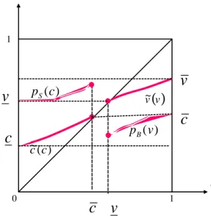
Now it is useful to introduce yet another level of equilibria classi…cation. A non-full-trade equilibrium may either have too much entry relative to the Walrasian benchmark,

v < c (as shown in Figure 2), or too little entry,v > c (as shown in Figure 5). Corollary 11 implies that a non-full-trade equilibrium with too much entry cannot exist whenr is small.

The proof that a non-full-trade equilibrium with too little entry cannot exist is based on the following idea (the details are in the Appendix.) As r _! 0, it follows from (35)

that the support of dynamic types narrows down to a singleton. Consequently, a marginal participating trader whose o¤er is in the interior of the support of the bargaining partner gains relatively little vis-a-vis proposing at the boundary of the support (i.e. seller o¤ering

v and buyer o¤ering c), but risks a substantially reduced probability of trading. We are able to show that bidding the endpoint of the support is the dominant choice, so for small

r it must be that p

B =c and pS =v. We therefore have proven the following uniqueness result.

Proposition 12 (Existence and uniqueness of full-trade equilibrium) If K(z) <

1, then r > 0 exists such that for all r ₂ [0; r] there is a unique equilibrium and it is full-trade.11

De…ne Walrasian pricep as the price that clears the ‡ows of the arriving cohorts:

b[1 F(p )] =sG(p );

It is immediate from the characterizing equations (28) (30) that full-trade equilib-ria converge to perfect competition as the frictions of time discounting and participation cost are removed.12 Speci…cally, the marginal participating types converge to p and the acceptance interval (and hence the price interval) converges to _fp _g. Since full-trade equi-libria are the only equiequi-libria when r is small, it also follows that all equilibria of our model converge to perfect competition. We state this as a corollary.

Corollary 13 (Convergence to perfect competition) As the frictions of participation cost and discounting are removed, all equilibria of our model converge to perfect competition, i.e. lim ( B; S)!0 lim r!0v = ( Blim; S)!0 lim r!0c=p ; lim ( B; S)!0 lim r!0 [c; v] = ( Blim; S)!0 lim r!0[pB; pS] =fp g:

When r > r , then a full-trade equilibrium does not exist. Note that it is possible that

r =₁ so that a full-trade equilibrium exists for allr. This may happen (as our example shows) when the search costs B and S are so large (but not larger than K(z)) that the entry gap is v c is su¢ ciently large so that both c JB(v) < 0 and JS(c) v < 0 and therefore from (31), r = ₁. On the other hand, it can also happen that r < ₁

so that a full-trade equilibrium does not exist for large r. We can easily see that this will happen if the search costs B; S are su¢ ciently small. Even stronger, we can show that lim( B; S)!0r = 0.

1 1_{Recall that for expositional simplicity we have assumed that the types are distributed on[0;1]. If the}

support were [a1; a2], then the condition would readK(z)< a2 a1.

κ * r 6 / 1 1/2

Figure 6: The values ofr and for which a full-trade equilibrium exists in example 14 are shown by the shaded area

In a full-trade equilibrium, the entry gapv c=K(z), so thatlim( B; S)!0(v c) = 0.

Because both v and c converge to the Walrasian price p , it follows that JB(v) ! p (1 F(p ))=f(p ) and JS(c)!p +G(p )=g(p ). Consequently,

c JB(v) ! (1 F(p ))=f(p );

JS(c) v ! G(p )=g(p ); and it follows from (31) that as( B; S)!0,

r v c !min `B(z)f(p ) 1 F(p ) ; `S(z)g(p ) G(p ) :

Consequently, lim( B; S)!0r = 0, so that given any r > 0, a full-trade equilibrium does

not exist when the search costs B; S are su¢ ciently small. An example may help understand these points better.

Example 14 Buyers and sellers are born at the same rate, which is normalized to be 1, i.e. b = s = 1. The values and costs are uniform [0;1] distributed, i.e. F(v) = v,

G(c) = c. The bargaining power is evenly distributed, i.e. = 1=2; and the search costs of buyers and sellers are also the same: S = B . The matching function is given by M(B; S) = min_fB; S_g (so that all traders who are searching at a given point in time are matched at the arrival rate 1 in this symmetric setting). One can check that the entry gap in a full-trade equilibrium is given by v c= 2 and the condition (31) takes the form

r 2 =max_f0:5 3 ;0_g. A non-trivial equilibrium only exists if the entry gap is less than 1, i.e. 2 <1. The values ofr and for which a full-trade equilibrium exists are shown in Figure 6.

We collect all these …ndings in a theorem below, the formal proof of which is in the Appendix.

Theorem 15 Assume that the virtual types JB(v) and JS(c) are increasing functions of their arguments. Then a full-trade equilibrium exists if and only if K(z) < 1, in which case there exists a unique solution to the characterizing equations (28) (30), and r r

where r is given by (31). Moreover, an r > 0 exists such that a full-trade equilibrium is the unique equilibrium of the model for r ₂ [0; r]. If, on the other hand, r > r , then a full-trade equilibrium does not exist. In particular, given any r > 0, a > 0 exists such that a full-trade equilibrium does not exist whenever B, S < .

4

Necessary and su¢ cient condition for no market

break-down

It is not hard to see that the conditionK(z)<1, a necessary condition for the existence of a full-trade equilibrium, is also necessary for existence of any nontrivial equilibrium of our model. Indeed, it is trivial if r = 0, in which case any nontrivial equilibrium is full-trade. On the other hand, ifr >0and some nontrivial equilibrium exists, then Lemma 10 together with v c 1 implies the conditionK(z)<1.

Perhaps surprisingly, the condition K(z) <1 is also su¢ cient for existence of a non-trivial equilibrium of our model.

Theorem 16 (No market breakdown) A necessary and su¢ cient condition for exis-tence of a nontrivial equilibrium is that K(z)<1.

Taken together with the last statement of Theorem 15, Theorem 16 implies that a non-full-trade equilibrium exists if r is su¢ ciently large and participation costs are su¢ ciently small.

Corollary 17 (Existence of a non-full-trade equilibrium) > 0; r > 0 exist such that a non-full-trade equilibrium exists whenever r > r and B, S< .

This section is devoted to the main elements of the proof of Theorem 16. Our goal is to prove that there exists a tuple (pB; pS;v;~ ~c; B; S; B; S; ; ) of strategies, steady-state distributions and steady-state masses of traders, that satis…es our mathematical de…nition of nontrivial equilibrium of the take-it-or-leave-it o¤ering model. However, in order to apply the …xed point theorem to do our job, it is much better to transform and reduce our space of equilibrium objects. De…ne NB : [0;1] ! R+ and NS : [0;1] ! R+ as the

steady-state unnormalized distributions of buyers and sellers, i.e. NB(v) B (v) and

NS(c) S (c). Then we will take the tuple of payo¤s and unnormalized distributions (WB; WS; NB; NS) E as the primary con…guration of equilibrium objects.

Indeed, our mathematical de…nition of a nontrivial equilibrium can be regarded as a …xed point of some mapping T that brings an initial con…guration E= (WB; WS; NB; NS) (from some appropriate domain) to a new con…guration E = (W_B; W_S; N_B; N_S). This mapping is de…ned as follows. First, we let

B =NB(1); S =NS(1); (v) = NB(v) B ; (c) = NS(c) S ; = B S: (36)

Then determine the dynamic types (~v;~c) according to(1) and (2), and their distributions

~_;~ _{according to(3)and(4). Next, we determine the best-response proposing strategies} (pB; pS) according to (5) and (6), but whenever there are multiple best-responses, we use the maximal response for buyers and the minimal for sellers:

pB(v) = sup arg max

2[0;1]~( )[~v(v) ] (37)

pS(c) = inf arg max

2[0;1][1 ~ ( )][ ~c(c)] : (38)

Having de…ned the proposing strategies, we can de…ne and the expected pro…ts ( B; S) in a given meeting according to(7)and(13), as well as the probabilities of trading(qB; qS) according to (8)and(14). With those at hand, we can recover the resulting lifetime payo¤s through their corresponding recursive equations, (11)and (16):

W_B(v) = max_fRB( )[ B(v) + (1 qB(v))WB(v)] KB( );0g (39)

W_S(c) = max_fRS( )[ S(c) + (1 qS(c))WS(c)] KS( );0g: (40) After that, we determine the best-response entry strategies as in (12)and (17), and …nally determine the resultant steady-state distributions of types according to:

N_B(v) = Z v 0 B(x)b `B( )qB(x) dF(x); N<sub>S</sub>(c) = Z c 0 S(x)s `S( )qS(x) dG(x): (41) In the Appendix, some additional details and quali…cations are provided to guarantee that this mapping is well-de…ned.

Our existence proof will be based on the Schauder …xed point theorem, which asserts that: if D is a nonempty compact convex subset of a Banach space andT is a continuous function from D toD, thenT has a …xed point.

In order to make this theorem applicable, certain details need to be taken care of. The main di¢ culty is we need to make sure that as we apply the mapping T, we do not lose positive entry. To deal with this potential complication, we …rst prove existence of what we call an "-equilibrium, which is an actual equilibrium in a "-model in which positive entry always occurs because of an outside subsidy.

We modify our original model in three ways. Firstly, we add a subsidy that ensures that all buyers with typev 1 "and all sellers with typec "enter. In particular, every new-born trader is quali…ed to received a ‡ow of subsidy for her market participation, provided that (i) her type satis…es v 1 " orc ", and (ii) she would choose not to participate if no subsidization is available. Further, the ‡ow rate of the subsidy for a quali…ed trader would be the least amount that is enough to make the trader voluntarily participate. That is, for example, a new-born buyer with type v 1 " and `B( ) B(v) < B( ) will, conditional on entry, receive a ‡ow amount B( ) `B( ) B(v) per unit of time so that she is indi¤erent between entering or not. (We assume traders enter whenever indi¤erent.) Hence the entry conditions (12) and (17)are changed as:

B(v) = I[`B( ) B(v) B orv 1 "] (42) S(c) = I[`S( ) S(c) S orc "]: (43)

Because any subsidized traders are simply indi¤erent between entering or staying out, our equations for payo¤s WB, WS, and bargaining strategies v~, ~c, pB, pS do not need to be changed.

Although we now have a positive lower bound for the in‡ows of traders, we have not had a positive lower bound for the mass of traders in the market because the out‡ow rate (i.e. `B( )qB(v) or `S( )qS(c)) could be potentially very large. Concerned with this, we impose the second modi…cation, which ensures that the buyers’arrival rate `B( ) and the sellers’arrival rate`S( )are bounded by`Band`S. Speci…cally, given the original matching function M(B; S), we replace it with a new one M~(B; S) de…ned as:

~

M(B; S) = min M(B; S); B`B; S`S : (44) Notice that M~ has all the properties as a matching function as long as M has. But now we make sure that

`B( ) `B; `S( ) `S: (45) While the …rst two modi…cations are added to make the mass of traders bounded from below, we also want it to be bounded from above, because our domain D need to be compact. It su¢ ces to have a lower bound for the out‡ow rate (`B( )qB(v)or`S( )qS(c)). For a type who chooses to enter without subsidization, there is naturally an upper bound for its mass because her expected trading surplus must be larger than her participation cost. More precisely, for an unsubsidized participating v-buyer,`B( )qB(v) `B( ) B(v) B. However, a subsidized buyer could have `B( )qB(v)< B. Concerned with this, our third modi…cation is, we disqualify subsidized traders in a way that ensures the out‡ow rates of subsidized types are at least Bor S. In particular, the disquali…cation is a Poisson process, where the Poisson rate (which is contingent on type) is the least one that makes the out‡ow rate not lower than the lower bound B or S. That is, for example, a currently quali…ed

v-buyer with `B( )qB(v) < B will be disquali…ed and exit immediately at a Poisson rate B `B( )qB(v); while a currently quali…ed v-buyer with `B( )qB(v) B will not be disquali…ed. Notice that for any type, either subsidized or unsubsidized, a v-buyer’s gross out‡ow rate must bemax<sub>f</sub>`B( )qB(v); Bg. Therefore, the steady-state equations(41) are simply changed as:

N_B(v) = Z v 0 B(x)b max_f`B( )qB(x); Bg dF(x) (46) N<sub>S</sub>(c) = Z c 0 S(x)s max<sub>f</sub>`S( )qS(x); Sg dG(x): (47) It completes the descriptions of our "-model.

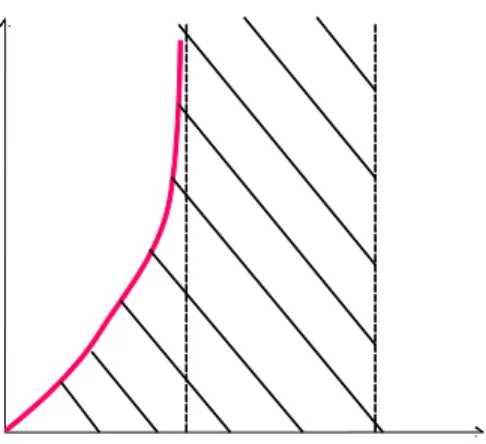
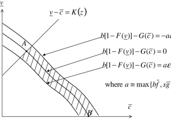
In the Appendix, we show that our"-model has at least one equilibrium, which we shall call an"-equilibrium. Next, we prove that if" >0is su¢ ciently small, then an"-equilibrium is a true equilibrium of our model (this is Proposition 24 in the Appendix). The main idea of the proof can be illustrated graphically, see Figure 7.

First, as in Lemma 10, we show that in"-equilibrium also, we must havev c K(z). Second, we show that the trading ‡ows are almost balanced, the discrepancy bounded in absolute value by (a multiple of) ". Imposing these constraints on the set of values

c

( )

( )

Figure 7: c > "and v <1 "for small "

graph makes clear, the shaded area collapses to the curvilinear segmentAB. Consequently, as " gets arbitrarily small, the minimal c in the shaded area is arbitrarily close to the horizontal coordinate of point A, and the maximal feasible v is arbitrarily close to the vertical coordinate of A. It follows that for small enough" >0, the constraintsc > " and

v < 1 " become non-binding and the "-equilibrium becomes a true equilibrium of our model.

5

Comparison to the full information model of Mortensen

and Wright (2002): private information may enhance

wel-fare

Mortensen and Wright (2002; MW) consider a model that di¤ers from ours only in one respect: MW assume full information, i.e. bargainers know each other’s type. Consequently, proposers hold their partners to their reservation values (i.e., to their dynamic types), and the proposing strategies depend on both the trader’s and his partner’s type. In other words, for the buyers, the proposing strategy is pB(v; c) = ~c(c), if c~(c) v~(v), while it can be de…ned as any price less than ~v(v) if ~c(c) < ~v(v) (such a price will be rejected by the seller). Similarly, pS(v; c) = ~v(v)ifc~(c) ~v(v).

Even though there is no private information, not every meeting may result in a trade because it may be that ~v(v)<~c(c), so that the pair does not trade. But the same way as in our model, MW show existence of a full-trade equilibrium if r is su¢ ciently small (i.e., our Proposition 12 also holds assuming full information). Comparing their conditions for existence of a full-trade equilibrium, they show that, similar to our model, there is an upper bound such that a full-trade equilibrium exists if and only if the discount rate is below that bound. Unlike in our model, however, the bound is always binding (i.e. less than in…nity). MW also suggest (but do not prove) that a non-full-trade equilibrium may exist.

,

c v

v

c

c

*

p

( )

Figure 8: When types are publicly known, marginal participating types extract full rents from their partners

in particular the necessary and su¢ cient condition for existence of equilibrium (the no market breakdown condition) in a model with full information is the same as in our model:

K(z) < 1.13 The proof is even easier because we do not have to consider proposing strategies in our construction of the best-response mapping T. The only change in the de…nition of T is that the expected pro…ts and trading probabilities are now

B(v) = (1 ) Z ~ v(v) ~c(c) [v ~c(c)]d (c); qB(v) = Z ~ v(v) ~c(c) d (c) S(c) = Z ~ v(v) ~c(c) [~v(v) c]d (v); qS(c) = Z ~ v(v) ~c(c) d (v) instead of (7),(8),(13) and (14).

The equilibrium in both models is unique for small r 0.14 This makes it feasible to compare the levels of social welfare under private and public information for such values of

r. The marginal participating types v and c in the full-trade equilibria are equal in both models only whenr= 0. Whenr increases away from0, our marginal types do not change, while as MW show they move towards each other in their model. In other words, under complete information there is entry by extramarginal types.

To understand why this is so, note that, unlike in our model, under full information the marginal types extract full rents from the partners to whom they propose (see Figure

1 3

The details of the proof are available on request.

1 4

MW do not prove existence of a non-full-trade equilibrium in their model. We …ll this gap by showing the changes that would be necessary to our existence proof to cover the case of public information.

8). In contrast, our marginal types are only able to extract the rents of the most ine¢ cient partner type. As r increases away from0, the distributions of the dynamic types become, ceteris paribus, more heterogeneous, and consequently there are more rents to be had by the marginal types. This creates incentives for the extramarginal types to enter. There are no such incentives in our model.

In the presence of matching externalities, more entry may or may not be socially desir-able. Under private information, the slope of the welfare Wp(r) as a function ofr is

dWp(0) dr = W_B0 `B(z) W<sub>S</sub>0 `S(z) (48) where W_B0 b Z 1 v (v v)dF(v); W_S0 s Z c 0 (c c)dG(c): (49) This is simply the direct e¤ect of discounting. In particular, the e¤ect of discounting on buyers’ (resp. sellers’) welfare is proportional to their expected waiting time 1=`B (resp. 1=`S).

Under full information, on the contrary, the slope of the welfare Wf(r) as a function of r, as shown in the Appendix, is

dWf(0) dr = W_B0 `B(z) W<sub>S</sub>0 `S(z) sG(c) [ _{B B}(z) _{S S}(z)] 0(0) (50) where 0(0)is the derivative d_dr under full information evaluated atr= 0, and _B( )(resp. S( )) is the absolute value of the derivative of buyers’ expected waiting time 1=`B( ) (resp. 1=`S( )) with respective to , i.e.

B( ) d d 1 `B( ) >0; <sub>S</sub>( ) d d 1 `S( ) >0:

Other than the direct e¤ect, the increase in r away from 0, by inducing additional entry, could increase or decrease the buyer-seller ratio , which in turn a¤ects the expected waiting time1=`Band1=`S by (in …rst order) B(z)and S(z)respectively. Thus the indirect e¤ect on the total accumulated participation costs incurred by a cohort is the last term in (50).

In the Appendix, we also show that the di¤erence of the two slope can be written as

dWp₍₀₎ dr dWf₍₀₎ dr = sG(c) [ B B(z) S S(z)] 0₍₀₎ = [ S(z) ] W_S0 `S(z) W<sub>B</sub>0 (1 )`B(z) (51) where S( ) 1 m0( )=m( ) is the elasticity of the matching function with respect to the mass of sellers (i.e. S( ) = SM2(B; S)=M(B; S)). It is easy to see that this slope

may be either positive or negative, depending on the elasticity of the matching function as well as original welfare shares of buyers and sellers. Recall that we have shown that there is more entry for small r in the full-trade equilibrium of MW. The extramarginal sellers who enter impose a negative externality on the inframarginal sellers and a positive externality

on the inframarginal buyers. A symmetric statement applies to the extramarginal buyers who enter. The positive and negative externalities completely cancel out only when the Hosios (1990) condition, i.e. S = holds, in which case we have dW

p₍₀₎ dr =

dWf(0)

dr . If, for example, the elasticity S is larger than sellers’bargaining weight , and if the original share of sellers’welfareW_S0 is large (relative toW_B0) so that the last term in(51)is positive, then the welfare under private information is larger than under full information.

We formulate these …ndings in a proposition.

Proposition 18 For all su¢ ciently small r > 0, the private information welfare Wp(r) is either greater or smaller than the full information welfare Wf_{(r), depending on whether} the right-hand side of (51) is positive or negative.

6

Related literature and concluding remarks

Most related to our paper is the recent note by Lauermann (2006b), which we believe was concurrently written. He also asks the question: can private information be welfare-enhancing in dynamic matching and bargaining models, and arrives to the same conclusion that it can, but for a very di¤erent reason and in a quite di¤erent model. There is no cost of search, and all potential traders enter. There is no discounting either. The only friction is exogenous exit rate .15 _{The sellers have all the bargaining power, = 1, and}

all have the same cost normalized to 0. As in our model, the buyers are heterogeneous. Lauermann (2006b) considers both private and full information. He shows that, as the friction is removed ( _! 0), with private information all equilibria converge to perfect competition. In particular, the price o¤ers converge to the sellers’cost, i.e. to 0.

In marked contrast, with full information the price o¤ers stay bounded away from 0

even as _! 0. The reason why this happens is the following. When sellers know buyers’ valuations, they are able to extract all the surplus from the buyers, by o¤ering the price equal to the buyer’s valuation, perhaps a penny below. When a seller meets a buyer, she knows that she can guarantee at least the average buyer’s valuation _E(v) in the next meeting. Lauermann (2006b) shows that _E(v)is bounded away from 0as _!0. Since no seller will o¤er a price less than(1 )_E(v), it follows that the buyers with valuations below

(1 )_E(v)will never trade. Since e¢ ciency here means that sellers should trade with all buyers, this outcome is clearly less e¢ cient with full information. Lauermann (2006b) also shows that having exogenous exit is necessary for this e¤ect to occur. Extreme bargaining power is also necessary; it is an open question whether seller heterogeneity could be allowed. While the entry-deterrent e¤ect of private information has not, to our knowledge, been considered in the dynamic matching and bargaining literature, this literature is quite large and there is a number of related papers. The great majority of papers have assumed full information: Mortensen (1982), Rubinstein and Wolinsky (1985), Rubinstein and Wolinsky (1990), Gale (1986), Gale (1987) and Mortensen and Wright (2002). The …rst paper to look at convergence in a setting with private information is the un…nished manuscript of

1 5

The model is therefore similar to Satterthwaite and Shneyerov (2005), the main di¤erence being that Satterthwaite and Shneyerov (2005) consider multilateral meetings in which sellers run auctions among the buyers they are matched with, whereas matching is strictly bilateral in Lauermann (2006b).

Butters (1979). Other papers that have incorporated private information in some form are Wolinsky (1988), De Fraja and Sakovics (2001) and Serrano (2002).

Recently, there has been a resurgence of interest in this topic: Lauermann (2006a), Sat-terthwaite and Shneyerov (2007), Atakan (2007). The focus of these papers is convergence to perfect competition.16 This is also the focus of large but less related literature on sta-tic double auctions, beginning with Chatterjee and Samuelson (1983) and Wilson (1985), followed by, among others, , Gresik and Satterthwaite (1989), Satterthwaite and Williams (1989), Satterthwaite (1989), Williams (1991), Rustichini, Satterthwaite, and Williams (1994), and more recently Satterthwaite and Williams (2002), Tatur (2005), Cripps and Swinkels (2005), Reny and Perry (2006), Fudenberg, Mobius, and Szeidl (2007). Wu (2005) studies a double auction with a small entry cost.

Given that search costs may lead to market breakdown, existence of a non-trivial equi-librium is in general not guaranteed. The literature to date has only provided existence results when search costs are small. Satterthwaite and Shneyerov (2007), for example, study a bilateral matching and bargaining model with two-sided private information in which sell-ers run auctions among the buysell-ers whom they are matched with, and show existence for small search costs. Atakan (2007) has provided an important extension of Satterthwaite and Shneyerov (2007) to multiple units, and shows existence again only for small frictions.17

We, on the other hand, derive a necessary and su¢ cient condition for existence (i.e. for no market breakdown) when frictions are arbitrary.

All these …ndings call for future research. Can our results be generalized to double auctions? Even more interesting would be to identifying the set of bargaining mechanisms for which private information may be welfare-enhancing. One di¢ culty would be to prove uniqueness of a full-trade equilibrium. For this, it might be fruitful to combine our approach with that of Lauermann (2006a) who develops techniques for studying general dynamic matching and bargaining markets.

1 6_{In addition, Hurkens and Vulkan (2006) study the role of privately observed deadlines in a matching}

and bargaining market.

1 7_{Alternatively, he is able to show existence in general, but assuming that there is costless entry in the}

Appendix

Proof of Lemma 3: We prove the results for buyers only. Rewrite the recursive equation for the buyers:

WB(v) = max n RB[ ^B(v; pB(v);v~(v)) + (1 q^B(pB(v);v~(v)))WB(v)] KB;0 o = max RBmax ; [ ^B(v; ; ) + (1 q^B( ; ))WB(v)] KB;0 = max RBmax ; [ ^B(v WB(v); ; ) +WB(v)] KB;0 :

where ^B(v; ; ) and q^B( ; ) are conditional on proposing and adopting acceptance level : ^_{B(v; ; ) (1 )}Z ~ c(c) [v ]d (c) + Z pS(c) [v pS(c)]d (c) (52) ^ qB( ; ) (1 ) Z ~ c(c) d (c) + Z pS(c) d (c): (53)

If RB = 1 (or r = 0), the recursive equation indicate that whenever WB(v) 6= 0, we have max ; ^B(v WB(v); ; ) =KB >0 so that v WB(v) must be some positive constantx. It is then easily seen that the recursive equation has a unique solutionWB(v) = max_fv x;0_g, which is nondecreasing, continuous and convex.18

Now suppose RB < 1 (or r > 0). Then the right-hand side of the recursive equation can be regarded as a contraction mapping that assigns each WB another function on the same domain. Applying standard techniques of discounted dynamic programming, we can see that the solutionWB is unique, nondecreasing, continuous and convex.

From the continuity and monotonicity, WB(v) is absolutely continuous and hence dif-ferentiable almost everywhere. Whenever di¤erentiable, we have

W_B0 (v) = _B(v)RB qB(v)[1 WB0(v)] +WB0 (v) : Solve for W_B0 (v), W_B0 (v) = B(v)RBqB(v) 1 _B(v)RB[1 qB(v)] = B(v)RBqB(v) 1 RB[1 qB(v)] = _B(v) `BqB(v) r+`BqB(v) :

Forv₂AB, the trading probabilityqB(v)must be strictly positive, otherwise the participa-tion cost Bcannot be recovered. ThusWB(v)is strictly increasing onAB andAB = [v;1].

1 8_{Ifv x <0thenW}

B(v)cannot bev xand henceWB(v) = 0. Ifv x >0thenWB(v)cannot be 0 because the …rst maximand atWB(v) = 0is

max

In order to prove 20, it now su¢ ces to show WB(v) = 0. Indeed, if WB(v) 6= 0, then either v = 0 or v = 1. We preclude the possibility of v = 1 because we are looking at nontrivial equilibrium. v = 0 is also impossible because in that case type 0 buyer cannot expect their participation cost recovered. Q.E.D.

Proof of Lemma 5: From lemma 3, v~(v) and c~(c) are absolutely continuous. Their derivatives, which exist almost everywhere on AB and AS, are given by

~ v0(v) = r r+`BqB(v) 0 and ~c0(c) = r r+`SqS(v) 0:

Moreover, the above inequalities are strict if and only if r >0. Q.E.D. Proof of Lemma 7:

Step 1: p_S v and pB c. Suppose p

S < v. Then there is some active seller with type c proposing pS(c) < v. Then her o¤er will be accepted with probability one and she can raise her o¤er without a¤ecting this probability. We get the desired contradiction and havep_S v. Similar logic with a buyer considered would show pB c.

Step 2: c < v and c < v.

Suppose v c. Then buyer with type v cannot recover the participation cost. It is because (i) when she is the proposer, she cannot get any surplus since her value v is not higher than the lowest price cacceptable by any seller; and (ii) when she is the responder, again she cannot get any surplus since, from step 1, her value v is not higher than the lowest price p

S proposed by any seller. We get the desired contradiction and havec < v. Similar logic with a cseller considered would show c < v.

Step 3: For allc₂[0; c]and allv₂[v;1],~c(c)< pS(c) pS v and c p_B pB(v)< ~

v(v).

Fix any c ₂ [0; c]. Fromc < v in step 2, we have max

nh 1 ~ ( ) i [ ~c(c)] o > 0. (For example, the seller can propose(c+v)=2.19) Therefore, we have1 ~ (pS(c))>0and

pS(c) c~(c)>0. Notice that 1 ~ (pS(c))>0 implies pS v. It completes the proof of the …rst part of this step. The second part is shown by symmetric logic.

Now we have already provedv p_S pS v andc p_B pB c. If r= 0, then by lemma 5, we have v=v andc=c, and hence it proves our claims forr = 0case. Ifr >0, then again by lemma 5, then v~( ) and ~c( ) are strictly increasing. Then 1 ~ (pS(c))>0 (resp. ~(pB(v))>0) implies pS < v (resp. p_B > c). It proves our claims forr > 0 case. Q.E.D.

Proof of Lemma 6: If r = 0, then from Lemma 7, pB(v) and pS(c) are constant on

AB and AS respectively. The rest of this proof consider the case where r >0.

Consider a buyer with typev v. Recall (5) and by standard argument, we have

h

~(pB(v2)) ~(pB(v1)) i

[~v(v2) ~v(v1)] 0:

From Lemma 5, ifr >0, thenv~(v) is strictly increasing, thus ~(pB(v))is nondecreasing in

v. Now suppose v1 < v2 butpB(v1) > pB(v2). Since ~(pB( ))is nondecreasing, we have

1 9 _{and have positive densities on [v;1]and [0; c]because F andG have. Then ~ and ~ also have}

~(pB(v1)) ~(pB(v2)). On the other hand, ~( ) is nondecreasing, we have ~(pB(v1))

~(pB(v2)). Therefore ~(pB(v1)) = ~(pB(v2)). Then either ~(pB(v1)) = ~(pB(v2))>0 or

~(pB(v1)) = ~(pB(v2)) = 0.

Suppose …rst that ~(pB(v1)) = ~(pB(v2))>0. Then typev1 buyers could o¤er a lower

price, namely pB(v2), without a¤ecting the probability of being accepted, which is positive.

We get a contradiction.

Now suppose ~(pB(v1)) = ~(pB(v2)) = 0. Then max n

~( )[~v(v) ]o = 0 for v =

v1; v2. But by Lamma 5 and Lamma 7, v v imply ~v(v) v > c. Then above objective

function can be guaranteed to be strictly positive by setting = (v+c)=2. Again we get a contradiction. Therefore, pB(v) are nondecreasing.

Using symmetric logic, we can prove corresponding results for the sellers’side, namely,

pS(c) are nondecreasing. Q.E.D.

Proof of Lemma 8: The claims in the …rst sentence are straight implications of Lemma 6. For the rest, notice that by Lamma 7, v p

S and therefore the v buyer will make positive pro…t only when he is the proposer. His o¤erp_B will be accepted only if the seller’s dynamic type ~c(c) p_B. The entry condition(12) then implies(24). Similar logic leads to(25). Q.E.D.

Proof of Proposition 12: For concreteness, focus on the sellers (a symmetric argu-ment applies for the buyers). Since equilibrium proposing strategy is nondecreasing, it is su¢ cient to rule out a deviation to a higher bid > v for the sellers with type c. The expected pro…t in a given meeting is

S(c; ) = ( c) 1 ~ ( ) ; and its slope is

@ S(c; )

@ = 1 ~ ( ) ( c) ~

0_{( ) (54)}

= ~0( )hJ~B( ) c

i

whereJ~B( )is the “virtual type”that corresponds to the distribution of dynamic types ~, ~

JB( )

1 ~ ( ) ~0_{( )} :

Given that the dynamic type ~v(v)in a full-trade equilibrium is a linear function which can be calculated as

~

v(v) = rv+`Bv

r+`B

;

straightforward algebra shows that

~ JB( ) = r r+`B JB r+`B r `B r v + `B r v ; (55)

where JB(v) is the virtual type function for the distribution F. Substituting(55) in the slope formula (54), we obtain

@ S(c; ) @ = ~ 0_{( )} r r+`B JB r+`B r `B r v + `B r v c (56)

Clearly, a deviation to < v is not pro…table, so we only need to consider > v. A necessary condition for such a deviation to be not pro…table is that @ S(c; )=@ 0 at = v, i.e. the expression in the brackets on the right-hand side of equation (56) is non-positive when =v. This is also su¢ cient because of the monotonicity of JB. This gives the inequality

rJB(v) +`B(z)v

r+`B(z)

c 0:

Similarly, a necessary and su¢ cient condition to rule out a pro…table deviation by a buyer with type v is

v `S(z)c+rJS(c) r+`S(z)

0:

Equivalently, we can eliminate rfrom both inequalities to obtain(31), the upper bound on

r in text.

Proof that a non-full-trade equilibrium with too little entry cannot exist for smallr >0: Since o¤ering strategies are increasing, it is su¢ cient to rule out the deviations by marginal participating buyers and sellers. Consider a type c seller who deviates by o¤ering > v in all meetings. His expected payo¤ in a given meeting

S(c; ) = ( c)

h

1 ~ ( )i;

with the slope

@ S(c; )

@ = 1 ~ ( ) ( c) ~ ( ); (57)

where ~ is the density of buyers’dynamic types. This density is equal to

~ ( ) = ~0_{( ) =} (v( )) ~

v0_{(v( ))}

where is the density of buyer types in the market and v( ) is the inverse of ~v(v), i.e.

~

v(v( )) = . From (34) in text, for allv v,v~0(v) r=(r+ B), so we have ~ ( ) 1 + B

r (v( )): (58)

We now derive a lower bound on the endogenous density of buyers’types . From the steady-state condition, we can deduce

(v) = bf(v) M(B; S)qB(v) bf(v) M(B; S): (59) and B = Z 1 v bf(v)dv `BqB(v) b B [1 F(v)]; (60)

where the last inequality follows from the fact that the v-type buyer must recover his participation cost,`BqB(v) B. Corollary 11 and the steady-sta