CorClustST - Correlation-based Clustering of Big
Spatio-Temporal Datasets
Marc H¨uscha,∗, Bruno U. Schyskab, Lueder von Bremenb
aTU Dortmund, Fakult¨at Statistik, 44221 Dortmund, Germany
bCarl von Ossietzky Universit¨at Oldenburg, ForWind, 26129 Oldenburg, Germany
Abstract
Increasing amounts of high-velocity spatio-temporal data reinforce the need for clustering algorithms which are effective for big data processing and data reduc-tion. As currently applied spatio-temporal clustering algorithms have certain drawbacks regarding the comparability of the results, we propose an alternative spatio-temporal clustering technique which is based on empirical spatial cor-relations over time. As a key feature, CorClustST makes it easily possible to compare and interpret clustering results for different scenarios such as multi-ple underlying variables or varying time frames. In a test case, we show that the clustering strategy successfully identifies increasing spatial correlations of wind power forecast errors in Europe for longer forecast horizons. An extension of the clustering algorithm is finally presented which allows for a large-scale parallel implementation and helps to circumvent memory limitations. The pro-posed method will especially be helpful for researchers who aim to preprocess big spatio-temporal datasets and who intend to compare clustering results and spatial dependencies for different scenarios.
Keywords: Clustering, Big Spatio-Temporal Data, Spatial Dependence,
Preprocessing, Data Reduction
∗Corresponding author
Email addresses: [email protected](Marc H¨usch),
[email protected](Bruno U. Schyska),[email protected](Lueder von Bremen)
1. Introduction
Due to the continuing growth of data in many areas of application, there is an urgent need for efficient machine learning and data mining algorithms that can identify patterns in massive datasets. Clustering algorithms [1, 2, 3] are a popular tool to systematically detect groups of objects that share similar
5
characteristics and can help to preprocess, reduce and compress big datasets. Especially in environmental applications, data is often available in high fre-quency across space and time which leads to special requirements for clustering methods to identify objects that are similar regarding both dimensions. The
most popular clustering algorithms like thek-means algorithm [4] or
hierarchi-10
cal clustering algorithms [5, 6, 7] were, however, not developed specifically for spatio-temporal data and they do not take the special characteristics of such data into account. It is therefore important to develop novel spatio-temporal clustering algorithms which are able to efficiently extract information from big spatio-temporal datasets. In this sense, Kisilevich et al. (2010) [8] published a
15
survey which gives an overview of common spatio-temporal clustering methods and applications. Most of the methods that are currently employed for clus-tering spatio-temporal data are based on density-based clusclus-tering techniques. DBSCAN [9], for instance, scans the entire data and marks each point as a core object (objects located in a cluster), border object (objects located at the border
20
of a cluster), or noise (objects that are not located in a cluster) by determining the number of objects that are within a certain distance around each object. Birant and Kut (2007) [10] extended the idea of DBSCAN for spatio-temporal data. Their algorithm ST-DBSCAN marks each object based on the number of objects that are within a certain spatial and a certain temporal distance.
25
More recently, Agrawal et al. (2016) [11] developed a spatio-temporal cluster-ing strategy which bases on the density-based clustercluster-ing algorithm OPTICS (Ordering Points to Identify the Clustering Structure) [12]. Their proposed strategy ST-OPTICS first orders the observations in a dataset, then clusters them with a modified version of ST-DBSCAN and finally merges the resulting
micro level clusters with an agglomerative algorithm. The authors showed in an application that the proposed strategy can lead to better clustering results than ST-DBSCAN in terms of cluster validity.
Despite considerable progress in the field of spatio-temporal clustering in recent years, currently applied methods still have some drawbacks that
rein-35
force the need for alternative spatio-temporal clustering algorithms: Compared
to thek-means algorithm, ST-DBSCAN and ST-OPTICS have the advantage
that the number of clusters does not have to be predefined. One drawback of these algorithms is, however, that they do not directly find meaningful cluster centers which represent a certain cluster. This can be uncomfortable for a
fur-40
ther analysis of cluster interconnections and especially for the purpose of big data reduction. In addition, the control parameters of these clustering algo-rithms need to be tuned in order to achieve an optimal clustering solution with respect to certain optimization criteria. In case of different control parameters, clustering results for different scenarios (e.g. varying time frames or multiple
45
underlying variables) are, however, difficult to compare.
The considerations above have led to a novel approach for clustering big spatio-temporal datasets: By computing empirical correlations between pairs of spatial points over time, it is possible to find clusters that are easier to interpret, regardless the number of time points and the underlying variable used in the
50
analysis. As spatio-temporal data is often positively correlated only up to a certain spatial distance, it is not necessary to compute correlations for all pairs of points. By considering only those objects that are located within a certain spatial distance, the computation time and the memory requirements of the clustering technique are reduced drastically. CorClustST takes up some basic
55
ideas of ST-DBSCAN and ST-OPTICS but provides a new concept in order to achieve a better comparability of clustering results for different scenarios. The applicability of the algorithm is exemplified with a cluster analysis of wind power forecast errors in Europe for different forecast horizons. It turns out that the algorithm successfully manages to represent increasing spatial correlations
60
This paper is structured as follows: The different steps of the clustering strategy are presented in detail in section 2. Subsequently, the algorithm is ap-plied exemplarily for a clustering of wind power forecast errors in section 3. As it is often not possible to cluster all observations from the entire spatial dimension
65
due to computational reasons and memory limitations, chapter 4 proposes an extension which makes it possible to combine clustering results from multiple subregions. The extension allows for a large-scale parallel implementation of the algorithm. In chapter 5, the proposed algorithm is compared with several commonly used clustering methods regarding important features like complexity
70
and interpretability. The ideas from this paper are finally reviewed in section 6 and an outlook for future research is given.
2. Description of the Clustering Strategy
Definitions. The description of the clustering strategy is based on a data frame
D ={s1, s2, ..., sN} with N spatial points andT time steps. Before the
clus-75
tering strategy is described in detail, some necessary definitions are presented (compare [10]). Definition 1 first defines the general idea of a clustering process. An advantage of the proposed clustering algorithm is that not all of the points in the dataset have to be assigned to a cluster. Points that are not similar to other points in a spatio-temporal context will be declared as noise points.
80
Definition 1. The process of splitting D into c disjunct clusters Ci ⊆
D,(i = 1,2, . . . , c), ∩c
i=1Ci = ∅,∪ic=1Ci∪ {NoisePoints} = D, is called
clustering.
The clustering algorithm proposed in this paper utilizes neighborhoods of spatial points to find such a clustering of points with similar characteristics. In a spatio-temporal context, two points can be similar over the spatial domain and the time domain. The spatial neighborhood of a spatial point, which is defined in definition 2, contains points which are located close to the respective
85
Definition 2. Thespatial -neighborhoodof a spatial pointsis defined as
SpatNeigh(s) ={q∈D|dist(s, q)≤},
where dist(s, q)denotes a certain distance measure. Points that are located
within the spatial-neighborhood are calledspatial neighborsof s.
As we are not only interested in points that are located close to each other in a spatial context but also over the time domain, the empirical correlation of the spatial neighbors over time is taken into account in the clustering approach. Pearson’s sample correlation [13] between the time series corresponding to two
90
spatial points is used to define the spatio-temporal neighborhood in definition 3. Rank correlation coefficients like Spearman’s rho [14] or Kendall’s tau [15] can be used alternatively.
Definition 3. The spatio-temporal ρ-neighborhood of a spatial point
s is defined as
SpatTempNeigh(s) ={q∈SpatNeigh(s)|cor(s, q)> ρ},
where cor(s, q) denotes Pearson’s sample correlation coefficient over time
between the pointssandq. Points that are located within this neighborhood
are calledspatio-temporal neighbors ofs.
With the definitions introduced above, it is now possible to provide a detailed description of the different steps of the clustering approach.
95
Clustering strategy. The first step of the clustering algorithm is the
computa-tionally most intensive part. Initially, sample correlations to all spatial
neigh-bors that are located within a certain distance are computed for all spatial
points. The distance has to be chosen in a smart way that the computation
time is reasonable but also enough neighbors are considered. As the
computa-100
tion of the correlations can be performed easily in parallel, the algorithm can be highly performant even for big spatio-temporal datasets. To conduct the further steps of the clustering approach, the number of spatial neighbors to which the
correlation is greater or equal than a predefined value ofρis initially determined for each spatial point. These points are called spatio-temporal neighbors as
de-105
fined in definition 3. Reasonable values for ρ can be found in literature [16].
For instance, a value ofρ= 0.9 could be used in a high correlation scenario and
a value of ρ= 0.7 in a moderate correlation scenario. The spatial points are
then arranged in descending order according to their number of spatio-temporal
neighbors. This order is saved in a listO={o1, . . . , oN}.
110
Step 1. For all spatial points s ∈D: Compute Pearson’s correlation co-efficient cor(s, q)to all spatial neighborsq∈SpatNeigh(s)for a predefined
value of . Arrange the points in descending order according to the number
of spatio-temporal neighbors |SpatTempNeigh(s)| for a predefined value of
ρand save this order in a listO={o1, . . . , oN}.
Subsequently, the spatial points are clustered based on their spatio-temporal neighbors: The point with the highest number of spatio-temporal neighbors is
chosen as the cluster center of clusterC1 and all spatio-temporal neighbors are
assigned to this cluster.
Step 2. Choose the point
o1=argmaxs∈D|SpatTempNeigh(s)| ∈O
for a predefined value of ρas a center point of the cluster C1. All
spatio-temporal neighbors q∈SpatTempNeigh(o1) are assigned to clusterC1.
For all following ordered spatial points oi in O, the following clustering
115
procedure is then conducted iteratively: Ifoi does not belong to a cluster and
if more than 50% of the spatio-temporal neighbors ofoi do also not belong to
a cluster, oi is considered as a center point of a cluster. With the restriction
that more than half of the spatio-temporal neighbors ofoi shall not belong to
a cluster, it is guaranteed that points which are located close to the border of
120
an existing cluster are not marked as a new cluster center. The current cluster
spatio-temporal neighbors ofoi it is checked subsequently whether they already
belong to a cluster. If a neighbor does not yet belong to a cluster, it is assigned to the current cluster. If a neighbor already belongs to a cluster, it is checked
125
whether the correlation of the neighbor tooi is greater than the correlation of
the neighbor to the center of its present cluster. If this fact is true, the cluster value of the neighbor is also changed to the current cluster label. Subsequently,
the next pointoi+1 is processed. The procedure is summarized in the clustering
steps 3 and 4.
130
Step 3. Choose the next point
o2=argmaxs∈{D\o1}|SpatTempNeigh(s)| ∈O
(with more than 50% of the neighbors not belonging to a cluster) as cluster
center of cluster C2. For all points q ∈ SpatTempNeigh(o2): Assign q to
cluster C2, if q does not yet belong to a cluster or if the correlation to o2
is greater than the correlation to the current cluster center.
Step 4. Repeat step 3 for o3, . . . , oN until all points inO are processed.
Due to the structure of this clustering strategy, it may occur that points are not assigned to a cluster although they have spatio-temporal neighbors (e.g. if more than half of the neighbors already belong to a cluster so that the point is
not regarded as a cluster center and if the point is not in theρ-neighborhood of
one of the other cluster centers). As only those points shall be declared as noise
135
points that are not similar to any other spatial point, it is required to assign these border points to the cluster to which the most similar spatio-temporal neighbor belongs. This is done in step 5.
Step 5. Points which have spatio-temporal neighbors but do not belong to a cluster after step 4 are assigned to the cluster to which the most simi-lar spatio-temporal neighbor (with the highest correlation to the respective point) belongs.
For higher predefined values ofρ, it is likely that some of the spatial points will not have any spatio-temporal neighbors. These points are declared as noise
140
points in step 6 of the algorithm. This finalizes the clustering process.
Step 6. Points of the dataset which are not assigned to a cluster Ci (with
i= 1, . . . , c) after step 5 are finally declared as noise points.
The proposed clustering approach allows to compare and interpret different clustering results depending on the predefined strength of correlation. Further-more, the method makes it possible to identify spatial regions with higher and lower dependencies and can therefore be helpful to extract valuable information
145
about the dependence structures in big spatio-temporal datasets. As an exam-ple, the algorithm is used in the following section to analyze the impact of the forecast horizon on spatial clustering of wind power forecast errors in Europe.
3. Test Case: The Impact of the Forecast Horizon on Spatial Clus-tering of Wind Power Forecast Errors in Europe
150
In times of increasing penetration rates of renewable energy, reliable forecasts of fluctuating energy sources such as wind power are getting more and more important. Load flow calculations for forecasted wind power in Europe need to be accurate, for example to predict transnational electricity flows or to provide backup capacities from reserve power plants. In the calculations, it is therefore
155
necessary to consider errors in wind power forecasts. Regarding the influence of the forecast horizon on wind power forecasts, it is common knowledge that the quality of a forecast decreases the further one predicts into the future. For instance, it was shown in [17] exemplarily for a test site located in Hilkenbrook (Germany) that the skill of wind speed and wind power forecasts decreases
160
for longer forecast horizons up to 48 hours. However, it has only barely been discussed that the spatial correlation of wind power forecast errors also increases for longer forecast horizons. This issue was first discussed in [18], where the authors state that growing systematic errors for increasing forecast horizons lead to higher spatial correlations. In a case study of western Denmark [19], it
was demonstrated that wind power forecast errors are only slightly correlated in a spatial context for short forecast horizons. It can be expected that this effect increases when longer forecast horizons are considered. Especially in those regions where large forecast errors occur and a high amount of wind plants is installed, high spatial correlations could mean increasing risks for various
170
stakeholders due to higher cumulative forecast errors.
In order to investigate this aspect, the proposed algorithm is used to charac-terize the influence of the forecast horizon and other possible influence factors on a spatial clustering of wind power forecast errors. The analysis is conducted for onshore regions across Europe over the period from April 2010 to February 2016.
175
The wind power forecasts are generated from deterministic wind speed forecasts of the European Centre for Medium-Range Weather Forecasts (ECMWF) [20] of 100m height by using a regional onshore power curve proposed in [21]. Six different forecast horizons (12, 24, 36, 48, 60 and 72 hours) are considered. Forecasts are issued twice a day for all considered forecast horizons. The study
180
region comprises onshore regions of 32 European countries that have a distinct amount of installed wind power capacity (compare [22]). To select onshore re-gions only, a land-sea-mask is used, which is provided by ECMWF for the grid
of the deterministic forecasts. Forecast errors for a certain forecast horizon q
are computed by subtracting the 0-hour forecast (initializedq hours after the
185
q-hour forecast is made) from theq-hour forecast for each grid cell.
Due to the relatively high resolution of the forecasts (horizontal grid spac-ing of approximately 16 km) and the considered study time, the forecast error
datasets for each forecast horizon comprise in total N = 49968 spatial points
and T = 4316 time steps. For such a large number of data points, it is
com-190
putationally intensive to perform a clustering with common algorithms like the
k-means algorithm. These mostly require to store large distance matrices with
N(N−1)
2 entries. This can be hard to accomplish even with computers that have
a large amount of available memory. The clustering approach proposed in this paper, however, avoids this problem by incorporating the fact that only points
195
clustering is performed for two degrees of correlation. In a moderate
correla-tion scenario ρ is set to 0.7 and in a high correlation scenario ρis set to 0.9.
With these relatively high values ofρ, it is unlikely that clusters will be found
that comprise grid cells that are located far away from each other. A preceding
200
analysis showed that the data points tend to be uncorrelated for distances that exceed 600 kilometers, regardless of the considered forecast horizon. Therefore,
the value of for the clustering approach is set to 600 kilometers. The cluster
analysis is performed for all six considered forecast horizons from 12 hours to 72 hours for both correlation scenarios.
205
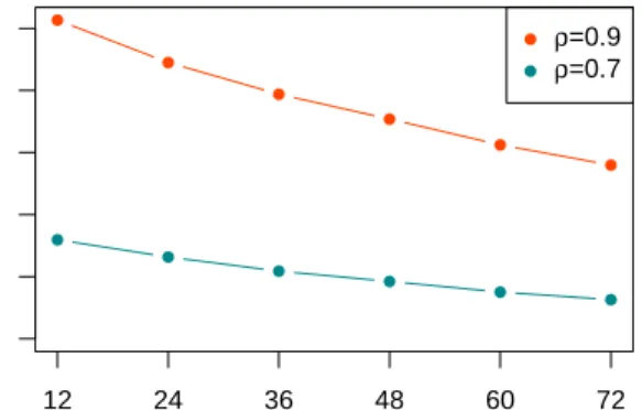
In order to get a first impression about the differences in the clustering results, the resulting numbers of clusters are compared for the different forecast horizons in figure 1. The comparison indicates that the forecast horizon has a substantial influence on spatial dependence of wind power forecast errors. In
● ● ● ● ● ● 0 2000 6000 10000
Forecast horizon (in hours)
Number of clusters ● ● ● ● ● ● ● ● ρ=0.9 ρ=0.7 12 24 36 48 60 72
Figure 1: Number of clusters for different forecast horizons
the moderate correlation scenario (ρ= 0.7), the number of clusters decreases
210
from 3189 clusters for the 12-hour forecasts to 1259 clusters for the 72-hour forecasts. In the high correlation scenario, 10269 clusters are found for the 12-hour forecasts and 5597 clusters for the 72-hour forecasts. Therefore, the
cluster analysis confirms that spatial dependence of wind power forecast errors increases substantially for longer forecast horizons as stated by [18].
215
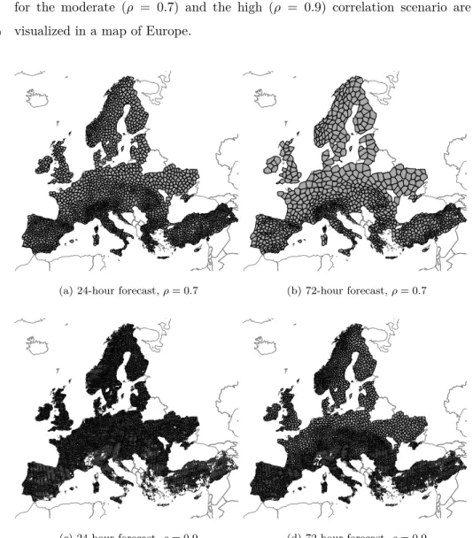
In order to compare different regions of Europe according to their degree of spatial forecast error dependence, we focus on a comparison of the clustering results for the 24- and 72-hour forecast errors. In figure 2, the resulting clusters
for the moderate (ρ = 0.7) and the high (ρ = 0.9) correlation scenario are
visualized in a map of Europe.
220
(a) 24-hour forecast,ρ= 0.7 (b) 72-hour forecast,ρ= 0.7
(c) 24-hour forecast,ρ= 0.9 (d) 72-hour forecast,ρ= 0.9 Figure 2: Clustering of 24- and 72-hour forecast errors
Comparing the two forecast horizons, the clusters for the 72-hour forecast errors are markedly larger than the clusters for the 24-hour forecast errors in all parts of Europe in both correlation scenarios. Besides increasing cluster sizes for longer forecast horizons, figure 2 also reveals striking differences in the cluster sizes in different regions of Europe. In all scenarios, the largest clusters
225
can be found in the low-terrain areas of Northern Europe, Germany, France and Eastern Europe. In these areas, the biggest increase in cluster sizes can be recognized when comparing the 24-hour and 72-hour forecast errors. This fact can be quite interesting since a relatively large amount of wind power plants is installed in these areas. A high correlation of wind power forecast errors of
230
closely located wind power plants can lead to an increased cumulative forecast error for the respective area. The smallest clusters occur in mountain areas like the Alps, the Pyrenees and the Carpathian mountains and in the higher lying areas of Southern Europe and Norway.
With the proposed clustering approach, it is not only possible to explore
235
areas with a relatively high spatial dependence, but also to identify the regions that are characterized by a high number of noise points. These grid cells do not have any spatial neighbor with a correlation higher than the predefined value of
ρ. Areas with a high number of noise points can therefore be regarded as areas
that are characterized by a low spatial correlation of wind power forecast errors.
240
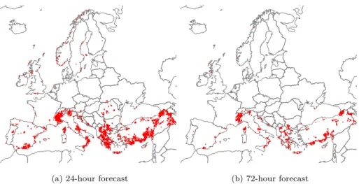
The noise points that are found for the high correlation scenario are visualized in figure 3 for the 24- and 72-hour forecast errors.
For the 24-hour forecast errors, the majority of the noise points can be found in high mountain areas like the French Alps, the Apennines in Italy and the Taurus Mountains in Turkey. In addition, several noise points are located very
245
close to the seaside. The points in coastal areas mostly disappear when regarding the 72-hour forecast horizon. However, a large number of noise points can still be found in the French Alps and in mountain areas of Greece and Turkey, whereas almost no noise points remain in Northern Europe. The number of noise points reduces markedly for longer forecast horizons which results from a
250
● ●● ●● ● ● ● ● ●● ● ● ● ● ● ● ● ● ● ●● ● ●● ●● ● ● ● ●●●●●●●● ● ● ● ● ●● ● ●●●●● ● ● ● ● ● ● ● ●● ● ●●● ● ● ● ●● ● ● ●● ● ● ● ●● ● ● ● ● ●● ● ●●●● ●● ●●● ● ●● ● ●●● ● ●●●●●●● ● ● ●● ●●●●●● ● ● ●●● ● ● ●●●●● ● ● ●●●●●●●●●●●● ●●●●● ● ●● ●●●●● ● ●●●● ●●●●●●●●●● ● ●● ● ●●●●●●●● ●●●●●● ●●●●● ● ● ●●●●●●●●●●●●●●●●●●●● ● ● ●● ● ● ●●●●●●●●●●●●●●● ●●● ● ● ● ● ●● ● ●●●● ● ●●●●●●●●●●●●●● ● ● ● ● ● ●● ●●●●●● ●●●●●●●●● ● ● ●●● ●● ●●●●●●●●●●●●●●● ● ●●● ● ●●●●● ●●●●●● ●●● ●●●●●●●●●●●●● ●●● ●●● ● ●●●●●●●●●● ● ●●●●●●●●●●●● ● ● ●● ●● ●●●●●●●●●●●● ●● ● ● ●●●●●●●●●●● ●●● ● ● ● ● ● ●●●●●●●●● ● ● ●●● ●● ●● ●●● ●● ●● ●●● ● ●● ● ● ● ● ●● ● ● ●●● ● ● ●●● ●● ● ●● ● ● ● ● ● ●●●●●● ● ● ●●● ● ● ● ●●● ● ● ● ●●● ●●●● ● ●●● ● ●● ● ● ● ● ●●● ● ●●●● ●● ● ●●●● ●●● ● ● ● ● ● ● ● ●●●●● ● ● ●●●●●●● ● ●●●●●● ●● ●● ● ●●●● ● ● ●●●●●●●●● ● ●●●●●●● ● ●●● ●●● ● ● ●●●● ● ●●●●●●●● ●●● ● ● ● ●●●● ●●●●●●●●●●●●●● ● ● ● ● ● ● ●●●●●●●●●●●●● ● ● ● ●●● ● ●●●●● ●●●●●● ● ● ●●●● ● ● ●●●● ●●●●● ● ● ●● ● ●● ●●●●●●●● ●● ●● ● ● ● ●● ●● ●●●● ● ● ● ●● ●●●●●●● ● ●●● ● ●●● ●●●●●●●●● ●● ●●● ● ●● ● ● ●●●●●●●●●●●●●● ● ● ●●● ●● ● ● ●●● ●●● ●●●● ●● ●●●●●●●●●●●●●●●● ● ● ● ● ●●●●●●●● ● ●● ● ● ● ●● ● ●●●●●●●●●● ●● ● ● ●●●●●●●●● ●● ●●● ●●●●●●●●● ●● ●●● ● ● ●●●●●● ● ●● ●●●●●●●●●●●●●●●●● ● ● ●●●●●●● ● ●● ●●●●●●●●●●●●●● ●●● ●● ● ●●●●●●●● ● ● ●●●●●●●● ●● ●●● ● ● ● ●●●●●●●●● ● ● ●● ● ●●●●●● ●● ●●● ● ● ● ●●● ●● ●●●●●● ●●●●● ● ●●●●●●● ● ● ●●●● ● ●● ●● ●●● ● ●●●● ●●●●● ●●●● ● ● ●●●● ●●●●●●●● ● ●●●●●●● ●● ● ● ●●●●● ● ●●●●● ●●● ●● ● ●●●● ●●●●●●● ● ●●●●●● ●● ●● ● ●●●● ●●● ● ● ● ● ● ●●●●●●●●●● ●● ●● ●● ●● ●●●●●●●●●●● ● ● ●●●●● ●●●●●●●●● ● ● ● ●●●●●●●● ● ● ●●●●●● ●●●●● ● ●● ●●●●●●●●● ●● ●●●●●●●● ● ●●●●● ●●●●● ●●●●● ●●●●● ●● ● ●●● ●●●●●●●● ●● ● ● ●● ● ●● ●●●● ●●●●●●●●●●● ● ●● ● ●●●●●● ●●●●● ● ●●●●●●●● ●●●●●●●●●● ●● ●● ● ● ● ●● ●●● ●●● ● ● ●●●● ● ●●●●●●●●● ● ●●●●● ●●●●● ● ●● ●● ●● ●● ●●● ● ● ● ●●●●●●● ● ●●●●● ●●●● ● ● ●●● ● ●● ●● ● ● ● ●●●● ● ●●●● ● ● ● ●● ● ● ● ●● ● ● ●●●● ● ● ● ● ● ●● ●●● ●● ● ● ●● ●● ● ● ● ● ● ●●●●●●● ●● ●●●●● ● ●● ●● ● ●● ●●●●●● ●●● ● ● ●●●●●●●●● ● ●●●●● ●● ●●● ● ●●● ●● ● ●●● ● ●● ●●● ●●● ●●●●●●●●●● ●●●●●● ● ●● ●●●●● ●●●●●● ●● ●●●● ●●●● ● ● ● ●●● ●●●●● ●●●● ●●●●●●● ●●●●●● ●●●●● ●●●●●●●●●●●●● ●●●● ● ●●●●●●●●●●● ●●●●● ●●●● ●●●●●●●●●●●● ●● ●● ●●●● ● ●● ●●●● ●●●●●●●●●●●●●●● ● ●●●●● ●●●● ●●● ●●●●● ● ●●● ●●●●●●●●●● ●● ●● ●●●●● ●●●●●●●●●●●●●●●●●●●●●● ●●●● ●●●● ● ● ●●●● ● ● ●●●● ● ●● ● ●●●●●●●● ●●●●●●●●●●●●●●●●●●●●● ●●●●●● ● ● ●● ● ● ● ●●● ● ●●●●● ● ● ● ●●●●●●●●●●●●●●● ●●● ● ● ●●●●● ● ●● ●● ●●● ●● ●●●● ●● ● ●●●●●●●●●● ● ● ●●●●●●●●●● ●●●●●●●● ●● ● ●● ●● ●●● ●●●●●●●● ●●●●●●● ● ●●●●●●●●● ●●●●●●●● ● ●● ●●●●●●●●●●●●● ●●●●●● ●●●●●●●● ● ● ●● ●●●●●●●●● ● ●●●●● ●● ●●●●●●●●●●●●●●●●●● ●●●●● ● ●●●●●● ● ● ●●● ● ●●●●●●●●●●●●●● ● ●●●●●●●●●●●●●●● ●●●● ●●●● ● ● ●●●●●●●●●●●● ●●●●●●●●●●●●●●●●●● ●●● ● ●●●●●●●●● ● ●●●●●● ●●●●●● ●●●● ● ●● ●●●● ●●●●●●●●● ● ●● ●●●● ●● ● ● ● ●● ●●●●●●● ●●● ●●●●●●●●● ●● ●● ●●
(a) 24-hour forecast
● ● ● ● ●● ● ● ●● ●●●●●●●●●● ● ● ● ●●● ● ●●●●●● ●● ●●●● ●●●● ● ●●●●●●●● ● ●●●●●●●●●●●●● ● ● ●●●●●●●●●●●●●●● ● ●●●●● ●●● ●●●● ●● ●●●● ●●● ●●●● ●● ●●● ● ●●● ●●● ● ● ●●●●●●●●●● ●● ● ●●●●●●● ●●● ● ● ●●● ●●● ● ●● ● ● ● ● ●● ● ● ● ● ● ●●●● ● ● ● ●●● ● ● ● ●●● ●●●● ● ● ● ● ● ●●● ● ●●●●● ● ● ● ●●● ●● ●●● ●●●●●● ●●●● ● ●●●●● ●●●● ● ● ● ● ● ● ● ● ●● ●● ● ●●● ●●●●●● ● ● ●●● ●●●●●●●●●●●● ● ●● ● ●●●●●●●●●●●● ● ● ● ●●● ●● ●●●●●●●● ●●● ●● ●●●●●●●●● ● ● ●●●●●●●●● ●● ● ●●●●● ●● ● ●● ● ● ●●● ● ● ● ● ●●● ●●●● ●●●●● ●●● ● ● ● ● ●●● ●● ●● ●●●● ● ● ●● ● ● ● ●● ●●● ● ●● ● ● ● ●●●●●●● ●● ●● ●● ●●●●●●● ●● ● ●● ●● ● ● ●● ●● ● ● ● ● ● ●● ● ●●● ● ●● ● ● ● ● ●● ●●●●● ● ● ● ● ● ● ●●●●● ●●● ● ● ● ● ● ● ● ● ● ● ● ●●●● ●● ● ● ● ● ● ● ● ● ●●● ●● ●● ● ● ●● ●● ● ●●●● ● ● ●● ●● ● ●● ●●●●●●●●● ●●● ●● ●● ● ● ●●●●●●●●●●●● ●●●● ●● ● ● ● ●●●●●● ● ● ● ● ●●●●● ●● ●● ●●● ●● ●●● ● ●● ● ●● ●●●● ●● ●● ●● ● ●●● ●● ●● ●● ●● ● ●● ● ●●●●●● ● ● ● ●●● ● ●● ●●● ●●●●● ●●● ●●●●● ● ● ●●●●●●●●●● ●●●●● ●● ●●●●● ● ● ●●●●●● ● ●●●●●●●●●●● ●●●● ● ●● ●●●● ●●●●● ● ● ●● ● ●● ●● ●● ●●● ●●● ●● (b) 72-hour forecast
Figure 3: Noise points found with the 24- and 72-hour forecast error clustering (ρ= 0.9)
4. Extension: Combination of Clustering Results from Multiple Sub-regions
The application in the previous section has demonstrated that the pro-posed algorithm can provide a highly efficient way to cluster big spatio-temporal
255
datasets. Nevertheless, memory limitations can still be an issue when the
num-ber of spatial pointsN increases. Regarding the example of wind power forecast
errors, this problem could occur, for instance, when other large countries like Russia shall also be considered in the analysis. In addition, the resolution of meteorological forecasts steadily increases in order to achieve a higher
forecast-260
ing accuracy. Exemplarily, the European Centre for Medium-Range Weather Forecasts (ECMWF) reduced the horizontal grid spacing for the deterministic forecasts from 16 km to 9 km in March 2016 [23]. In order to prevent issues that may occur due to memory limitations, an extension of the clustering strategy is presented in this section. The extension builds on the idea that the full study
265
region can be divided into multiple subregions for which a separate clustering can be conducted. As far distant points are generally not strongly related to each other, clusters located far away from another subregion should remain
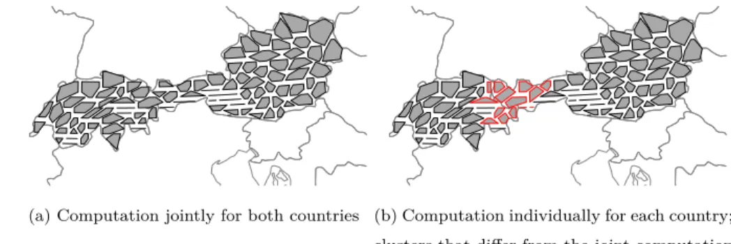
un-affected from splitting the study region. As an example, we conduct a clustering of 12-hour wind power forecast errors for spatial points located in Austria and
270
Switzerland (for ρ= 0.7). The clustering is performed once for both countries
jointly and once for the two countries individually. The resulting clusters for both approaches are visualized in figure 4. Clusters from the individual clus-tering that are different compared to the joint clusclus-tering are highlighted in red. The comparison reveals that the clustering structure differs only in the region
275
close to the border of the two countries.
(a) Computation jointly for both countries (b) Computation individually for each country; clusters that differ from the joint computation are highlighted in red
Figure 4: 12-hour forecast error clustering of spatial points located in Austria and Switzerland (ρ= 0.7)
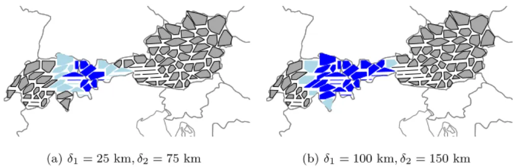
In order to combine the clustering results of multiple subregions, hence only those spatial points need to be reprocessed that belong to a cluster close to the border to another subregion. By defining inner edge clusters (clusters with
at least one spatial point located within a distance δ1 to the closest point of
280
another subregion) and outer edge clusters (clusters not belonging to the inner
edge clusters and with at least one spatial point located within a distanceδ2to
the closest point of another subregion), the spatial points in the border regions can be determined for which an additional clustering needs to be conducted. While the points located in the outer edge clusters keep their cluster labels
285
clustering for the entire study region), the cluster labels of the spatial points belonging to the inner edge clusters are removed. For the example of clustering 12-hour wind power forecast errors in Austria and Switzerland (individual com-putation), the respective inner and outer edge clusters are visualized for two
290
different choices ofδ1 andδ2in figure 5. A new dataset is created that contains
the time series and the cluster labels of the spatial points belonging to one of the inner or one of the outer edge clusters and an additional clustering is performed for these points.
(a)δ1= 25 km, δ2= 75 km (b)δ1= 100 km, δ2= 150 km Figure 5: Edge clusters for the 12-hour forecast error clustering (ρ= 0.7) in Austria and Switzerland (individual computation) for two different choices of the parametersδ1 and δ2. Inner edge clusters are highlighted in dark blue and outer edge clusters in light blue.
In order to present the idea of the clustering extension in detail, we
as-295
sume that the full dataset D can be divided into R subdatasets (subregions)
D(1), . . . , D(R). The number of time steps T is required to be equal in each
subdatasetD(r)(r= 1, . . . , R), whereas the number of spatial pointsN(r) may
differ. For each subdataset, a separate clustering is initially performed with the
algorithm proposed in section 2. This results in a number ofc(r)clusters for the
300
respective subdatasetD(r). Before the clusters from the different subdatasets
can be combined, their cluster labels need to be changed in order to avoid clus-ters with the same label from different subdatasets. Therefore, the clusclus-ters from
the first subdatasetD(1)keep their cluster labelsC1, . . . , Cc(1) whereas the
clus-ters from the second subdatasetD(2) receive the labels Cc(1)+1, . . . , Cc(1)+c(2),
the clusters from D(3) the labels C
c(1)+c(2)+1, . . . , Cc(1)+c(2)+c(3) and so forth.
Subsequently, the following steps can be performed to receive a clustering solu-tion for the entire study region:
Step 1. Determine the set of inner edge points
s(innerr) ={s∈D(r)| min
t∈{D(1),...,D(R)}\D(r)
dist(s, t)≤δ1}
for each subdatasetD(1), . . . , D(R). Save the entire list of inner edge points
in a set sinner = ∪r∈{1,...,R}s(
r)
inner and the corresponding cluster labels
(uniquely) in a set Cinner.
Step 2. Determine the set of outer edge points
s(outerr) ={s∈D(r)| min
t∈{D(1),...,D(R)}\D(r)δ1<dist(s, t)≤δ2}
for each subdatasetD(1), . . . , D(R). Save the entire list of outer edge points
in a set souter = ∪r∈{1,...,R}s
(r)
outer and the corresponding cluster labels
(uniquely) in a setCouter (without clusters that already belong toCinner).
Step 3. Create a new dataset Dedge with the spatial points that belong
to a cluster listed in Cinner or Couter and the points in sinner that were
marked as noise by the clustering algorithm.
Step 4. Set all cluster labels of the spatial points in Dedgethat belong to
a cluster listed inCinner to zero and apply the clustering strategy proposed
in section 2 on the new dataset. This leads to new clusters that are marked by new cluster labels.
Step 5. Combine the clustering results for the border area from step 4 with the results for the remaining spatial points. This leads to a final clustering solution.
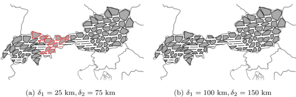
In order to test the proposed approach, we consider again the example of clustering 12-hour wind power forecast errors in Austria and Switzerland.
The clustering results that were obtained individually for each country are now combined with the clustering extension described above. The combina-tion of the clustering results is performed once with comparatively small values
ofδ1= 25 km andδ2= 75 km and once with higher values ofδ1= 100 km and
δ2= 150 km. The results are visualized in figure 6.
315
(a)δ1= 25 km, δ2= 75 km (b)δ1= 100 km, δ2= 150 km Figure 6: 12-hour forecast error clustering of spatial points located in Austria and Switzerland (ρ= 0.7). The clustering was conducted separately for each country and the clusters were combined subsequently with the proposed clustering extension. Clusters that differ from the joint computation are highlighted in red.
Regarding the clusters that are obtained for small values of the parameters
δ1 andδ2, differences compared to the joint computation are still prominent in
the area close to the border. However, when the values of the parameters are increased, the clustering results tend to be more similar to those obtained with
the joint computation. For values of δ1 = 100 km and δ2 = 150 km, it turns
320
out that the clustering structure already equals the one observed with the joint computation. In general, both computation methods are able to highlight the same regions in which higher or lower spatial correlations are present and are
thus able to capture the dependence structure equally well. The distances δ1
andδ2need to be predefined related to the degree of correlationρthat is chosen
325
for the clustering process. As a higher value ofρleads to smaller clusters and
therefore to a more similar clustering structure close to the borders, generally
This makes the proposed method highly efficient and therefore attractive for many practitioners who intend to preprocess and reduce big spatio-temporal
330
datasets. With the extension, the clustering process can easily be parallelized which leads to major improvements in performance.
5. Discussion: Comparison with other Clustering Algorithms
In order to distinctly point out the advantages of CorClustST and to dis-cuss possible disadvantages, this section addresses differences and similarities
335
between the proposed method and the most popular clustering algorithms that are currently employed for spatio-temporal data. Table 1 compares the pro-posed algorithm with several clustering methods regarding important features like complexity, memory requirements, parallelization and interpretability.
For big spatio-temporal datasets, the most popular clustering algorithms
340
like thek-means algorithm or hierarchical clustering methods are generally less
efficient than specifically designed spatio-temporal clustering methods like
ST-DBSCAN or ST-OPTICS. Regarding thek-means algorithm, it is particularly
necessary to perform the clustering for different values ofkwith heuristic criteria
like the elbow criterion [26] to find an optimal clustering solution. This can
345
be a major drawback in case of extremely large datasets. A hybrid clustering framework, however, could serve as an efficient alternative: Schyska et al. (2017)
[27] propose a combination of thek-means algorithm and hierarchical clustering
for the reference site selection of wind farms. They first cluster the locations into
geographical clusters with the k-means algorithm and select the site with the
350
highest wind power capacity for each cluster. Subsequently, pairwise (temporal) correlations between the selected sites are computed and a hierarchical clustering is applied to find the final reference sites. However, this approach is only valid when meaningful additional information (such as installed wind power capacity) is available.
Table 1: Comparison of CorClustST with existing algorithms regarding complexity, paral-lelization and interpretability for spatio-temporal data.
Algorithm Complexity, Parallelization Computation, Interpretability for Spatio-Temporal Datasets
k-means
• Complexity: O(N·T ·k·i), withkthe number of clusters,
T the number of time points andithe number of iterations [24]
• Large-scale parallelization not directly possible, requires computation of a distance matrix with N(N−2 1) entries
Disadvantages:
• Not specifically designed for spatio-temporal data
• The number of clusters has to be predefined with heuristic criteria
• All observations have to be assigned to a cluster
• Comparison of clustering results for different scenarios can be difficult Advantage:
• Meaningful cluster centers are provided for the purpose of data reduction and for analyzing cluster interconnections
Hierarchical Clustering (Complete Linkage) • Complexity:O(N2·logN) [25] • Large-scale parallelization not directly possible, requires computation of a distance matrix with N(N−2 1) entries
Disadvantages:
• Not specifically designed for spatio-temporal data
• Cluster centers are not directly provided
• All observations have to be assigned to a cluster
• Comparison of clustering results for different scenarios can be difficult Advantage:
• The number of clusters does not have to be predefined (however a suitable stopping criterion needs to be chosen)
ST-DBSCAN, ST-OPTICS
• Complexity: O(N·logN) [11]
• Large-scale parallelization dif-ficult, could be achieved with a similar technique as pro-posed in section 4
Disadvantages:
• Cluster centers are not directly provided
• Comparison of clustering results for different scenarios can be difficult Advantages:
• Specifically designed for spatio-temporal data (high efficiency)
• The number of clusters does not have to be predefined
• Not all observations have to be assigned to a cluster, unusual observations are declared as noise points
CorClustST
• Complexity: O(N·logN) for small values of , O(N2) for
→ ∞
• Large-scale parallelization possible with the extension proposed in section 4
Disadvantages:
• The clustering solution is not optimized regarding a specific quality criterion
• Higher complexity than ST-DBSCAN and ST-OPTICS for large values of
Advantages:
• Specifically designed for spatio-temporal data (high efficiency)
• The number of clusters does not have to be predefined
• Not all observations have to be assigned to a cluster, unusual observations are declared as noise points
• Meaningful cluster centers are provided for the purpose of data reduction and for analyzing cluster interconnections
• Clusters for different scenarios and different spatial regions can be compared easily as cluster sizes depend directly on the degree of spatial correlation
CorClustST provides an efficient way to cluster all spatial points directly without the requirement of additional information: The proposed algorithm has a comparatively low complexity and requires only little memory space, especially
when a small value is chosen for the parameterwhich controls the number of
spatial neighbors considered for the clustering. For small values of, less spatial
360
neighbors are taken into account and therefore in total less pairs of spatial points need to be processed. The complexity of CorClustST is then comparable to the complexity of ST-DBSCAN and ST-OPTICS. Contrary to these algorithms, CorClustST computes empirical correlations between predetermined pairs of spatial points before assigning them into clusters. This avoids using a stack that
365
leads to multiple computations for the same pairs of points. By considering only relevant pairs of spatial points and by computing their correlations in advance, the clustering process is more easy to parallelize than the stacked versions of ST-DBSCAN and ST-OPTICS. Furthermore, the extension proposed in section 4 allows for a large-scale parallel implementation that can markedly improve
370
computation times. Existing spatio-temporal clustering methods do currently not allow for such a large-scale parallelization.
Regarding the interpretability of the results, the proposed clustering
strat-egy combines different advantages of existing clustering techniques like the k
-means algorithm and ST-DBSCAN: One very helpful feature of the k-means
375
algorithm is that it provides cluster centers that can be utilized for the purpose of data reduction and for further analysis of cluster interconnections. However,
the number of clusterskneeds to be predetermined in advance which is a
ma-jor drawback for big spatio-temporal datasets. The spatio-temporal clustering algorithms ST-DBSCAN and ST-OPTICS do not require a predefined
num-380
ber of clusters but they do, however, not provide meaningful cluster centers. These drawbacks are addressed by CorClustST. Here, the number of clusters does not have to be predefined in advance and meaningful cluster centers are provided which correspond to those spatial points with the highest number of
spatio-temporal neighbors in certain regions. If a high value ofρ is chosen for
385
intuitively by focusing on the cluster centers that are characteristic for the
re-spective regions. Another advantage of CorClustST compared to thek-means
algorithm or hierarchical clustering methods is that it shares the possibility of density-based clustering algorithms to determine noise points.
390
For several applications such as the example of wind power forecast errors, it may be required that the applied clustering technique directly allows to com-pare the strength of possible spatial dependencies for different scenarios (e.g. different forecast horizons) and for different regions. In this sense, CorClustST clearly separates from the other discussed clustering strategies. The goal of
395
common clustering algorithms mainly is to find an optimal clustering solution by minimizing the distances (defined by metrics like the Euclidean distance) between observations within a cluster and maximizing the distances between observations that belong to different clusters. This requires to optimize control
parameters such as the number of clusters k for thek-means algorithm [4] or
400
the parametersM inP ts, Eps1,Eps2 and ∆for ST-DBSCAN [10] in advance
via heuristic criteria. As these parameters need to be adjusted to find optimal clustering solutions for different scenarios, the clustering results are difficult to compare because different control parameters lead to a completely different interpretation of the resulting clusters. Since CorClustST uses empirical
cor-405
relations to determine the clusters, the algorithm allows to compare different
clustering results by fixing the value ofρ(the desired degree of spatial
correla-tion which is easy to interpret) for all scenarios.
Contrary to the other algorithms, the main goal of CorClustST is therefore not to find an optimal clustering solution regarding the (dis)similarity of the
410
objects, but rather to provide an efficient descriptive tool to compare the degree of spatial dependence for different scenarios and different spatial regions. As CorClustST does not compete with the other discussed algorithms in this sense, we refrain from comparing the algorithms regarding computation times and cluster validity. Although CorClustST was not mainly designed for this purpose,
415
the algorithm can still be a helpful tool when an optimal clustering solution shall be found: If the number of spatial points in the dataset is too large to perform a
clustering efficiently with traditional clustering methods, CorClustST can first be applied with rather high correlation thresholds to reduce the dataset. The reduced dataset, which should consist of the cluster centers and the noise points
420
that do not belong to a cluster, can subsequently be processed with the desired clustering technique in order to find an optimal clustering solution.
6. Conclusion and Future Work
Spatio-temporal clustering is a popular way to identify patterns in mas-sive spatio-temporal datasets. As currently employed clustering methods still
425
have some drawbacks regarding the comparability and the interpretability of the results, an alternative strategy for clustering big spatio-temporal datasets has been proposed in this paper. CorClustST clusters the spatial points in a dataset based on spatial correlations over time and makes it better possible to compare clustering results for varying periods of time and multiple underlying
430
variables than with existing algorithms. In a test case, the algorithm success-fully identified increasing spatial correlations of wind power forecast errors for longer forecast horizons and highlighted those regions of Europe in which spatial dependence is mostly prominent. It was also shown that the clustering method can be easily extended in such way that it allows for an efficient large-scale
435
parallelization while preserving the essential clustering structure. With the pro-posed approach, a clustering of big spatio-temporal datasets can be performed even on systems with only little memory capacity. Other than currently em-ployed methods, the clustering strategy additionally provides meaningful cluster centers which makes it especially valuable for the purposes of preprocessing and
440
data reduction.
For future research, the insights gained with the clustering of wind power forecast errors in chapter 3 increase the need for analyzing spatial dependence of wind power forecast errors in more detail. Spatio-temporal copulas [28], for instance, could be used to model the full dependence structure of wind power
445
fore-cast horizons also lead to increasing tail dependencies (i.e. whether extremely large forecast errors tend to occur jointly at closely located grid cells). By using calibrated meteorological ensemble forecasts [29, 30, 31], it could furthermore be possible to better assess the risks that occur due to spatial dependence of wind
450
power forecasts for long forecast horizons. The information from the ensemble forecasts could, for instance, be used for grid security calculations and could also help to improve probabilistic electricity price forecasts [32, 33].
Acknowledgements
We wish to thank Uwe Ligges from TU Dortmund University for helpful
455
comments and suggestions. During his research stay at the Center for Wind
Energy Research (ForWind) in Oldenburg, Germany, Marc H¨usch has received
funding from the Alumni-Verein Dortmunder Statistikerinnen und Statistiker.
Bruno U. Schyska has received funding from the European Union’s Seventh Programme for research, technological development and demonstration under
460
grant agreement No. 609795 (IRPWind). Lueder von Bremen has received funding from the ministry of science and culture of Lower Saxony, Germany in the project ventus efficiens (No. ZN3024).
References
[1] L. Kaufman, P. J. Rousseeuw, Finding Groups in Data: An Introduction
465
to Cluster Analysis, Wiley Series in Probability and Statistics, Wiley, 2008. [2] B. Everitt, S. Landau, M. Leese, D. Stahl, Cluster Analysis, Wiley Series
in Probability and Statistics, Wiley, 2011.
[3] K. Ericson, S. Pallickara, On the performance of high dimensional data clus-tering and classification algorithms, Future Generation Computer Systems
470
[4] J. A. Hartigan, M. A. Wong, Algorithm AS 136: A K-Means Cluster-ing Algorithm, Journal of the Royal Statistical Society. Series C (Applied Statistics) 28 (1) (1979) 100–108.
[5] R. Sibson, SLINK: an optimally efficient algorithm for the single-link cluster
475
method, The Computer Journal 16 (1) (1973) 30–34.
[6] D. Defays, An efficient algorithm for a complete link method, The Com-puter Journal 20 (4) (1977) 364–366.
[7] J. H. Ward, Hierarchical grouping to optimize an objective function, Jour-nal of the American Statistical Association 58 (301) (1963) 236–244.
480
[8] S. Kisilevich, F. Mansmann, M. Nanni, S. Rinzivillo, Spatio-temporal clus-tering, in: O. Maimon, L. Rokach (Eds.), Data Mining and Knowledge Discovery Handbook, Springer US, 2010, Ch. 44, pp. 855–874.
[9] M. Ester, H.-P. Kriegel, J. Sander, X. Xu, A density-based algorithm for discovering clusters in large spatial databases with noise, in: KDD-96
Pro-485
ceedings, AAAI Press, 1996, pp. 226–231.
[10] D. Birant, A. Kut, ST-DBSCAN: An algorithm for clustering spatial– temporal data, Data & Knowledge Engineering 60 (1) (2007) 208–221. [11] K. Agrawal, S. Garg, S. Sharma, P. Patel, Development and validation of
OPTICS based spatio-temporal clustering technique, Information Sciences
490
369 (2016) 388–401.
[12] M. Ankerst, M. M. Breunig, H.-P. Kriegel, J. Sander, OPTICS: Ordering Points to Identify the Clustering Structure, in: Proceedings of the 1999 ACM SIGMOD International Conference on Management of Data, SIG-MOD ’99, ACM, 1999, pp. 49–60.
495
[13] K. Pearson, Note on regression and inheritance in the case of two parents, Proceedings of the Royal Society of London Series I 58 (1895) 240–242.
[14] C. Spearman, The proof and measurement of association between two things, The American Journal of Psychology 15 (1) (1904) 72–101. [15] M. G. Kendall, A new measure of rank correlation, Biometrika 30 (1-2)
500
(1938) 81.
[16] R. Taylor, Interpretation of the correlation coefficient: A basic review, Journal of Diagnostic Medical Sonography 6 (1) (1990) 35–39.
[17] M. Lange, On the uncertainty of wind power predictions - Analysis of the forecast accuracy and statistical distribution of errors, Journal of Solar
505
Energy Engineering 127 (2) (2005) 177–184.
[18] U. Focken, M. Lange, K. M¨onnich, H.-P. Waldl, H. G. Beyer, A. Luig,
Short-term prediction of the aggregated power output of wind farms - a sta-tistical analysis of the reduction of the prediction error by spatial smoothing effects, Journal of Wind Engineering and Industrial Aerodynamics 90 (3)
510
(2002) 231–246.
[19] J. Tastu, P. Pinson, E. Kotwa, H. Madsen, H. A. Nielsen, Spatio-temporal analysis and modeling of short-term wind power forecast errors, Wind En-ergy 14 (1) (2011) 43–60.
[20] ECMWF, Medium-range forecasts, 2016, published online: http:
515
//www.ecmwf.int/en/forecasts/documentation-and-support/ medium-range-forecasts(Last visited: June 01, 2017).
[21] S. Sp¨ath, L. von Bremen, C. Junk, D. Heinemann, Time-consistent
calibra-tion of short-term regional wind power ensemble forecasts, Meteorologische Zeitschrift 24 (4) (2015) 381–392.
520
[22] EWEA, Wind in power: 2015 European statistics, 2016,
pub-lished online: https://windeurope.org/wp-content/uploads/files/
about-wind/statistics/EWEA-Annual-Statistics-2015.pdf(Last vis-ited: June 01, 2017).
[23] ECMWF, New forecast model cycle brings
highest-525
ever resolution, 2016, published online: http://
www.ecmwf.int/en/about/media-centre/news/2016/
new-forecast-model-cycle-brings-highest-ever-resolution (Last visited: June 01, 2017).
[24] C. Aggarwal, C. Reddy, Data Clustering: Algorithms and Applications,
530
Chapman & Hall/CRC Data Mining and Knowledge Discovery Series, Tay-lor & Francis, 2013.
[25] Y.-J. Oyang, C.-Y. Chen, T.-W. Yang, A study on the hierarchical data clustering algorithm based on gravity theory, in: Proceedings of the 5th Eu-ropean Conference on Principles of Data Mining and Knowledge Discovery,
535
PKDD ’01, Springer Berlin Heidelberg, 2001, pp. 350–361.
[26] R. L. Thorndike, Who belongs in the family?, Psychometrika 18 (4) (1953) 267–276.
[27] B. U. Schyska, A. Couto, L. von Bremen, A. Estanqueiro, D. Heinemann, Weather dependent estimation of continent-wide wind power generation
540
based on spatio-temporal clustering, Advances in Science and Research 14 (2017) 131–138.
[28] B. Gr¨aler, Developing spatio-temporal copulas, Ph.D. thesis, Westf¨alische
Wilhelms-Universit¨at M¨unster (2014).
[29] T. Gneiting, F. Balabdaoui, A. E. Raftery, Probabilistic forecasts,
cali-545
bration and sharpness, Journal of the Royal Statistical Society: Series B (Statistical Methodology) 69 (2) (2007) 243–268.
[30] T. Gneiting, A. E. Raftery, A. H. Westveld III, T. Goldman, Calibrated probabilistic forecasting using ensemble model output statistics and min-imum CRPS estimation, Monthly Weather Review 133 (5) (2005) 1098–
550
[31] A. E. Raftery, T. Gneiting, F. Balabdaoui, M. Polakowski, Using Bayesian model averaging to calibrate forecast ensembles, Monthly Weather Review 133 (5) (2005) 1155–1174.
[32] T. J´onsson, P. Pinson, H. A. Nielsen, H. Madsen, T. S. Nielsen, Forecasting
555
electricity spot prices accounting for wind power predictions, IEEE Trans-actions on Sustainable Energy 4 (1) (2013) 210–218.
[33] T. J´onsson, P. Pinson, H. Madsen, H. A. Nielsen, Predictive densities for
day-ahead electricity prices using time-adaptive quantile regression, Ener-gies 7 (9) (2014) 5523–5547.
Marc H¨usch received his B.Sc. and his M.Sc. in Statistics from TU Dortmund University, Germany. During his studies, he was a visiting research intern at the National Renewable Energy Laboratory (NREL) in Golden (CO), USA and at the Center for
565
Wind Energy Research (ForWind) in Oldenburg, Germany. He is currently pursuing a Ph.D. in Statistics at TU Dortmund University, where he is working on problems in the fields of data mining and spatial statistics.
Bruno U. Schyska received his B.Sc. in Physics from
Uni-570
versity Bremen, Germany, and his M.Sc. in Meteorology from
Freie Universit¨at Berlin, Germany. He is currently working as a
research assistant in the energy meteorology group at University of Oldenburg’s ForWind Center for Wind Energy Research in Oldenburg, Germany.
575
Lueder von Bremen received his Diploma in Meteorology at the University of Kiel, Germany in 1997 and his Ph.D. in 2001. From 2001-2005 he worked at the European Centre for Medium-Range Weather Forecasts and continued his career at ForWind,
580
Center for Wind Energy Research at the University of Olden-burg, Germany. He has more than 15 years of experience in wind energy and Numerical Weather Prediction. Dr. von Bremen leads the team on “Energy Weather Forecasting and Analysis” and is interested in the design and manage-ment of the future European power supply system based on renewable energies.