Nijmegen
The following full text is a publisher's version.
For additional information about this publication click this link.
http://hdl.handle.net/2066/105783
Please be advised that this information was generated on 2017-12-06 and may be subject to
change.
Methods and Applications
SIKS Dissertation Series No. 2013-09
The research reported in this thesis has been carried out under the auspices of SIKS, the Dutch Research School for Information and Knowledge Systems.
Computational Methods
and
Applications
Proefschrift
ter verkrijging van de graad van doctor aan de Radboud Universiteit Nijmegen
op gezag van de rector magnificus prof. mr. S.C.J.J. Kortmann, volgens besluit van het college van decanen
in het openbaar te verdedigen op 9 april 2013 om 15:30 uur precies
door
Fabio Gori
geboren op 5 november 1979 te Pistoia, Itali¨e
Prof. dr. T.M. Heskes Prof. dr. ir. M.S.M. Jetten
Copromotor:
Dr. E. Marchiori
Manuscriptcommissie: Prof. dr. N.M. van Dam
Prof. dr. D. Huson - University of T¨ubingen, DE Dr. S.A.F.T. van Hijum
This thesis on microbial populations was possible thanks to the support of a relatively large population of humans. In the first place, I would like to express my deepest gratitude to my daily supervisor Elena and my promotores Mike and Tom. Elena was able to introduce me effectively and quickly in the world of scientific research, and supported me with patience in these four years. Her suggestions on science and on the directions to take were very precious; I hope I gave her good laughs in return. I want to thank Mike for having accepted me as a PhD student of him despite I did not have a background in biology, for his contribution to this work, and for his capacity of explaining the biology to me in a very comprehensible way. Tom had always the door open to me when I needed his advices, especially on the decisions to make; he helped me to put things in perspective and be more optimistic.
I am also thankful to all my other co-authors and the people I worked with: Gianluigi, Huub, Sacha, Dimitris, Boran, Susannah, and Victor. I thank them for their patience to cope with my bad Tuscan temperament, their help, and their close inspection of my writings. Moreover, I would like to thank Prof. dr. van Dam and Prof. dr. Huson for being part of my thesis committee.
I am grateful to my colleagues of the Machine Learning group for our fruitful discussions and for the nice time we spent together: Ali, Pavol, Botond, Tom, Saiden, Adriana, Wout, Max, Daniel, Tjeerd, Joris, Perry, Marcel, Saskia, Maya, Suzan. A special thank to Twan, for having helped me with the Dutch translations of the summary of the present thesis, and for the interest he showed in my questions, not only scientific, at the office. I also want to thank the other colleagues of Intelligent Systems section and ICIS for the scientifically-entertaining lunches and chats at the coffee machines: Olha, Carst, Alexandra, Kasper, Josef, Giulio, Helle, Robbert, Cezary, James, Janos, Herman, Henk, Christiaan, Wessel, Freek, Ilona, Wenyun, Faranak, Fides, Alejandro, Lukasz, Jasper, Flavio, Miguel. Thanks to Nicole and Simone for their kindness and their help, and to Stijn for our open conversations.
Depart-Francisca, Wouter, Ming, Naomi, Daan, Sarah, Harry, Arjan, Jan, Xristina, Olivia, Adam, Jennifer, Maartje, Nardy, Baoli, Marjan, Laura, and Theo.
Tango played an important role in the last three years of my PhD, helping me to have a life outside my research, to increase my self-confidence and to discover a new path to perfection. This was possible thanks to the tango part-ners I had in these years: Karolina, Anna, Georgeta, Wilma, Karola, Svetlana. In particular, I would like to thank Cheng hua for having showed me a new path to tango and having supported me in some troubled times.
In this four years I had the possibility to share the house with amazing people from all around Europe, that helped me significantly in my social life; thanks to Vicen¸c, Christian, Hilje, and Christina. I am particularly grateful to the previous and current tenants of “Casa Italia”, I have always felt at home in that house: Davide, Maresa, Paola, Melina. Thanks also to my friend and neighbour Nina, I hope she liked my bread.
I would like to show my gratitude to all the other Italians of Nijmegen for the nice conversations we had, like Michele G, Francesco, Alberto, Manuela, Ruggero, and all the other Italians I met in these years. I thank also all the lovely guys I met during the last year, like Gianluigi, Roberta, Valentina, Giovanni, Cristina, and, last but not least, the ones who elected me as their major: Michele V, Davide, and Francesca.
As I moved to Netherlands, I luckily got in touch with a splendid group of expats (with some infiltrated Dutches) that instantly welcomed me. Discov-ering other cultures through their friendship was an amazing experience that changed my life: Shankar&Helene and their lovely barbecues, Jordan&Kim, Dennis, Daniela, Ga¨el, Ljupcho&Lilia, Marta, Mariam&Vanja, Anastasia, Tamara, Bart, Alison, Ramona, Doina, Maartje, Thaban, Denise, Mohammad, Natalia, Daniel, Andr´e, Rita, Alexis, Fred, Lies, and Alicja.
My impact to Dutch culture was made soft and pleasant by Hein, a very special friend of mine. We had very funny and enjoyable dinners at the Refter, spiced with conversations about Italy, the Netherlands, and the clich´e topics of Italian gentlemen’s chats. Not to mention that he showed me some artistic Dutch gems that I would not have seen without him.
Finally I want to thank my parents, my aunties, my brother, and his new family, for their support through all my studies. Grazie, perch´e senza di voi non sarei potuto arrivare fin qui.
Acknowledgements v
1 Introduction 1
2 Similarity-based binning at protein level 7
2.1 Introduction . . . 7 2.2 Methods . . . 9 2.2.1 LWproxy . . . 10 2.2.2 GWproxy . . . 13 2.3 Experiments . . . 14 2.3.1 Evaluation . . . 15
2.3.2 Results: fixed value ofα= 0.01 and varying K values . 17 2.3.3 Results: fixed value ofK = 50 and varyingα values. . . 18
2.4 Conclusions and Future Work . . . 21
3 Similarity-based binning at multiple taxonomic ranks 23 3.1 Introduction . . . 23
3.2 Methods . . . 26
3.2.1 Read Assignment at Multiple Taxonomic Ranks . . . . 27
3.3 Experiments . . . 30
3.3.1 Data . . . 30
3.3.2 Aligning reads with protein sequences . . . 31
3.4 Results . . . 31
3.4.1 Results on simulated datasets . . . 32
3.4.2 Results on real-life datasets . . . 38
3.5 Discussion . . . 40
4 Genomic signatures in metagenomics 43 4.1 Background . . . 43
4.2 Methods . . . 46
4.2.2 Data acquisition and preprocessing . . . 49
4.2.3 Computing signatures values . . . 50
4.2.4 Evaluating the effectiveness of signatures . . . 51
4.3 Results and Discussion . . . 53
4.4 Conclusions . . . 57
5 The metagenomic basis of anammox metabolism inCandidatus ‘Brocadia fulgida’ 61 5.1 Introduction . . . 61
5.2 B. fulgida metagenome . . . 62
5.2.1 Inorganic nitrogen transport proteins ofB. fulgida . . . 63
5.2.2 Genes in nitrogen catabolism ofB. fulgida . . . 65
5.3 Conclusions . . . 69
6 Combining sequencing technologies for the retrieval of Candi-datus ‘Brocadia fulgida’ 71 6.1 Background . . . 71
6.2 Results and Discussion . . . 73
6.2.1 Taxonomic annotation and GC-content analysis of anno-tated reads . . . 73
6.2.2 Comparative analysis of recoveredB. fulgida ORFs . . . 74
6.2.3 Comparative analysis of ORF location distribution and functional content . . . 76
6.3 Conclusions . . . 76
6.4 Methods . . . 77
6.4.1 Datasets . . . 77
6.4.2 Annotation Method . . . 78
6.4.3 ORF Recovering: Assessment Criteria . . . 79
6.4.4 ORF Recovering: Comparison Methods . . . 79
A BLASTX and NCBI-NR database 87 A.1 The BLAST algorithm . . . 87
A.2 BLASTX statistical scores . . . 88
B Supplementary Material of Chapter 2 91 C Supplementary Material of Chapter 3 95 C.1 Data Description . . . 95
D Supplementary Material of Chapter 4 101 D.1 Community Structures . . . 101 D.1.1 Complex Community . . . 101 D.1.2 Medium Community . . . 102 D.1.3 Simple Community . . . 102 D.2 Artificial Signature . . . 103
E Supplementary Material of Chapter 6 109 E.1 B. fulgida is underrepresented . . . 109
E.2 454 recovers more proteins and B. fulgida ORFs . . . 110
E.3 Shotgun and Fosmid achieve better ORF recovering quality than 454 . . . 111
E.4 The recovering trend for higher mapping percentage threshold values changes . . . 111
E.5 Combining all technologies improves ORF recovering . . . 114
E.6 No specific genome location bias of the technologies . . . 115
Bibliography 121
Summary 129
Samenvatting 131
Introduction
Metagenomics is a recently-born field that studies the genomic content of mi-crobial communities, acquired through DNA sequencing technology. The main advantage of metagenomics is that it can overcome the limitations of individ-ual genome sequencing, which requires isolation and cultivation of individindivid-ual microbes. Bypassing the cultivation step, metagenomics is able to acquire mi-crobial genomes unattainable through individual sequencing, since less than 1% of the microbes present in nature can be cultured (Amann et al., 1995). Moreover, with metagenomics it is possible to infer the interactions of the mi-crobes present in a community. The birth of this discipline was possible thanks to the dramatic drop of DNA sequencing cost that has happened in the last years: it is now affordable to sequence the genomes of an entire community from an environmental sample.
The first step of a metagenomic-project consists in obtaining an environ-mental sample from the microbial community. The community can inhabit many types of habitats, like water, soil, animals, plants, etc. The sequences of
the DNAs of the cells present in the sample are then acquired through DNA
sequencing technology. DNA sequencing of the sample gives us the
metage-nomic dataset, also known as metagenome: a collection of DNA sequences,
called reads, sampled from the complete DNA sequences of these cells (Figure 1.1).
Unfortunately, metagenomics comes with a price in terms of data analysis challenges. The main problem is that we do not know from which genome a read was sampled. In most of the cases, the full genomes of the members are not available, and even their number is unknown. Secondly, the information contained in a metagenome is very fragmented: read length, which depends on the sequencing technology, ranges from 50 base pairs (bp) for SOLiD to about 3,000 bp for PacBio, while average size of prokaryotic genomes is in
Microbial Community
→
Genomes→
DNA Sequencing MetagenomeFigure 1.1: Metagenomic data acquisition: reads are sampled from the genomes of the community members that are present in the analyzed environmental sample.
the order of magnitude of 106 bp. Moreover, DNA sequence data analysis is
becoming expensive in terms of computational power and data storage, both for single-organism sequencing data and metagenomics data; this is due to the fact that the rapid decrease of sequencing cost has not been matched by a comparable cost reduction of the computational infrastructure necessary to analyze the data (Sboner et al., 2011). The problem is particularly relevant for metagenomic data, because they are several orders of magnitude larger than the ones acquired sequencing a single organism. Furthermore, the biased information contained in the data can substantially distort the community representation. Indeed, microbes abundance in a metagenome can be very different from the actual abundance in the community. This data skewness is the result of different biases depending on the sequencing protocol (Morgan
et al., 2010).
The topic of this thesis is the computational analysis of metagenomic data in order to understand their content. We focus mainly on binning, a common approach for tackling this task. Binning consists in clustering the reads ac-cording to their source proteins, genomes, or taxonomic identifiers (henceforth referred to as taxa). Processing the results of binning, it would be possible to infer the biological functions present in the different genomes, and more in general the biological processes in which they are involved (Woyke et al., 2006). These tasks can also be used as a preliminary step for metagenomic data assembly (Chen and Pachter, 2005; Delcher et al., 2007).
Binning is usually performed adopting one of these two strategies: compo-sition-based strategy or similarity-based strategy (Wooleyet al., 2010; Thomas
et al., 2012). Composition-based methods cluster the reads according to their amino acid or nucleotide composition: it is known that genomes have conserved composition (e.g., GC-content, codon usage or relative oligonucleotides fre-quencies) and this will be also reflected in the sampled reads. Since composition-based methods do not exploit any reference data, they are particularly suitable when the analyzed community contains very novel microbes. Especially, a read can still be processed by these methods even if it does not show any signifi-cant similarity to a known reference protein. Unfortunately, the efficacy of composition-based methods decreases with read length, due to the lessening of the information contained and the local variation of nucleotides distribution across a genome (Bentley and Parkhill, 2004).
If a reference database is available, it is possible to bin the reads adopting asimilarity-based method: each read is assigned to the most similar element of the database (usually a protein, a genome or a taxon). The main benefit of this second approach is that it achieves better results when the reference database contains information sufficiently related to the given metagenome. However, the incompleteness of the information contained in reference databases and the bias towards cultivable species constitute inherent limitations of the similarity-based approach. Nevertheless, this disadvantage is reducing with the passing of time, because ongoing and future sequencing projects are increasing the number of available reference data (Turnbaughet al., 2007). Another problem of similarity-based methods is the speed: the majority of them relies on se-quence alignment tools like BLASTX (Altschul et al., 1990), that can require days of computing time and hence may cost much more than the sequencing itself (Wilkeninget al., 2009); other similarity-based methods require the con-struction of a database, that can be still time consuming (Brady and Salzberg, 2009).
An important group of microbes analyzed in this thesis is the one of anaer-obic ammonium oxidizing (anammox) bacteria: these organisms are charac-terized by the fact that they conserve energy via oxidation of ammonium to dinitrogen gas in the absence of oxygen (Jetten et al., 2009). The existence of this type of reactions was theorized in the 1970s (Broda, 1977), in opposition to the contemporary common knowledge that ammonium could be oxidized exclusively under oxic conditions. However, only in the second half of 1990s the anammox process was discovered (Mulder et al., 1995) and the dedicated organisms performing the process were identified (Strous et al., 1999); these bacteria form a distinct, deep-branching phylogenetic group in the order Bro-cadiales within the phylumPlanctomycetes. Anammox bacteria are present in
many oxygen-limited marine and fresh-water ecosystems, and the process con-tributes significantly to the global loss of fixed nitrogen (Kuypers et al., 2003, 2005; Hamersley et al., 2007; Jaeschke et al., 2007; Schmid et al., 2007). Re-markably, anammox bacteria have been successfully employed to treat highly loaded wastewater in industrial and municipal wastewater-treatment systems, offering an environmentally friendly and cost-effective alternative to conven-tional wastewater-treatment plants (Jetten et al., 1997; Kartal et al., 2010). Anammox bacteria are also able to synthesize the rocket fuel hydrazine from ammonia and nitroxide (Kartalet al., 2011). Unfortunately, standard sequenc-ing approaches cannot be applied to acquire the genomes of these bacteria: the cultivation of anammox bacteria is challenging due to their long generation times (2-3 weeks) and low biomass yields (Kartal et al., 2007; Strous et al., 1998); moreover, no anammox species have been isolated in pure cultures up to now (Kartal et al., 2012). However, it is possible to acquire the genomic content of anammox bacteria thanks to metagenomics (Strouset al., 2006).
Outline of the Thesis
Chapter 2 deals with proxygenes methods for metagenomics: these are a spe-cific type of similarity-based binning methods at protein level, where each cluster of reads is associated to a representative protein (proxygene). First, we revise a well-known proxygenes method and we show that it has some signif-icant theoretical defects. Second, we propose GWproxy, a new robust prox-ygenes method. The binning is obtained processing alignments of the reads to reference proteins via combinatorial optimization. We assessed the perfor-mances of this method, and we studied how the results changed varying its two parameters.
In Chapter 3 we focus on similarity-based binning methods that perform taxonomic assignment of reads at multiple taxonomic ranks: reads are assigned to the taxa of the taxonomic tree, and these taxa can belong to different taxo-nomic ranks. Usually, a Lowest Common Ancestor (LCA) approach is adopted: each read is assigned to the least common taxonomic ancestor of the reference proteins to which is similar. However LCA has two main drawbacks: it possibly assigns many reads to high taxonomic ranks and it discards a high number of reads. This chapter presents MTR, a new method for tackling these drawbacks using clustering at Multiple Taxonomic Ranks. Unlike LCA, which processes the reads one-by-one, MTR exploits information shared by reads. Results of experiments show that MTR excels LCA by discarding a significantly smaller number of reads and by assigning much more reads at lower taxonomic ranks. Moreover, MTR provides a more faithful taxonomic characterization of the
population distribution of the sequenced community.
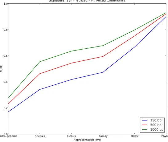
Chapter 4 deals with genomic signatures, which are functions frequently adopted by composition-based binning methods to have a vector space repre-sentation of the reads. A signature, in general, is a function that maps DNA sequences to points of a real vector space, consistently with the taxonomic clas-sification of their source organisms. In this chapter, we compare experimentally the performances of different genomic signatures on metagenomic data. New signatures are also studied; some of them capture the local deviation from the strand symmetry properties described by Chargaff’s second parity rule, while others exploit DNA symmetries to reduce the feature space dimension. Results indicate that it is possible to outperform the signature most commonly used in metagenomics while halving the feature space dimension.
A case study in metagenomics data annotation is described in Chapters 5 and 6. The related metagenomic project aims to study the anammox bacte-ria Candidatus ‘Brocadia fulgida’, sequencing the same community with three different technologies. In Chapter 5, in particular, we try to retrieve the core genes of anammox metabolism. This was done through BLASTX-based anno-tation of reads and assembled reads; these core genes were identified thanks to their similarity to the ones of Candidatus ‘Kuenenia stuttgartiensis’. Chapter 6 focuses on a comparative quantitative analysis of the metagenomes acquired by the three technologies: we investigate how well different technologies rep-resent information related to the considered organism of interest, and whether it is beneficial to combine information obtained through different technologies. BLASTX-based Open Reading Frame annotation of the metagenomes is ac-companied by a study of their content distributions. Annotation and GC-content analysis indicate that adjustments of sequencing protocols are desirable in order to prevent underrepresentation ofB. fulgida in the data. Results show that the combination of data obtained by different sequencing technologies can allow to recover relevant information of underrepresented organisms.
Material of this thesis was published in the following articles:
Journal Articles
• Gori, F., Folino, G., Jetten, M. S. M., and Marchiori, E. (2011b). MTR: taxonomic annotation of short metagenomic reads using clustering at multiple taxonomic ranks. Bioinformatics,27(2), 196–203
• Gori, F., Mavroeidis, D., Jetten, M. S. M., and Marchiori, E. (2012).
Genomic signatures for metagenomics: DNA symmetries matter. (under
review)
• Gori, F., Tringe, S. G., Kartal, B., Marchiori, E., and Jetten, M. S. M. (2011c). The metagenomic basis of anammox metabolism in Candidatus ‘Brocadia fulgida’. Biochemical Society Transactions,39(6), 1799–1804 • Gori, F., Tringe, S. G., Folino, G., van Hijum, S. A. F. T., Op den Camp,
H. J. M., Jetten, M. S. M., and Marchiori, E. (2013). Differences in se-quencing technologies improve the retrieval of anammox bacterial genome
from metagenomes. BMC Genomics,14, 7
Conference Articles
• Folino, G., Gori, F., Jetten, M. S. M., and Marchiori, E. (2009a). Clus-tering metagenome short reads using weighted proteins. In Evolution-ary Computation, Machine Learning and Data Mining in Bioinformatics,
volume 5483 ofLNCS, pages 152–163
• Folino, G., Gori, F., Jetten, M. S. M., and Marchiori, E. (2009b). Evidence-based clustering of reads and taxonomic analysis of metagenomic data. In Pattern Recognition in Bioinformatics, volume 5780 ofLNCS, pages 102–112
• Gori, F., Mavroeidis, D., Jetten, M. S. M., and Marchiori, E. (2011a). Genomic signatures for metagenomic data analysis: exploiting the reverse
complementarity of tetranucleotides. In Proceedings of the 5th IEEE
Similarity-based binning at
protein level
Binning methods aim to group reads into clusters in order to discover infor-mation about the composition of a microbial community. Here we focus on proxygenes methods, that are similarity-based binning methods that associate a protein (proxygene) to each cluster of reads; the proxygene is selected among the proteins identified by a sequence-similarity search. In this chapter we examine LWproxy, a well-known proxygene method present in literature, and we propose GWproxy, a new method that avoids the theoretical defects of LWproxy. The binning is performed by processing BLASTX-search output with combinatorial optimization methods. Experiments on benchmark datasets show the effective-ness of GWproxy for binning while maintaining a high accuracy of organism content.1
2.1
Introduction
The rapidly emerging field of metagenomics seeks to examine the genomic con-tent of communities of microbes to understand their roles and interactions in an ecosystem. Given the wide-ranging roles microbes play in many ecosys-tems, metagenomic studies will reveal insights into protein families and their evolution. Because most microbes cannot grow in the laboratory using cur-rent cultivation techniques, scientists have turned to cultivation-independent techniques to study microbial diversity. At first shotgun Sanger sequencing was used to acquire a metagenome, but nowadays massive parallel sequencing technologies, like 454 or Illumina, allow random sampling of DNA sequences to examine the genomic material present in a microbial community (Yooseph
1
This chapter contains parts of two publications: Folino, G., Gori, F., Jetten, M. S. M., and Marchiori, E. (2009a). Clustering metagenome short reads using weighted proteins. InEvolutionary Computation, Machine Learning and Data Mining in Bioinformatics, volume 5483 ofLNCS, pages 152–163. Folino, G., Gori, F., Jetten, M. S. M., and Marchiori, E. (2009b). Evidence-based clustering of reads and taxonomic analysis of metagenomic data. InPattern Recognition in Bioinformatics, volume 5780 ofLNCS, pages 102–112
et al., 2007).
For a given metagenome, one would like to determine the phylogenetic provenance of the obtained sequences, the relative abundance of its different members, their metabolic capabilities, and the functional properties of the community as a whole. To this end, computational analysis is becoming in-creasingly indispensable (McHardy and Rigoutsos, 2007; Raeset al., 2007). In particular, clustering methods are used for rapid analysis of sequence diversity and internal structure of the sampled community (Liet al., 2008), for discov-ering protein families present in the metagenome (Dalevi et al., 2008), and as a pre-processing step for performing comparative genome assembly (Pop
et al., 2004), where a reference closely related organism is employed to guide the assembly process.
In this chapter we focus on the problem of binning, that consists in clus-tering metagenomic reads according to their source proteins, genomes, or taxa (Dalevi et al., 2008; Li et al., 2008). Different methods for clustering analysis of metagenomic datasets have been proposed, that can be divided into two main approaches: composition-based and similarity-based methods. Composition-based methods directly compare the reads with each others using a similarity measure; this can be based, for instance, on sequence overlapping (Li et al., 2008) or on extracted features such as oligonucleotide frequency (Chan et al., 2008). Similarity-based methods employ knowledge extracted from external sources in the clustering process, like proteins identified by a sequence-alignment search (Dalevi et al., 2008).
Our approach is inspired by a similarity-based algorithm present in litera-ture (Dalevi et al., 2008), henceforth denominated as LWproxy, designed for clustering short reads. LWproxy is what we call a proxygenes method, a spe-cial type of similarity-based binning method: reads are clustered according to their source proteins, and a representative protein (proxygene) is associated to each cluster. The proxygene is selected among the proteins identified by a sequence-similarity search. Unfortunately, LWproxy has some significant the-oretical defects: we prove that results of LWproxy depend on the read selected at the beginning of the procedure, and two or more clusters might share the same proxygene.
We propose GWproxy, a new robust proxygenes method based on combina-torial optimization. The method performs automatic selection of the number of clusters, and generates possibly overlapping clusters of reads. While LWproxy clusters the reads and then chooses the proxygenes, GWproxy performs the two operations at the same time.
Specifically, GWproxy consists of three main steps. First, it uses a special-ized version of BLAST (Basic Local Alignment Search Tool), called BLASTX,
for aligning the reads of the metagenome to a reference protein database (Altschul et al., 1997). For each query read we obtain a list of similar pro-teins, calledhits; for each hit we extract two score values, calledbit-score and
identity-score, which measure the quality of the read-protein matching, and one confidence value, called E-value, which amounts to a confidence measure of the matching.
Next, a maximum ofK proteins for each read are selected, among those hits having E-value smaller than a given positive thresholdα. To each of these se-lected proteins a potential cluster of reads is associated; this set is made by the reads having the protein within their hits. The potential clusters are weighted by means of a novel measure based on the bit-scores and identity-scores, which assigns small weights to sets with high average-quality alignments.
Finally, the reads are clustered by translating the clustering problem into an instance of the weighted set covering problem (WSC). The WSC is a clas-sical constrained optimization problem used in many real-life applications. In this case, the problem consists in selecting the minimum total weight collec-tion of potential clusters such that each read belongs to at least one cluster. We employ a publicly available fast heuristic algorithm for the weighted set covering problem (Marchiori and Steenbeek, 2000). The resulting clustering method generates a set of clusters, where each cluster is represented by the associated protein, namely the proxygene.
In order to assess the effectiveness and benefits of GWproxy, we consider the metagenomic datasets introduced in (Daleviet al., 2008). We measure the quality of the resulting clusters by means of the number of clusters, their car-dinality, the total overlapping, and the homogeneity of their organism content (Li et al., 2008).
Specifically, we analyze the behavior of GWproxy when varying its param-etersKandα. Results show that the number of clusters decreases when larger values of K are chosen, while their overlapping increases. The organism con-tent of the clusters does not change substantially for higher values of K and fixed α (equal to 0.01), indicating the effectiveness of the proposed approach in clustering a metagenome while maintaining a high homogeneity of organism content within each cluster.
2.2
Methods
In this section we revise the binning method introduced in (Dalevi et al., 2008), here called LWproxy, and we describe GWproxy, the new method we developed. Both are proxygenes method: their outputs are clusters of reads and a protein is associated to each cluster. These proteins, called
proxy-genes, are chosen to be good representatives of the associated clusters of reads. More formally, a proxygenes method generates a collection of kpairs (Ci, gi),
i= 1, . . . , k;Ci is a set of reads and gi is the protein associated toCi
(proxy-gene).
Here and in the sequel we assume that reads of the metagenomic dataset were aligned to the proteins of a given reference database. The alignments were performed by BLASTX, and a cutoff α ∈R+ for alignmentE-value was
given by the user (for a detailed description of BLASTX, see Appendix A).
We denote by R the resulting set of reads having at least one BLASTX hit
satisfying the given cutoff, and by P the set of proteins occurring in the hits of at least one read ofR.
2.2.1 LWproxy
LWproxy clusters the readsR using the aligned proteinsP withE-value cutoff
α; it also exploits the bit-scoresSB of the read-protein alignments (for a
de-tailed description of bit-score, see Appendix A). The main part of the algorithm can be summarized as follows.
1. Seti= 0. 2. SetX =R.
3. IfX is empty, then terminate; otherwise seti=i+ 1.
4. Select randomly2 one read ˜r from X as seed of clusterCi ={r˜}. 5. Remove ˜r from X.
6. SetHi to the set of hits of ˜r.
7. Add to Ci all the reads having one element of Hi as the first hit, called
best hit, and remove them fromX.
8. Add to Hi all hits of those reads added toCi in the previous step. 9. If no reads are added, then go to step 3; otherwise go to step 7.
When the clustering process is terminated, the method assigns one proxygene
gi to eachCi by selecting from Hi the protein having highest cumulative
bit-score. Algorithm 1 gives a more formal description of LWproxy. The Example 1 shows how LWproxy works on a toy problem. 2
We consider here random seed selection. However, in (Daleviet al., 2008) the criterion for selecting a seed is not specified.
Algorithm 1 LWproxy algorithm
Input: Set of readsRhaving at least one BLASTX alignment withE-value≤
α; set of proteinsP to which readsRhave a significant BLASTX alignment; set of bit-scores{SB(r, p)|r∈R, p∈P}, whereSB(r, p) := bit-score of the
alignment between readr and protein p.
Output: Clusters of reads C1, . . . , Ck s.t. ∪ki=1Ci = R and Ci ∩ Cj = ∅,
∀i, j= 1, . . . , k,i6=j; proteins p1, . . . , pk s.t. pi is the proxygene ofCi. i←0
X←R
whileX 6=∅ do i←i+ 1 select ˜r∈X
D← {˜r} {D contains the reads to be processed}
X←X\D
Ci←D
Q← {p∈P |p is a hit of ˜r}
Hi←Q {Qcontains the proteins to be processed}
while D6=∅ do
D←S
p∈Q{r ∈X|pis the best hit of r} if D6=∅ then X←X\D Ci ←Ci∪D Q←S r∈D{p∈P |pis a hit of r} Hi ←Hi∪Q end if end while return Ci pi ←argmaxp∈Hi P r∈CiSB(r, p) return pi end while
Example 1 Suppose that five reads R := {r1, . . . , r5}, and eight aligned
pro-teins P := {p1, . . . , p8} are given. Here is the list of the hits for each read
(bit-score of the hits are in brackets):
• r1 :{p1(30), p3(20), p5(10)}
• r2 :{p3(30), p4(20), p2(10)}
• r3 :{p5(50), p2(20), p6(10)}
• r4 :{p7(40), p5(30), p8(10)}
• r5 :{p8(40), p5(30), p7(10)}
If LWproxy selects r4 as seed for the first cluster C1, then reads r3 and r5
will be added to C1, since p3 and p5 are their best hits, respectively. This
first cluster cannot be ulteriorly expanded, so that C1 ={r3, r4, r5} and H1 =
{p2, p5, p6, p7, p8}. Now the algorithm selects a new seed among the remaining
reads {r1, r2} to build up a new cluster C2. Whatever the seed is, the cluster
C2 is going to become the set {r1, r2}; H2 is the set {p1, p2, p3, p4, p5}. The
proxygenes of clusters C1 and C2 arep5 andp3, respectively.
LWproxy Drawbacks
The main drawback of LWproxy is that results may be affected by the choice of the seed read used in the first step of the algorithm. Example 2 illustrates that a different clustering will be obtained by LWproxy on the toy problem in Example 1 if another seed read is selected.
Example 2 Consider the toy problem in Example 1. Suppose LWproxy selects r2 as seed of the first cluster C1. Since its hits (p2, p3, and p4) are not best
hits of any other read, no reads are added and consequently the proxygene of C1 = {r2} is the best hit of r2, namely the protein p3. Even the clusters C2
and C3 are singleton sets if reads r3 and r1 are selected as second and third
seeds, respectively. The proxygenes of clusters C2 = {r3} and C3 = {r1} are
therefore p5 and p1, respectively. The last cluster C4 ={r4, r5} has proxygene
p5 and is obtained whatever its seed read is.
Secondly, Example 3 shows that the same proxygene can be assigned to more than one cluster. As described in (Dalevi et al., 2008), a proxygene of a cluster is a protein that has been chosen to represent the reads of that cluster. Consequently, if two or more clusters share the same proxygene, it means that these clusters had to be merged in a unique cluster; however, this task is not performed by LWproxy.
Example 3 Consider the toy problem in Example 1. Suppose LWproxy selects r1 as seed of the first cluster C1. Its hits arep1, p3 and p5, so that readsr2 and
r3 are added to C1. The proxygene associated to C1 is p5, because it has the
highest cumulative bit-score. As it happened in Example 2, the remaining reads r4 andr5 are grouped together in the second and last cluster C2, irrespectively
of the selected seed. Both clusters have the same proxygene p5.
2.2.2 GWproxy
To overcome the drawbacks of LWproxy, we propose a new proxygenes method called GWproxy; this method performs automatic selection of the number of clusters, and generates possibly overlapping clusters of reads. The binning is performed processing BLASTX-search output to generate an instance of Weighted Set Covering, a classical combinatorial optimization problem. The final clustering is given by the solution of this problem.
GWproxy has two parameters: theE-value cutoffαand the number-of-hits cutoff K. The parameter K is used as a secondary cutoff for alignment sig-nificance. First, the BLASTX-search output is processed to assign a potential clusters Cj with weightwj to each protein pj. Let R := {r1, . . . , rm} be the
set of the reads with a feasible BLASTX alignment (E-value ≤α) to proteins
P := {p1, . . . , pn}. The potential cluster Cj associated to pj is made by all
the reads ofR having pi within the first K BLASTX hits. Aweight wj ∈R+
is assigned to each potential clusterCj. The weightwj is in inverse proportion to the average quality of the alignments between pj and the reads of Cj; it is
defined as follows wj := 1 + 1 |Cj| X r∈Cj 100S max B −SB(r, pj)
SBmax−SBmin + 100−Id(r, pj) ,
where Id(r, p) and SB(r, p) denote the identity and the bit-score of the
align-ment between read r and protein p, respectively (for a detailed descriptions of these two scores, see Appendix A). SBmin and SBmax are the minimum and maximum bit-score over all hits relative to the proteins inP, respectively. |Cj|
is the cardinality ofCj (number of elements ofCj); the symboldvedenotes the ceiling function, that maps a real number v to the smallest following integer (dve:= min{z∈Z|z≥v}).
The clustering is obtained by selecting a family C of potential clusters
Cj1, . . . , Cjk among the ones previously defined. The clusters that compose C
are chosen such that each read of Ris contained in at least one of the clusters ofC and the sum of the weights of the selected clusters, that iswj1+. . .+wjk,
is minimal. The proteins associated to C, namely pj1, . . . , pjk, are the chosen
proxygenes.
The task of choosing the elements ofC is cast as an instance of the classic
Weighted Set Covering problem, (WSC), one of the oldest and best studied NP-hard problems. Given a collection of weighted sets Z1, . . . , Zn with U :=
∪n
i=1Zi, the WSC consists in finding the minimum total weight sub-collection
Zj1, . . . , Zjk satisfying the constraint∪
k
i=1Zji =U. Our task, being an instance
of WSC, can be formulated as an integer linear program:
min x∈{0,1}n n X j=1 xjwj, s.t. n X j=1 aijxj ≥1, for i= 1, . . . , m, (WSC)
where the matrix A∈ {0,1}m×n is s.t.
aij =
(
1, ifri∈Cj, 0, otherwise,
and the binary variable xj indicates whether a potential clusterCj belongs to the solution (xj = 1) or not (xj = 0). The m constraint inequalities express
the requirement that each read ri ∈R belongs to at least one of the selected
Cj. Hence, if ¯x ∈ {0,1}n indicates the solution of WSC, than the clustering obtained, namely C, is made by all the potential clusters Cj s.t. x¯j = 1.
To achieve a solution in an adequate time, we use a fast heuristic algorithm3 for WSC originally developed for tackling airline crew scheduling problems (Marchiori and Steenbeek, 2000).
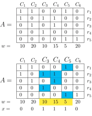
Table 2.1 and Table 2.2 illustrate the application of the procedure to a toy example. Suppose that the BLASTX search of R = {r1, . . . , r5} against
a given protein database gives the hits shown in Table 2.1. Table 2.2 (top) shows the matrix A ∈ {0,1}5×6 and the vector of weights w derived from such BLASTX results. The WSC algorithm, applied to this problem instance, selects the clusters C3 ={r2, r4},C4 ={r2, r3}, andC5 ={r2, r3}; every read
is contained in at least one cluster (C3∪C4∪C5 =R) and the total weight is
30 (see the bottom of Table 2.2).
2.3
Experiments
We considered three simulated metagenomic datasets introduced in (Dalevi
et al., 2008), called in the following M1, M2 and M3. These datasets were generated from 9, 5 and 8 genome projects, respectively. The genomes were
3
Table 2.1: Hits of Reads to proteins identified with BLASTX for a toy example: rowicontains the hits for readri(left), the relative potential clusters (center), and weights (right).
r1 p1 p2 p5 r2 p1 p3 p4 r3 p2 p4 r4 p3 r5 p5 p6 C1 = {r1, r2}, C2 = {r1, r3}, C3 = {r2, r4}, C4 = {r2, r3}, C5 = {r1, r5}, C6 = {r5}, w1 = 10 w2 = 20 w3 = 10 w4 = 15 w5 = 5 w6 = 20
sequenced at the Joint Genome Institute (JGI) using the 454 GS20
pyrose-quencing platform that produces ∼100 bp reads. From each genome project,
reads were sampled randomly at coverage level 0.1X. The coverage is defined as the average number of times a nucleotide is sampled. The resulting datasets M1, M2 and M3 consisted of 35,230, 28,870 and 35,861 reads, respectively. Ta-ble 2.3 shows the names of the organisms and the number of reads generated for the M1 dataset; for the composition of datasets M2 and M3, see Appendix Ta-ble C.1. The reader is referred to (Daleviet al., 2008) for a detailed description of all the datasets. As a reference database for our BLASTX alignments we
used the NCBI-NR4 (non-redundant) protein sequence database downloaded
on October 2008 (for a description of NCBI-NR, see Appendix A).
For the external softwares we used, that are BLASTX and the WSC solver, the following parameters were chosen. For BLASTX, the default parameters were used. The WSC solver was run with pre-processing (-p) and number of it-erations equal to 1,000 (-x1000); 150 sets were selected for building the starting partial solution at the first iteration (-b150) and, at each following iteration, one tenth of the sets forming the best solution obtained in the previous itera-tions were used as a starting partial solution (-a0.1). We refer to (Marchiori and Steenbeek, 2000) for a detailed description of the WSC program.
2.3.1 Evaluation
First we set the E-value cutoff α to a reasonable value, equal to 0.01. Not every read had a feasible alignment, because some reads had only alignments with E-value above α. This resulted in the selection of 21,236 reads for M1,
4
Table 2.2: (Top) Input covering matrix; position (i, j) contains 1 if proteinpj
is a hit of read ri, otherwise it contains 0. (Bottom) The proteins and read clusters selected by the WSC algorithm.
C1 C2 C3 C4 C5 C6
A
=
1 1 0 0 1 0 r1 1 0 1 1 0 0 r2 0 1 0 1 0 0 r3 0 0 1 0 0 0 r4 0 0 0 0 1 1 r5 w= 10 20 10 15 5 20 C1 C2C
3C
4C
5 C6A
=
1 1 0 0 1 0 r1 1 0 1 1 0 0 r2 0 1 0 1 0 0 r3 0 0 1 0 0 0 r4 0 0 0 0 1 1 r5 w= 10 20 10 15 5 20 x= 0 0 1 1 1 0Table 2.3: Characteristics of the simulated data: identifier and name of the organism, size of its genome and total number of reads sampled for coverage 0.1X (M1 dataset). Detailed information on these datasets can be found in (Dalevi et al., 2008).
Organism Genome size (bp) Reads sampled
Clostridium phytofermentansISDg 4,533,512 4,638
Prochlorococcus marinusNATL2A 1,842,899 1,866
Lactobacillus reuteri100-23 2,174,299 2,371
Caldicellulosiruptor saccharolyticusDSM 8903 2,970,275 2,950
Clostridium sp. OhILAs 2,997,608 2,934
Herpetosiphon aurantiacusATCC 23779 6,605,151 6,937
Bacillus weihenstephanensisKBAB4 5,602,503 4,158
Halothermothrix oreniiH 168 2,578,146 2,698
21,064 for M2, and 24,043 for M3, respectively.
We analyzed the different clusterings we obtained by varying the value of
K (1, 2, 10, 50, and 1,000) with respect to the following features:
• The number ofselected proteinsP, that are the proteins having a feasible BLASTX alignment to the selected reads R;
• The number of clusters obtained and their cardinalities (number of ele-ments of a cluster);
• The total clusters overlapping, defined as the sum of the cardinalities of the clusters minus the number of selected reads;
• The reduction factor, defined as the number of selected reads divided by the number of clusters;
• The homogeneity of the organism content of the clusters. This was mea-sured by the so-called cluster purity: for a given cluster, it is defined as the relative abundance of the most abundant organism in the cluster. This is the ratio between the number of reads belonging to the most abundant organism in the cluster and cluster cardinality.
A similar analysis was performed by fixingK to a reasonable value, equal to 50, and varying the parameter α. The studied values of α were 0.1, 0.01, 0.001, 0.0001, and 10−6.
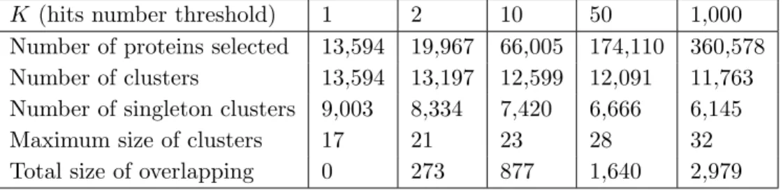
2.3.2 Results: fixed value of α = 0.01 and varying K values Table 2.4 summarizes the results for dataset M1, setting αto 0.01 and varying
K values. The number of selected proteins increased whenK increased, while the number of clusters decreased, indicating effectiveness of GWproxy to select proxygenes. Furthermore, the number of singleton clusters also decreased for higher values of K, indicating an increasing clustering capacity of GWproxy. A similar trend can be observed for datasets M2 and M3 (Appendix Tables B.1, B.2).
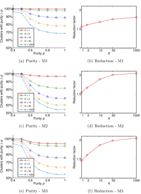
Subfigures 2.1(a), 2.1(c), and 2.1(e) show, for each datasets, the percentage of non-singleton clusters having purity greater or equal than a given value p, for selected values of p ∈ [0.4,1]. For all the datasets, the curve at K = 1 dominates all the other ones, justified by the fact that the corresponding clustering contained many clusters of small size, that are likely to have higher purity. For instance, for the M1 dataset, setting K= 1 andK = 1,000, about 75% and 35% of the clusters had size equal to 2, respectively. Subfigures 2.1(b), 2.1(d), and 2.1(f) show, for each dataset, the reduction factor for different
Table 2.4: Summary of the results of experiments for α = 0.01 and varying
parameterK (M1 dataset).
K (hits number threshold) 1 2 10 50 1,000
Number of proteins selected 13,594 19,967 66,005 174,110 360,578
Number of clusters 13,594 13,197 12,599 12,091 11,763
Number of singleton clusters 9,003 8,334 7,420 6,666 6,145
Maximum size of clusters 17 21 23 28 32
Total size of overlapping 0 273 877 1,640 2,979
values ofK. As expected, a larger value ofK resulted into a higher reduction factor.
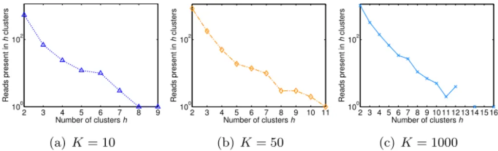
Finally, Figure 2.2 shows, for dataset M1, how the number of reads occur-ring in more than a given number of clusters varied for different choices ofK. For a small value ofK (equal to 10) each read belonged to at most 9 clusters, while for a very high value ofK (equal to 1,000) each read occurred in at most 16 clusters. Indeed, as reported in Table 2.4, the total overlapping showed a substantial increase for high values ofK. These results can be due to the fact thatK is an upper bound on the maximum number of clusters that a read may belong to. Similar results were obtained using M2 and M3 datasets (Appendix Figures B.1 and B.2).
2.3.3 Results: fixed value of K = 50 and varying α values.
Table 2.5: Summary of the results of experiments for K= 50 and varying the
E-value threshold α (M1 dataset).
α (E-value threshold) 0.1 0.01 0.001 0.0001 10−6
Number of reads selected 22,219 21,236 20,300 19,085 16,736
Number of proteins selected 208,443 174,110 146,524 116,682 72,149
Number of clusters 12,283 12,091 11,850 11,534 10,660
Number of singleton clusters 6,464 6,666 6,772 6,889 6,801
Maximum size of clusters 30 28 27 23 19
Total size of overlapping 2,026 1,640 1,326 1,066 528
vary-0.4 0.6 0.8 1 50% 60% 70% 80% 90% 100% Purity p
Clusters with purity
≥ p K = 1 K = 2 K = 10 K = 50 K = 1000 (a) Purity - M1 1 2 10 50 1000 1 1.5 2 K Reduction factor (b) Reduction - M1 0.4 0.6 0.8 1 50% 60% 70% 80% 90% 100% Purity p
Clusters with purity
≥ p K = 1 K = 2 K = 10 K = 50 K = 1000 (c) Purity - M2 1 2 10 50 1000 1 1.5 2 K Reduction factor (d) Reduction - M2 0.4 0.6 0.8 1 50% 60% 70% 80% 90% 100% Purity p
Clusters with purity
≥ p K = 1 K = 2 K = 10 K = 50 K = 1000 (e) Purity - M3 1 2 10 50 1000 1 1.5 2 K Reduction factor (f) Reduction - M3
Figure 2.1: (a),(c),(e): plots of percentage of non-singleton clusters with purity ≥ p for different values of K, for M1, M2 and M3, respectively. (b),(d),(f): plots of the reduction factor for different values of K, for M1, M2 and M3, respectively.
2 3 4 5 6 7 8 9 100 102 Number of clusters h Reads present in h clusters (a)K= 10 2 3 4 5 6 7 8 9 10 11 100 102 Number of clusters h Reads present in h clusters (b) K= 50 2 3 4 5 6 7 8 9 10 11 12 13 14 15 16 100 102 Number of clusters h Reads present in h clusters (c)K= 1000
Figure 2.2: Plot of the number of reads occurring in h different clusters (M1 dataset).
ingαvalues. Higher values ofαresulted into the selection of an higher number of reads and of proteins. Moreover, overlapping and cluster size increased with
α. Similar remarks hold also for the results obtained for M2 and M3 (Appendix Tables B.3 and B.4).
The plots of Figure 2.3 show that, on the M1 dataset, small values of α
led to clusterings with a reduction factor of about 1.6 and where 90% of the clusters were very accurate, in terms of organism content. For larger values of
α, clusters’ purity decreased up to about 75%, while reduction factor increased reaching a maximum of about 1.8. Similar results were obtained for datasets M2 and M3 (Appendix Figure B.3). Thus, the user of GWproxy can choose the trade-off between purity and reduction, depending on the specific research question to be addressed. 0.4 0.6 0.8 1 50% 60% 70% 80% 90% 100% Purity p
Clusters with purity
≥ p E−value=0.000001 E−value=0.0001 E−value=0.001 E−value=0.01 E−value=0.1 (a) 1e−061 0.0001 0.001 0.01 0.1 1.5 2 E−value Reduction factor (b)
Figure 2.3: a) plot of percentage of non-singleton clusters with purity ≥pfor different values of α. b) plot of the reduction factor for different values of α
2.4
Conclusions and Future Work
This chapter introduced GWproxy, a new proxygenes method for short reads, and analysed its performance on benchmark metagenomic datasets. We fo-cussed on the experimental analysis of the two parameters of GWproxy, namely
K and α. Results indicate the effectiveness of GWproxy as a tool for binning metagenomic data.
Regarding the computational cost of GWproxy, the algorithm we used is very efficient, due to the fast heuristic employed to search for an optimal set cover of the WSC instance. The running time is dominated by computationally-expensive BLASTX search performed at the beginning, that we used for align-ing the reads to the reference proteins. This is a common problem among similarity-based binning methods. Nevertheless, the aligning process can be parallelized by partitioning the set of reads and running BLASTX indepen-dently on each element of the partition.
In the future, we intend to investigate in more depth the biological meaning of the resulting clusters, in particular their functional and taxonomic content, in order to discover knowledge related to the protein content and the taxonomic organization of the organisms contained in the metagenome.
Moreover, similar experiments on data with higher coverage could be per-formed, and analyses with more sophisticated measures of cluster homogene-ity, like Normalized Mutual Information and Entropy Correlation Coefficient (Pluim et al., 2000) could be conducted.
Similarity-based binning at
multiple taxonomic ranks
One interesting problem in metagenomic data analysis is the discovery of the taxonomic composition of a given dataset. A simple method for this task, called the Lowest Common Ancestor (LCA), is employed in state-of-the-art computational tools for metagenomic data analysis of very short reads (about 100 bp). However LCA has two main drawbacks: it possibly assigns many reads to high taxonomic ranks and it discards a high number of reads. We present MTR, a new method for tackling these drawbacks using clustering at Multiple Taxonomic Ranks. Unlike LCA, which processes the reads one-by-one, MTR exploits information shared by reads. Results of experiments show that MTR improves on LCA by discarding a significantly smaller number of reads and by assigning much more reads at lower taxonomic ranks. Moreover, MTR provides a more faithful taxonomic characterization of the metagenome population distribution.1
3.1
Introduction
New sequencing technologies and the dramatic reduction in the cost of se-quencing have boosted the development of metagenomics, a new discipline that studies DNA and RNA sequences sampled from genomic material present in a microbial community (Yooseph et al., 2007). Metagenomics has gained pop-ularity because it allows researchers to study (the large amount of) microbes that cannot be cultured (Amannet al., 1995) and their role in the environment, for instance in terms of interaction with other organisms. Sequencing a sample produces a collection of DNA or RNA sequences, calledreads, belonging to the different genomes present in the sample. Ametagenomic dataset is a collection of these sampled reads.
1
This chapter is based on: Gori, F., Folino, G., Jetten, M. S. M., and Marchiori, E. (2011b). MTR: taxonomic annotation of short metagenomic reads using clustering at multiple taxonomic ranks.Bioinformatics,27(2), 196–203
Until recently shotgun Sanger sequencing was the main technology used in metagenomics (Sanger and Coulson, 1975; Sanger et al., 1977), producing reads of length ranging between 800 and 1000 base pairs (bp). Nowadays, other less expensive technologies like Roche 454 (Margulieset al., 2005) and Illumina platforms2 generate reads of 100-400 bp and 75-100 bp, respectively. Such new sequencing technologies produce very large datasets containing short reads. Computational analysis techniques are indispensable to extract knowledge from these datasets (McHardy and Rigoutsos, 2007; Raeset al., 2007; Kuninet al., 2008; Qin et al., 2010).
This chapter deals with binning, a common approach used to understand the content of a metagenome. Binning consists in clustering the reads accord-ing to their source proteins, genomes, or taxa. Computational approaches for binning can be divided into two main groups: composition-basedand similarity-based. Composition-based binning methods cluster the reads according to their GC-content, codon usage and other oligonucleotide frequencies. These methods cannot be directly applied to short reads because of the local variation of nu-cleotides distribution across a genome (Bentley and Parkhill, 2004). Moreover, external environmental factors seem to influence the GC nucleotide compo-sition of a community, suggesting that it may be even harder to distinguish the reads of different organisms relying on GC-content (Foerstneret al., 2005). Similarity-based binning methods assign reads to proteins, organisms or taxa using similarities of reads to reference sequences of a given database. Simi-larity is usually measured by means of sequence alignment tools, like BLAST (Altschul et al., 1997). This approach is useful when most reads in the sam-ple have significant similarities to reference sequences from known operational taxonomic units (Wooley et al., 2010). The incompleteness of the informa-tion contained in reference databases and the bias towards cultivable species constitute inherent limitations of the similarity-based approach. Nevertheless, similarity-based techniques have been shown to be effective for the taxonomic analysis of metagenomes (Husonet al., 2007; Daleviet al., 2008). Furthermore, results of ongoing projects on sequencing reference genomes will likely produce many more reference data available in the near future (Turnbaughet al., 2007). In this chapter we focus on the taxonomic assignment of very short reads (about 100 bp) to putative taxa. Taxonomic assignment is a special type of similarity-based binning: each read is assigned to a known taxon present in a reference taxonomic tree. Reads can be assigned to taxa belonging to different ranks.
A simple algorithm for taxonomic assignment is the Lowest Common
An-2
cestor (LCA) (Wang et al., 2007; Liu et al., 2008). LCA is the core algorithm of MEGAN (Huson et al., 2007) and of the Galaxy (Blankenberget al., 2007, 2010) web-based annotation tool3; also CARMA (Krauseet al., 2008) is based on an algorithm somewhat similar to LCA. CARMA identifies protein family sequences among the reads and it assigns each sequence to the ancestor taxon shared by the phylogenetic subtree of reference proteins where the sequence is located. LCA assigns to each read one taxon computed by means of the least common taxonomic ancestor of a suitable set of reference sequences (hits). These hits are obtained by matching the read against a database of reference sequences, like the NCBI-NR protein database, using BLASTX or other se-quence alignment tools. In this way LCA assigns reads to taxa at possibly different taxonomic ranks.
Two limitations of LCA rise from the way in which taxonomic information from matching reference sequences is combined. (1) LCA annotates a relatively small percentage of reads because a read is discarded if the least common taxon of its hits cannot be computed; (2) LCA assigns many reads to taxa at high ranks, because it computes the lowest common ancestor of (possibly many) matching sequences (Kunin et al., 2008). The first limitation is addressed by methods that assign all reads. The simplest and most used of such meth-ods assigns each read to its best matching reference sequence according to BLASTX, called Best Hit (BH); as recently shown for instance in (Brady and Salzberg, 2009), this is still the best stand-alone assignment method for long reads (of length 800 bp or more). A more involved method assigning all reads is Phymm (Brady and Salzberg, 2009). In Phymm a classifier is trained based on interpolated Markov models on a large amount of curated genomes. This classifier constructs probability distributions representing observed patterns of nucleotides that characterize each chromosome or plasmid. On metagenomic datasets with long reads (800 bp and 1,000 bp) Phymm was shown to outper-form BH at ranks Class and Phylum. The authors also showed that a suitable combination of BH and Phymm (called PhymmBL) significantly improved ac-curacy of both BH and Phymm. However, acac-curacy of PhymmBL for short reads (100 bp) remains rather low, ranging from 58.5% at rank Genus to 77.5% at rank Phylum. The second drawback of LCA, that is, the fact that it assigns many reads to taxa at high ranks, has been recently tackled in (Clementeet al., 2010), where a method was proposed for assigning each read to a taxon at a rank lower (or equal) than the one selected by LCA. The choice of such taxon is based on the number of mismatches between the read and the organisms in that taxon.
3
LCA is present in Galaxy Metagenomic Analyses tools by the name “lowest diagnostic rank”.
To overcome both drawbacks of LCA we introduce an algorithm for the taxonomic assignment of reads. Our approach is motivated by the following observations. LCA uses taxonomic information of matching reference sequences locally, that is, the taxonomic assignment of each read is performed indepen-dently of the other ones. However, reads of a metagenome are related among each other. In particular, groups of reads have common matching reference se-quences. We propose to use this global type of information to design a new tax-onomic assignment algorithm, called MTR (Multiple Taxtax-onomic Ranks based clustering). MTR performs the following two steps at each taxonomic rank. First, taxonomic information shared by reads at that rank is used for charac-terizing clusters of reads having the same taxon. Next, a ”best” subset of the resulting clusters is selected. Such selection task is casted into a combinato-rial optimization problem and solved using an existing efficient approximation algorithm. This global optimization method for grouping reads into clusters having a common taxa produces multiple taxonomic assignments, one for each rank. However, the taxons assigned to a read at different ranks may be in-consistent with each others. We solve such inconsistencies by assigning each read to a taxon at lowest rank such that the multiple taxonomic assignments of that read from the highest to the selected rank form a consistent taxonomic lineage.
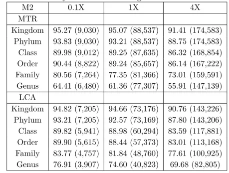
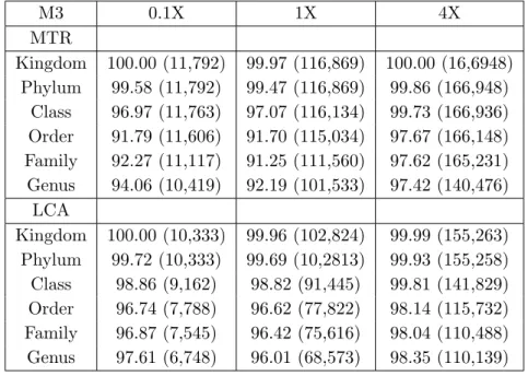
We demonstrate the effectiveness of this approach on several metagenomic datasets, both simulated and real-life. On all the considered datasets, MTR discards a significantly smaller number of reads than LCA and it assigns much more reads at lower taxonomic ranks. Furthermore, on simulated metagenomes M1, M2 and M3, MTR is shown to provide a more faithful taxonomic char-acterization of the population distribution than LCA. With respect to the correctness of the assignments, both LCA and MTR’s accuracy appears to re-flect the difference in taxonomic composition of the simulated datasets, with M1 composed of representatives of less well-sampled phyla (i.e. less present in the reference data) than M2 and M3 (Dalevi et al., 2008). Nevertheless, results indicate that MTR is capable to assign a read to a taxon similar to the true one, when the true taxon does not occur among (the taxa of) its hits. In general, our experimental investigation indicates that MTR provides an effec-tive method for performing taxonomic analysis of a metagenomic dataset with short reads.
3.2
Methods
We propose a method for taxonomic assignment of short reads motivated and inspired by LCA (Husonet al., 2007). In LCA a read is compared, usually with
BLASTX, against a database of reference sequences, such as the NCBI-NR protein database, and the taxonomic information of significant matches, called
hits, is extracted and mapped onto the leaves of the NCBI taxonomy. The
leaves of the NCBI taxonomy represent different species and strains. LCA computes the lowest common ancestor of all these hits, which corresponds to some higher-rank taxon, and will then assign the read to that taxon. In this way, species-specific sequences are assigned to the leaves, whereas sequences that are conserved among different species, or that are susceptible to horizontal gene transfer, are assigned to taxa of less-specific ranks.
Observe that LCA processes each read independently, hence it does not use taxonomic information shared by alignments of different reads. However, each read is related to other reads, because the metagenome is the union of disjoint sets of reads, each one sequenced from a different organism. Therefore we propose to use information shared among reads for developing the following global taxonomic assignment method, called MTR.
3.2.1 Read Assignment at Multiple Taxonomic Ranks
Like in LCA, all reads are submitted as BLASTX queries against a protein sequence database and proteins of high-quality alignments are selected (for a detailed description of BLASTX, see Appendix A). This process generates one set of protein hits for each read. The taxonomic information of these proteins is used by MTR for clustering reads at each taxonomic rank such that reads in the same group are assigned to the same taxon at that rank.
Specifically, letRbe the set of reads having at least one high-quality align-ment, and let r denote a read. For each taxonomic rank, from the highest to the lowest, each readris either assigned to a taxon at that rank or is considered not assigned at that and lower taxonomic ranks. The latter case happens if the taxonomic assignment of r at that rank is not consistent with its assignments computed at higher ranks. In that caser is removed fromR. Thisconsistency test is performed at each rank (see step 3 below).
Taxonomic assignment at a given taxonomic rank is performed using a clustering approach. Here we view clustering as the problem of searching for a minimum family of possibly overlapping clusters of reads whose union is the considered set of reads. To this aim we define an ad-hoc search space and search strategy. The search space consists of clusters of reads directly characterized using the taxa of proteins of those high-quality alignments that are obtained by submitting the reads as BLASTX queries. The search strategy is based on combinatorial optimization. The search space construction procedure, search strategy and consistency test are described in detail below.
1. Search space construction: generate clusters of reads using the taxa of their hits. MTR generates a collection of clusters of reads, where each cluster is associated to a taxon at the considered rank. A cluster Cj
consists of those reads inRhaving a high-quality alignment with at least one protein having taxonj.
2. Search strategy: select an optimal family of clusters. The algorithm se-lects a minimum family of clusters that together contain all the consid-ered reads. This selection task is casted into a combinatorial optimization
problem, theSet Covering Problem (SCP):
arg min
J⊆{1,...,n}|J|, such that ∪j∈JCj =R. (SCP)
Here n is the total number of clusters generated at Step 1. This ap-proach is inspired by previous works for clustering reads using proxygenes (Dalevi et al., 2008; Folino et al., 2009a) (see Chapter 2). The program used by MTR for solving (heuristically) the SCP is an implementation of the greedy set covering algorithm (Chv´atal, 1979). This is a very simple greedy algorithm that, at each stage, chooses the set containing the largest number of elements that do not belong to any of the clusters selected so far (Algorithm 2). The greedy algorithm can be efficiently implemented in time that is linear in the size of the input (Bar-Yehuda and Even, 1981).
Algorithm 2 Greedy algorithm for Set Covering (Chv´atal, 1979)
Input: Family of sets C1, . . . , Cn;R:=∪nk=1Ck.
Output: J ⊆ {1, . . . , n}, s.t. ∪j∈JCj =R. U ←R J ← ∅ while U 6=∅do select ˆi∈ {1, . . . , n} \J s.t. |Cˆi∩U|is maximum U ←U \Cˆi J ←J∪ {ˆi} end while return J
The selection process is illustrated by means of the following toy example. Suppose we have ten reads, R ={r1, . . . , r10}. For each read, the taxa
(left). A bullet in entry (i, j) indicates that read ri belongs to cluster
Cj; this means that if Cj is selected, ri will be assigned to taxon j. The problem is to select a minimum number of clusters (columns of that matrix) whose union contains all the ten reads. A solution is shown in the figure on the right-hand side of Table 3.1, where the selected clusters areC1,C2 and C5. Therefore, the reads are assigned to taxa 1, 2 and 5.
3. Consistency test. For each read inR, MTR now checks that its taxonomic assignment at this rank is consistent with its taxonomic assignments com-puted at higher ranks. That is, if read r has been assigned to taxon j
at the considered rank, we check that at higher ranksr was assigned to ancestors of taxonj. If this does not happen, thenr is not assigned from that rank onwards and is removed fromR.
Table 3.1: Left: input covering matrix. Right: a solution of the SCP.
C1 C2 C3 C4 C5 C6 r1 • • • r2 • • r3 • • r4 • • • r5 • • r6 • • r7 • • • r8 • • r9 • • r10 • • C1 C2 C3 C4 C5 C6 r1 • • • r2 • • r3 • • r4 • • • r5 • • r6 • • r7 • • • r8 • • r9 • • r10 • •
Observe that, at a given rank, MTR can assign a read to more than one cluster. This is illustrated in our toy example where, for instance, read r2 is
assigned to clusters C2 and C5. However we want to assign a unique
taxon/-cluster to each read. Therefore MTR assigns each read r to the largest cluster among those containing r (ties are broken randomly), while keeping the tax-onomical consistency of the assignments of r at different ranks. For instance, read r2 will be assigned to C5. The final assignment computed by MTR
as-sociates each read r in R to the taxon (cluster) containing r and having the lowest rank.
Both LCA and MTR process a set of hits computed using BLAST and output a read-taxon assignment, where reads are possibly assigned to taxa at different taxonomic ranks. MTR and LCA are also similar in that they output the same taxon for each read that is assigned by both methods at the same taxonomic rank. In fact, if a read r is assigned by both methods at the same
rank it means that that rank contains the lowest common ancestor taxon of the hits of r. At that rank r is associated to only one taxon, therefore MTR will be forced to assignr to that taxon.
The running time of both MTR and LCA is dominated by the alignment of reads with the reference protein sequences database using BLASTX. This is a computational bottleneck common to similarity-based methods for metage-nomic analysis based on the alignment of reads with sequences of a large database of reference.
3.3
Experiments
3.3.1 Data
We analyzed nine simulated and three real-life metagenomic datasets. The nine simulated datasets had been derived from three sets of organisms, here denoted by M1, M2 and M3; these datasets had been introduced in (Daleviet al., 2008). M1, M2 and M3 were composed by 9, 5 and 8 distinct genomes, respectively. These genomes had been sequenced at the Joint Genome Institute (JGI) using
the 454 GS20 pyrosequencing platform that produces ∼ 100 bp reads. From
each set of organisms, reads had been randomly sampled at three different levels of coverage (0.1X, 1X and 4X) resulting in a total of nine datasets. The coverage is the mean number of times a nucleotide is being sequenced (Wooley
et al., 2010). Appendix Table C.1 shows the names of the organisms and the number of reads generated for the datasets for coverage 0.1X. A detailed description of the simulated datasets can be found in (Daleviet al., 2008).
We retrieved from the metagenomics RAST server (Meyer et al., 2008)
three real-life datasets (4440426.3, 4440319.3, and 4440283.3) containing short reads (average length of about 100 bp) and sampled using pyrosequencing on Roche 454 CS20. These datasets had been derived from a Saltern sample (Edwardset al., 2006), a Coral Holobiont sample (Rodriguez-Britoet al., 2007), and a Chicken Cecum sample, respectively. The Saltern metagenome data set contains 34,296 sequences with an average length of 100.69 bp; the Coral Holobiont metagenome data set contains 316,279 sequences with an average length of 102.07 bp; the Chicken Cecum metagenome data set contains 294,682 sequences with an average length of 104.4 bp.