Prediction
A thesis submitted in fulfilment of the requirements for the degree of
Doctor of Philosophy
Hui Song
BEng(ElecEng), Henan University of Technology, China
MEng(ElecEng), Zhengzhou University, China
School of Science
College of Science, Engineering and Health
RMIT University
Melbourne, Victoria, Australia
I certify that except where due acknowledgement has been made, the work is that of the author alone; the work has not been submitted previously, in whole or in part, to qualify for any other academic award; the content of the thesis is the result of work which has been carried out since the official commencement date of the approved research program; and, any editorial work, paid or unpaid, carried out by a third party is acknowledged.
Hui Song
School of Science
College of Science, Engineering, and Health RMIT University
I would like to express my sincere appreciation and gratitude to a group of people who sup-ported me in different ways.
I would like to acknowledge the endless encouragement, continuous support, precious guid-ance and constructive criticism for my PhD study I have received from my supervisors A/Prof. Flora Salim and A/Prof. Kai Qin. They helped me all the time during research and writing of this thesis and their advice on both research as well as on my career is priceless. I could not have imagined having better supervisors. Without their precious support, it would not be possible to conduct this research.
I would like to express my appreciation to the people from Context Recognition and Urban Intelligence (CRUISE) research group: Dr. Mohammed Saiedur Rahaman, Dr. Amin Sadri, Dr. Irvan Arief Ang, Dr. Wei Shao, Jonathan Liono, and Shakila Khan Rumi, who have provided me help and encouragement during my PhD. I thank my friends: Lishan Cui, Dong Qin, Xiaolu Lu, Xi Chen, Hui Luo, Ahmed Alharthi, Eidah Alzahrani, Boyu Zhang and Chen Jin, for the sleepless nights as we were working together before deadlines, for the help I received to improve the writing of my thesis, and for all the fun we have had in the last four years.
I take this opportunity to express my appreciation to my previous supervisor Prof. Jing Liang during my master with the first experience of research and my friends from the Com-putational Intelligence Laboratory (CILAB). I also thank my friends who do not work in the academic area. Even though we did not chat frequently, every time when I felt desperate for my research, they encouraged me to strive towards my goal.
Last but not least, I would like to thank my family: my parents, my brother, my sister-in-law and my nephew, for supporting me spiritually throughout my PhD and my life.
Portions of the materials used in this thesis have previously appeared or under consideration in the following scientific publications:
• Hui Song, A. Kai Qin, and Flora Dilys Salim. Multivariate electricity consumption
prediction with extreme learning machine, inProc. of the International Joint Conference on Neural Networks (IJCNN), pp. 2313-2320, IEEE, Vancouver, BC, Canada, 24-29 July 2016. [DOI:10.1109/IJCNN.2016.7727486] (Full paper, CORE A) - Chapter 2
• Hui Song, A. Kai Qin, and Flora Dilys Salim. Evolutionary model construction for
electricity consumption prediction, Neural Computing and Applications, minor revision, pp. 1-19, 2018. (Q1, 5-Year Impact Factor: 4.213) - Chapter 3
• Hui Song, A. Kai Qin, and Flora Dilys Salim. Evolutionary multi-objective ensemble
learning for multivariate electricity consumption prediction, inProc. of the International Joint Conference on Neural Networks (IJCNN), pp. 1-8, IEEE, Rio, Brazil, 08-13 July 2018. [DOI:10.1109/IJCNN.2018.8489261] (Full paper, CORE A) - Chapter 4
• Hui Song, A. Kai Qin, and Flora Dilys Salim. Multi-resolution selective ensemble
extreme learning machine for electricity consumption prediction, inProc. of the Interna-tional Conference on Neural Information Processing (ICONIP), pp. 600-609, Springer, Guangzhou, China, 14-18 November 2017. [DOI:doi.org/10.1007/978-3-319-70139-4 61]
(Full paper, CORE A) - Chapter 5
• Hui Song, A. Kai Qin, and Flora Dilys Salim. Evolutionary ensemble learning for
and Cybernetics-Part B: Cybernetics, pp. 1-14, 2019. (Q1, 5-Year Impact Factor:
5.131) - Chapter 6
The research outcomes produced in this thesis were supported by the provision of following grants and funding bodies:
• Buildings Engineered for Sustainability research project, RMIT Sustainable Urban Precincts Program (SUPP) Grant.
• School of Science Higher Degree Research Support Grant. • School of Science Publication Support Grant.
• School of Graduate Research Higher Degree Research Travel Grant. • Computer Science and IT, School of Science Tuition Fee Scholarship.
Declaration ii
Acknowledgment iii
Credits iv
Contents vi
List of Figures xi
List of Tables xiv
Abstract 1 1 Introduction 4 1.1 Motivations . . . 7 1.2 Research Challenges . . . 8 1.3 Research Questions . . . 9 1.4 Research Contributions . . . 11
1.5 Case Studies and Datasets . . . 13
1.6 Thesis Organization . . . 14
2 Influential Factors Analysis 16 2.1 Introduction . . . 17
2.2 Related Work . . . 19 vi
2.2.1 Electricity Consumption Prediction . . . 19
2.2.2 ELM and Its Applications . . . 19
2.2.3 Evolutionary Algorithms for Energy Consumption Prediction . . . 21
2.3 Problem Definition . . . 21
2.3.1 Scenario Assumption . . . 21
2.3.2 Problem Definition . . . 22
2.4 Proposed Solutions . . . 23
2.4.1 An Approach for Solving The First Subproblem . . . 23
2.4.2 Discrete Dynamic Multi-Swarm Particle Swarm Optimization for Ad-dressing The Second Subproblem . . . 24
2.5 Experiments . . . 27
2.5.1 Data Description . . . 28
2.5.2 Evaluation Method . . . 29
2.5.3 Experimental Settings . . . 29
2.5.4 Results . . . 31
2.5.4.1 Experimental Result with Only Historical Electricity Consump-tion . . . 31
2.5.4.2 Experimental Result with Electricity-Related Factors . . . 32
2.5.4.3 Experimental Result with Environmental Factors . . . 33
2.5.4.4 Experimental Result of Discrete Dynamic Multi-Swarm Parti-cle Swarm Optimization . . . 33
2.6 Conclusions . . . 35
3 Evolutionary Model Construction 36 3.1 Introduction . . . 37
3.2 Background . . . 40
3.2.1 Particle Swarm Optimization . . . 40
3.2.2 Random Vector Functional Link Neural Network . . . 40
3.3 Related Work . . . 41
3.4 Evolutionary Model Construction for Multivariate Time Series Prediction . . . 45
3.4.1 Prediction Pipeline Definition . . . 45
3.4.2 Evolutionary Model Construction . . . 48
3.4.2.1 Prediction Model Formulation . . . 49
3.4.2.2 Evolutionary Model Building . . . 49
3.4.2.3 Implementation . . . 51
3.5 Experiments . . . 55
3.5.1 Dataset Description . . . 55
3.5.2 Experimental Setup . . . 56
3.5.3 Results . . . 57
3.5.3.1 Comprehensive Evaluation of the Proposed Technique . . . 57
3.5.3.2 Comparison with State-of-the-art Models . . . 60
3.5.3.3 Analysis and Discussion . . . 62
3.6 Conclusions . . . 64
4 Evolutionary Multi-Objective Ensemble Learning 65 4.1 Introduction . . . 66
4.2 Background . . . 68
4.2.1 Electricity Consumption Prediction . . . 68
4.2.2 Feature Extraction . . . 68
4.2.3 Multi-Objective Optimization . . . 69
4.2.4 Differential Evolution . . . 69
4.3 Related Work . . . 70
4.4 The Proposed Method . . . 72
4.4.1 Motivations . . . 72
4.4.2 Framework . . . 73
4.4.2.1 Encoding and Decoding in EA . . . 73
4.4.2.2 Objective Functions . . . 73
4.4.2.3 Combination Rule for Ensemble Learning . . . 74
4.4.3.1 Multi-Objective Optimization Algorithm . . . 74
4.4.3.2 Combination Coefficients Optimization . . . 76
4.5 Experiments . . . 76
4.5.1 Data Description . . . 76
4.5.2 Experimental Setup . . . 77
4.5.3 Results . . . 78
4.5.3.1 Comparison between EMOELW and EMOELWO . . . 79
4.5.3.2 Ensemble Learning inside Implementation . . . 80
4.5.3.3 Comparison with State-of-the-art Models . . . 82
4.6 Conclusions . . . 83
5 Multi-Resolution Selective Ensemble Learning 84 5.1 Introduction . . . 85
5.2 Multi-Resolution Selective Ensemble Extreme Learning Machine . . . 86
5.2.1 Instances Generation Based on Multi-Resolution and Extreme Learning Machines . . . 86
5.2.2 Selective Least Square Regression . . . 88
5.3 Experiments . . . 88
5.3.1 Data Description . . . 88
5.3.2 Experimental Setup . . . 89
5.3.3 Results . . . 89
5.3.3.1 Result for Subproblem 1 . . . 90
5.3.3.2 Result for Subproblem 2 . . . 91
5.4 Conclusions . . . 92
6 Evolutionary Ensemble Learning 93 6.1 Introduction . . . 94
6.2 Problem Definition . . . 96
6.3 Background . . . 97
6.4 Related Work . . . 99
6.5 Proposed Framework and Implementation . . . 102
6.5.1 Motivations . . . 102 6.5.2 Framework . . . 103 6.5.3 Implementation . . . 105 6.5.3.1 Ensemble Methods . . . 106 6.6 Experiments . . . 106 6.6.1 Data Description . . . 108
6.6.1.1 Dataset A: Electricity Data Set . . . 108
6.6.1.2 Dataset B: PM2.5 Data of Five Chinese Cities Data Set . . . . 109
6.6.2 Experimental Setup . . . 109
6.6.3 Result . . . 110
6.6.3.1 Comprehensive Evaluation of the Proposed Technique . . . 111
6.6.3.2 Analysis of Main Components in the Proposed Technique . . . 117
6.6.3.3 Comparison with State-of-the-art Models . . . 119
6.7 Conclusions . . . 121
7 Conclusion 122 7.1 Research Questions and Answers . . . 124
7.2 Future Directions for Research . . . 127
1.1 Illustrations of three different MTS prediction models . . . 5
1.2 The overview of the thesis structure . . . 15
2.1 The structures of Extreme Learning Machine . . . 20
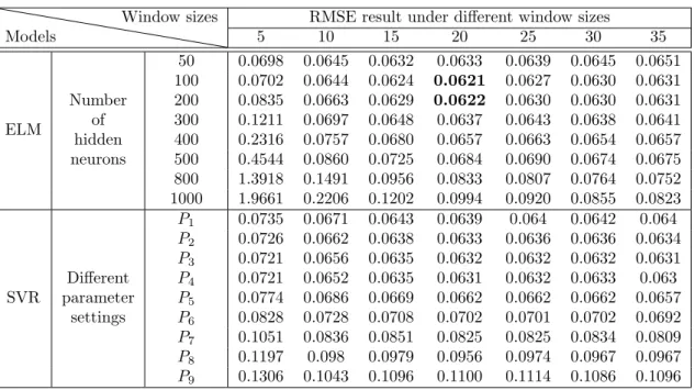
2.2 RMSE performance of ELM and SVR with different parameter settings over dif-ferent window sizes: ELM1, ...,ELM4 represent the number of hidden neurons 50, 100, 200, 300 and SVR1, ...,SVR4 show the parameter settingsP1, ..., P4 . . . 31
3.1 Illustration of the process of multivariate time series prediction . . . 38
3.2 The structures of Random Vector Functional Link Neural Network . . . 41
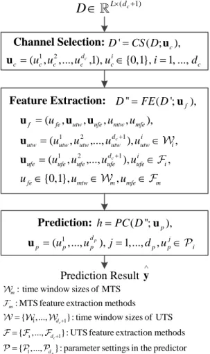
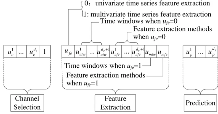
3.3 Prediction pipeline definition: given MTS D∈RL×(dc+1), the prediction result ˆy can be obtained by ˆy = f(D;uc,uf,up) after performing the operations of CS, F C and P C . . . 46
3.4 The proposed evolutionary model construction framework . . . 48
3.5 Dimension structure of the evolutionary model . . . 50
3.6 The flowchart of the proposed two-step evolutionary algorithm . . . 52
3.7 Box plot of MLP, ELM, SVR, HELM, GRUs, LSTM, iPSO, LMMLP, ADE, and the proposed EMC on All dataset . . . 61
3.8 Box plot of MLP, ELM, SVR, HELM, GRUs, LSTM, iPSO, LMMLP, ADE, and the proposed EMC on Holiday dataset . . . 61
3.9 Box plot of MLP, ELM, SVR, HELM, GRUs, LSTM, iPSO, LMMLP, ADE, and the proposed EMC on Nonholiday dataset . . . 61
3.10 Performance comparison of MLP, ELM, SVR, HELM, GRUs, LSTM, iPSO, LMMLP,
ADE, and EMC for days in one week on RMSE, MAPE and MAE . . . 62
3.11 Performance comparison of MLP, ELM, SVR, HELM, GRUs, LSTM, iPSO, LMMLP, ADE, and EMC for time stamps in one day on RMSE, MAPE and MAE . . . . 63
3.12 Performance comparison of MLP, ELM, SVR, HELM, GRUs, LSTM, iPSO, LMMLP, ADE, and EMC for different months on RMSE, MAPE and MAE . . . 63
4.1 (a) The eventually evolved PF with correlation and MSE: the population size in MOEA/D is 100 and neighborhood is 5; (b) Accumulated combination coefficients for each individual in the PF: the population size in DE is 100 . . . 81
4.2 MSE statistical summary for EMOELW, EMOELWO, ELM-PLSR, GRUs, HELM, ELM, SVR and MLP . . . 82
5.1 The training procedure of multi-resolution selective ensemble extreme learning machine . . . 87
5.2 The performance of multiple resolutions under ELM, H-ELM, -SVR and GRUs on interval and daily datasets, respectively . . . 90
5.3 The performance of MRSE-ELM on interval and daily datasets, respectively . . . 90
6.1 The problem description . . . 97
6.2 The architecture of Broad Learning System . . . 98
6.3 The illustration of the overall evolutionary ensemble learning framework . . . 103
6.4 Dimension structure of the proposed EEL . . . 104
6.5 Box plot of EELRVFL, EELELM and EELBLS with Mean, LS, PFSBS, PFSFS, NDFSBS, NDFSFS, CPF, CPFSBS and CPFSFS for Dataset A . . . 113
6.6 Box plot of EELRVFL, EELELM and EELBLS with Mean, LS, PFSBS, PFSFS, NDFSBS, NDFSFS, CPF, CPFSBS and CPFSFS for Dataset B . . . 113
6.7 Box plot of SO withps= 30,50,80,100,120,150 under RVFL, ELM and BLS for Dataset A . . . 118
6.8 Box plot of SO withps= 30,50,80,100,120,150 under RVFL, ELM and BLS for Dataset B . . . 118
6.9 Box plot of the best individual in the PF of EEL withps= 30,50,80,100,120,150 under RVFL, ELM and BLS for Dataset A . . . 118 6.10 Box plot of the best individual in the PF of EEL withps= 30,50,80,100,120,150
under RVFL, ELM and BLS for Dataset B . . . 119 6.11 Box plot of RVFL, ELM, SVR, BLS, HELM, LSTM, and the best result from
SORVFL, SOELM, SOBLS, PFRVFL, PFELM, PFBLS, EELRVFL, EELELM, EELBLS
for Dataset A . . . 120 6.12 Box plot of RVFL, ELM, SVR, BLS, HELM, LSTM, and the best result from
SORVFL, SOELM, SOBLS, PFRVFL, PFELM, PFBLS, EELRVFL, EELELM, EELBLS
2.1 The comparison of ELM and SVR with only historical electricity consumption . 32 2.2 Subset of electricity-related factors with the best prediction performance . . . 32 2.3 Subsets of environmental factors for improving prediction accuracy mostly . . . . 33 2.4 The optimal subset of all factors, respective window sizes and the number of
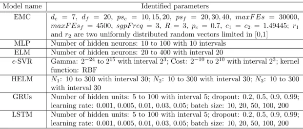
hidden neurons in ELM based on DDMS-PSO . . . 34 3.1 Identified parameters for proposed EMC and comparison models . . . 56 3.2 Performance of EMCELMand EMCRVFLon All dataset under differentpscandpsf 57 3.3 Performance of EMCELM and EMCRVFL on Holiday dataset under different psc
and psf . . . 58 3.4 Performance of EMCELM and EMCRVFL on Nonholiday dataset under different
psc and psf . . . 58 3.5 Performance comparison of EMC with the state-of-the-art models on All dataset 59 3.6 Performance comparison of EMC with the state-of-the-art models on Holiday dataset 60 3.7 Performance comparison of EMC with the state-of-the-art models on Nonholiday
dataset . . . 60 4.1 Performance comparison of EMOELWand EMOELWOunder different population
sizes in MOEA/D and DE, represented with ps1 and ps2, respectively . . . 79
4.2 Performance comparison of the proposed EMOEL under different population sizes in MOEA/D and DE (ps1 and ps2, respectively) with feature extraction . . . 80
4.3 Performance of EMOELW and EMOELWO in comparison to ELM-PLSR, GRUs,
HELM, ELM, SVR and MLP . . . 82
5.1 RMSE testing performance on interval and daily datasets . . . 91
6.1 The parameter settings in the proposed EEL . . . 109
6.2 The parameter settings in the state-of-the-art models . . . 110
6.3 Dataset A: Statistic of the individuals in different level-accumulated NDFs and the ones selected from the CPF with SBS and SFS . . . 111
6.4 Dataset B: Statistic of the individuals in different level-accumulated NDFs and the ones selected from the CPF with SBS and SFS . . . 112
6.5 Dataset A: Mean RMSE performance onps= 30,50,80,100,120,150 in MOEA/D with RVFL, ELM, and BLS under Mean, LS, PFSBS, PFSFS, NDSSBS, NDSSFS, CPF, CPFSBS and CPFSFS . . . 114
6.6 Dataset B: Mean RMSE performance onps= 30,50,80,100,120,150 in MOEA/D with RVFL, ELM, and BLS under Mean, LS, PFSBS, PFSFS, NDSSBS, NDSSFS, CPF, CPFSBS and CPFSFS . . . 115
6.7 Mean RMSE of SO and the best individuals in the PFs of EEL by employing RVFL, ELM and BLS under ps= 30,50,80,100,120,150 for Datasets A and B, respectively . . . 117 6.8 Comparison of RVFL, ELM, SVR, BLS, HELM, LSTM, SO, the best individuals
Multivariate time series (MTS) prediction plays a significant role in many practical data mining applications, such as finance, energy supply, and medical care domains. Over the years, various prediction models have been developed to obtain robust and accurate prediction. However, this is not an easy task by considering a variety of key challenges. First, not all channels (each channel represents one time series) are informative (channel selection). Considering the complexity of each selected time series, it is difficult to predefine a time window used for inputs. Second, since the selected time series may come from cross domains collected with different devices, they may require different feature extraction techniques by considering suitable parameters to extract meaningful features (feature extraction), which influences the selection and configuration of the predictor, i.e., prediction (configuration). The challenge arising from channel selection, feature extraction, and prediction (configuration) is to perform them jointly to improve prediction performance. Third, we resort to ensemble learning to solve the MTS prediction problem composed of the previously mentioned operations, where the challenge is to obtain a set of models satisfied both accurate and diversity. Each of these challenges leads to an NP-hard combinatorial optimization problem, which is impossible to be solved using the traditional methods since it is non-differentiable. Evolutionary algorithm (EA), as an efficient metaheuristic stochastic search technique, which is highly competent to solve complex combinatorial optimization problems having mixed types of decision variables, may provide an effective way to address the challenges arising from MTS prediction. The main contributions are supported by the following investigations.
First, we propose a discrete evolutionary model, which mainly focuses on seeking the in-fluential subset of channels of MTS and the optimal time windows for each of the selected
electricity consumption data with auxiliary environmental factors demonstrates the efficiency and effectiveness of the proposed method in searching for the informative time series and re-spective time windows and parameters in a predictor in comparison to the result obtained through enumeration.
Subsequently, we define the basic MTS prediction pipeline containing channel selection, fea-ture extraction, and prediction (configuration). To perform these key operations, we propose an evolutionary model construction (EMC) framework to seek the optimal subset of channels of MTS, suitable feature extraction methods and respective time windows applied to the se-lected channels, and parameter settings in the predictor simultaneously for the best prediction performance. To implement EMC, a two-step EA is proposed, where the first step EA mainly focuses on channel selection while in the second step, a specially designed EA works on fea-ture extraction and prediction (configuration). A real-world electricity data with exogenous environmental information is used and the whole dataset is split into another two datasets according to holiday and nonholiday events. The performance of EMC is demonstrated on all three datasets in comparison to hybrid models and some existing methods.
Then, based on the prediction pipeline defined previously, we propose an evolutionary multi-objective ensemble learning model (EMOEL) by employing multi-objective evolutionary algorithm (MOEA) subjected to two conflicting objectives, i.e., accuracy and model diversity. MOEA leads to a pareto front (PF) composed of non-dominated optimal solutions, where each of them represents the optimal subset of the selected channels, the selected feature extraction methods and the selected time windows, and the selected parameters in the predictor. To boost ultimate prediction accuracy, the models with respect to these optimal solutions are linearly combined with combination coefficients being optimized via a single-objective task-oriented EA. The superiority of EMOEL is identified on electricity consumption data with climate information in comparison to several state-of-the-art models.
We also propose a multi-resolution selective ensemble learning model, where multiple res-olutions are constructed from the minimal granularity using statistics. At the current time stamp, the preceding time series data is sampled at different time intervals (i.e., resolutions) to
eters are first trained. Feature selection technique is applied to search for the optimal set of trained base learners and least square regression is used to combine them. The performance of the proposed ensemble model is verified on the electricity consumption data for the next-step and next-day prediction.
Finally, based on EMOEL and multi-resolution, instead of only combining the models generated from each PF, we propose an evolutionary ensemble learning (EEL) framework, where multiple PFs are aggregated to produce a composite PF (CPF) after removing the same solutions in PFs and being sorted into different levels of non-dominated fronts (NDFs). Feature selection techniques are applied to exploit the optimal subset of models in level-accumulated NDF and least square is used to combine the selected models. The performance of EEL that chooses three different predictors as base learners is evaluated by the comprehensive analysis of the parameter sensitivity. The superiority of EEL is demonstrated in comparison to the best result from single-objective EA and the best individual from the PF, and several state-of-the-art models across electricity consumption and air quality datasets, both of which use the environmental factors from other domains as the auxiliary factors.
In summary, this thesis provides studies on how to build efficient and effective models for MTS prediction. The built frameworks investigate the influential factors, consider the pipeline composed of channel selection, feature extraction, and prediction (configuration) si-multaneously, and keep good generalization and accuracy across different applications. The proposed algorithms to implement the frameworks use techniques from evolutionary computa-tion (single-objective EA and MOEA), machine learning and data mining areas. We believe that this research provides a significant step towards constructing robust and accurate models for solving MTS prediction problems. In addition, with the case study on electricity consump-tion predicconsump-tion, it will contribute to helping decision-makers in determining the trend of future energy consumption for scheduling and planning of the operations of the energy supply system.
Introduction
Time series prediction is an important research topic and has attracted a considerable amount of attention in the past decades [Brockwell et al., 2002, De Gooijer and Hyndman, 2006, Montgomery et al.,1990,Weigend,2018,Zhang,2003]. It refers to the process of predicting a future value or values by analyzing the trend of past and current ones [Hamilton,1994,Paaßen et al., 2018, Weigend, 2018]. The increasing use and availability of intelligent devices and data storage provide an efficient way to collect time series data composed of multiple variables (i.e., multivariate time series; MTS) [Cao et al., 1998, Chakraborty et al., 1992, Che et al., 2018,Wang and Han,2015] derived from complex systems using a variety of different sources [Alahakoon and Yu,2016,Barker et al.,2012,Chaouch,2014,Stisen et al.,2015], where each individual time series (i.e., univariate time series; UTS) indicates the data collected from a certain data source (so-called channel). In this regard, MTS prediction has tackled real-world problems in many practical data mining domains, such as finance [Sun et al., 2015], energy consumption [Fan et al., 2014, Jahandari et al., 2018], medical care [Li-wei et al., 2015] and climate studies [Cadenas et al.,2016,Xu et al.,2018] since it contains more useful information expected than in the UTS.
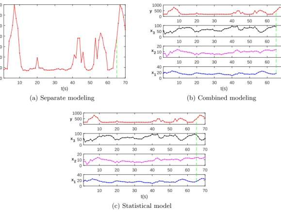
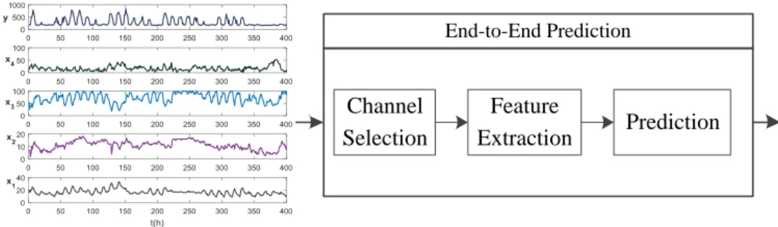
The modeling of MTS prediction is classified into three categories [Chakraborty et al.,1992, Han and Xu,2018, Kattan et al.,2015], includingseparate modeling,combined modeling, and statistical model. Given multivariate dataset (x1,x2,x3,y), y represents energy consumption
data to be predicted and (x1,x2,x3) are exogenous factors, i.e., temperature, wind speed and
dew point, which are supposed to influence the behavior of y. For separate modeling, each UTS is analyzed without utilizing the interdependencies related to auxiliary time series, such as the example illustrated in Fig. 1.1a, where only the historical trend is assumed to influence the future behavior ofy. Instead of treating each time series individually,combined modeling [Adhikari,2015,Chandra,2015,Sun et al.,2017,Wu and Lee,2015,Yazdanbakhsh and Dick, 2017] uses the past data of all variables within a time window, such as Fig. 1.1b, the predicted values of y can be obtained via using the information fromx1,x2,x3,y before the green line.
Statistical model [Voronin and Partanen, 2014] is another modeling presented in Fig. 1.1c, where multiple learning tasks, i.e., the future values of each of x1,x2,x3,y, are predicted
simultaneously by exploiting commonalities and differences across tasks.
t(s) 10 20 30 40 50 60 70 y 100 200 300 400 500 600 700 800
(a) Separate modeling
10 20 30 40 50 60 70 y 0 500 1000 10 20 30 40 50 60 70 x3 0 50 100 10 20 30 40 50 60 70 x2 0 10 20 t(s) 10 20 30 40 50 60 70 x1 0 20 40 (b) Combined modeling 10 20 30 40 50 60 70 y 0 500 1000 10 20 30 40 50 60 70 x3 0 50 100 10 20 30 40 50 60 70 x2 0 10 20 t(s) 10 20 30 40 50 60 70 x1 0 20 40 (c) Statistical model
Figure 1.1: Illustrations of three different MTS prediction models
Most of the existing studies mainly focus on combined modeling since separate modeling may not have sufficient knowledge of the underlying data for obtaining the desirable prediction
performance. Interdependencies among MTS have been modeled usingstatistical method, such as autoregressive integrated moving average (ARIMA) [Voronin and Partanen, 2014, Zhang, 2003], which provides insight into the dynamic relationship of the time series and often produces prediction superior to independent univariate models (i.e.,separate modeling). Statistical model mainly concentrates on obtaining the satisfied accuracy accumulated by all targeted variables, such as the example depicted in Fig. 1.1c, where the performance of a specific prediction task, i.e.,y, may be sacrificed. Additionally, computational intelligence methods have risen as an alternative to classical statistical models, offering competitive performance in multivariate prediction [Cadenas et al., 2016]. In this dissertation, we mainly target at MTS prediction using combined modeling for a certain task.
Since not all channels are informative for the modeling, it is essential to remove the ir-relevant and redundant variables [Chen and Lee, 2015, Crone and Kourentzes, 2010] using feature selection methodologies [Crone and Kourentzes,2010,Hu et al.,2015,Koprinska et al., 2015] for robust and accurate prediction. Feature extraction is fundamentally important for improving prediction performance by learning the valuable features embedded in the time se-ries [Bianchi et al.,2015, Fan et al.,2014, Luo et al.,2015], where the extracted features are reconstructed as a vector for inputs. Ensemble learning, which uses multiple algorithms to obtain better predictive performance than that could be obtained from any of the constituent learning algorithms alone, has been studied widely in time series prediction tasks [Adhikari, 2015,Adhikari and Agrawal,2012,Donate et al.,2013,Krawczyk et al.,2017,Li et al.,2016a]. With the development of the evolutionary computation [Chugh et al.,2018,Storn and Price, 1997,Zhang et al., 2018b], its advantage in handling large-scale, non-differentiable and com-plex problems without any information about optimized problems for its global convergence ability and strong robustness, has been found. Recently, many optimization algorithms such as particle swarm optimization (PSO) [Eberhart and Kennedy,1995], differential algorithm (DE) [Kazimipour et al.,2014,Qin and Li,2013,Storn and Price,1997] etc., have been successfully applied to feature selection [Jain et al., 2018, Xue et al., 2016], predictor architecture opti-mization [Hu et al.,2014, Liang et al., 2014] and ensemble learning [Chandra and Yao,2006, Fernandez Navarro et al.,2013,Smith and Jin,2014,Zhang et al.,2018a,2017b].
In this thesis, we mainly investigate the research gaps in MTS prediction on methods to exploit informative factors (channel selection), address the combinatorial optimization prob-lem composed of channel selection, feature extraction in relation to the explored factors and model configuration synchronously, and construct effective ensemble learning model using com-putational intelligence involving evolutionary computation, machine learning and data mining methodologies. Based on the formulated research questions, the contributions verify the rea-sons why modeling evolutionary MTS prediction is worth being studied.
1.1
Motivations
MTS prediction has been widely applied to a variety of areas, such as international tourism demand [Du Preez and Witt,2003], hourly urban water demand [Herrera et al., 2010], stock price prediction [Lin et al., 2009] and load forecasting [Hippert et al., 2001]. Since the irrel-evant or redundant information may decrease the accuracy, it is fundamentally important to investigate the main factors that can contribute to improving prediction performance mostly, where time windows for each influential factors need to be identified for inputs by selecting a suitable predictor and its parameters. This is a difficult task since the combination possibilities increase exponentially when the number of time series increases. Accordingly, a general model is required to analyze the factors and the time windows for each informative factor as well as the parameters in the predictor.
The time series from cross domains may require different feature extraction techniques and time windows because they perform variably on their time trends. For each selected channel, allocating suitable feature extraction techniques and time windows to be selected is of vital importance to boost predictive accuracy. With different subsets of feature extraction techniques and time windows, the lengths of the inputs (i.e., features) obtained from all selected channels fed to the predictor differ, and accordingly, it is difficult to predefine the architecture and select suitable parameters of the predictor for a specific prediction task. Predictor selection and configuration are also necessary. The problem corresponding to reconciling channel selection, feature extraction, and prediction (configuration) jointly is deserved to be studied.
model configuration, the optimal solution exploited through a hypothesis space leads to good prediction for a particular problem. However, the performance of a data-driven model could be influenced by various factors [Hu et al.,2012], e.g., capricious environmental uncertainties, considerable variability in the operation condition of different system units, varying linear or nonlinear degradation patterns, the available number of sensors to monitors the system and the number of data samples [Zhang et al.,2017b]. Therefore, a single model, after optimally configured based on the data collected under a specific situation, may not have the desirable performance for the prediction problems from other domains. Ensemble learning, combining a variety of models, may provide an effective and alternative way to address MTS prediction problems given its superiority over generalization and accuracy across different applications in comparison to single model [Barber and Bishop,1998,Sollich and Krogh,1996,Zhou,2015].
1.2
Research Challenges
Given the number of auxiliary time series n in addition to the predicted time series for an MTS prediction task, the state for each time series is binary (i.e., 1 and 0 represent ’selected’ and ’not selected’). If there are t different time windows to be selected for each channel, the total combinations will be 2ntn+1. To exploit the informative factors and the respective time windows is to find the optimal solution among these 2ntn+1 combinations. It is impossible to solve this non-differentiable problem with enumeration given its extremely time-consuming process.
Based on the exploration of the informative channels, it is important to allocate effec-tive feature extraction methods for each selected channel of MTS. The extracted features are reconstructed as a vector fed to the task-oriented model by suitable predictor selection and configuration [Hu et al.,2014]. The challenge arising from channel selection, feature extraction, and prediction (configuration) is how to perform them together and adaptively fine-tune the rest when one of the settings is changed. However, the selection among these operations having numerous combination possibilities leads to an NP-hard problem, which is non-differentiable and fundamentally difficult to be formulated mathematically, and accordingly, it is impossible to address it with gradient descent, a typical approach to find an optimal configuration in a
search space.
Given the typical pipeline composed of channel selection, feature extraction, and prediction (configuration), each part is related to a combinatorial optimization problem. Most existing works in this regard have targeted at a specific part in the pipeline without addressing all three parts as a whole. A widely approved fact is that ensemble learning [Adhikari, 2015, Adhikari and Agrawal, 2012, Chandra and Yao, 2006, Donate et al., 2013, Krawczyk et al., 2017,Li et al., 2016a,Sun et al.,2018] combining different models has been demonstrated to have better generalization and performance than each of its constituents, where the challenge is how to generate useful individuals to be combined with the effective combination rule and the individuals should be as more accurate as possible and as more diverse as possible.
The key challenges arising from MTS prediction are established as follows:
• Investigating the informative channels of MTS and respective time windows that can contribute the most to the prediction performance
• Performing channel selection, feature extraction, and prediction (configuration) simulta-neously
• Building the efficient model that can target at the MTS prediction problems consisted of channel selection, feature extraction, and prediction (configuration) jointly
• Generating useful members satisfied high accuracy and model diversity among them for ensemble learning
• Designing effective combination rules to combine the generated members for the best ensemble.
1.3
Research Questions
To overcome the aforementioned challenges, the following research questions (RQs) are defined to provide an overarching view on what this thesis is tailored for.
RQ-1. How to explore the influential factors and respective time windows for multivariate time series prediction?
For the prediction task with various auxiliary time series, it is necessary to investigate whether they can help to improve prediction accuracy and identify the one that can contribute the most to accurate prediction. In addition, different time series may require different time windows. For this research question, we mainly concentrate on building a model to explore the optimal subset of channels of MTS and respective time windows as well as the suitable predictor that can lead to the highest prediction accuracy.
RQ-2. How to construct an evolutionary model for multivariate time series prediction
com-posed of channel selection, feature extraction, and prediction jointly?
Considering the heterogeneity of time series from cross domains, they may require different feature extraction methodologies to discover the valuable patterns embedded in the raw data, which leads to predictor selection and configuration since most existing predictors need to be well configured given the data collected under a certain situation. Based on the analysis of RQ-1, we mainly focus on constructing the model that can process the core operations composed of channel selection, feature extraction, and prediction (configuration) simultaneously.
RQ-3. How to construct a multi-objective ensemble learning framework for multivariate time
series prediction composed of channel selection, feature extraction, and prediction jointly?
Considering the effectiveness of ensemble learning, instead of choosing one optimal solu-tion for the MTS predicsolu-tion pipeline defined inRQ-2, multi-objective evolutionary algorithm (MOEA) is applied to search for the optimal parameters of the model as well as the optimal features fed to the model subjected to two conflicting criteria, i.e., accuracy and diversity. The trained models corresponding to the optimal solutions in the pareto front (PF) that is gener-ated from MOEA are linearly combined with combination coefficients being optimized via a single-objective EA to obtain the accurate prediction.
RQ-4. How to perform ensemble learning via constructing multiple resolutions for time series prediction?
Since time series at different granularities/frequencies may capture more information for predicting the future trend, we propose a new mechanism to construct multiple resolutions based on the raw time series with minimal granularity. Multiple base learners with different parameter settings over each resolution are first trained. Feature selection technique is applied to seek the optimal subset of trained base learners and least square (LS) is used to combined the selected models.
RQ-5. How to build an evolutionary ensemble learning framework for multivariate time series
prediction composed of channel selection, feature extraction, and prediction jointly?
RQ-5 is an extension ofRQ-3 and RQ-4. Instead of exploiting the best ensemble per-formance across each PF like RQ-3, we mainly concentrate on building the framework that aggregates multiple PFs produced by different population sizes to generate different levels of non-dominant fronts (NDFs). The ensemble learning is performed on the level-accumulated NDF using feature selection techniques and the selected models are linearly combined by LS.
1.4
Research Contributions
By addressing the aforementioned RQs, the contributions of this thesis are summarized as follows:
1. Informative factor analysis
– We define the additional elements, i.e., time windows and the parameter settings in the predictor, to be exploited as well as the informative factors in MTS prediction for obtain-ing the highest prediction accuracy. To solve this problem efficiently and effectively, we propose a discrete dynamic multi-swarm PSO (DDMS-PSO) to investigate the informa-tive factors and respecinforma-tive time windows along with the suitable predictor configuration for the best prediction performance. DDMS-PSO is not only limited to the case study of electricity consumption prediction with auxiliary factors but also provides a solution for MTS prediction in general.
2. Evolutionary model construction
– We define the typical MTS prediction pipeline consisted of channel selection, feature extraction, and prediction (configuration). To address the combinatorial optimization problems in each operation synchronously, we propose an end-to-end framework, called evolutionary model construction (EMC) to seek the optimal solution. The proposed EMC framework can work with any predictor by removing the unnecessary parts in the pipeline, it contributes to different application domains in MTS prediction. The proposed two-step EA can be dynamically adjusted to implement EMC.
3. Evolutionary multi-objective ensemble learning
– We propose an evolutionary multi-objective ensemble learning (EMOEL) framework to address MTS prediction problem composed of channel selection, feature extraction and prediction (configuration) in parallel. Instead of only choosing one optimal solution, EMOEL employs MOEA to generate a set of non-dominant optimal solutions in the PF subjected to prediction accuracy and model diversity. EMOEL can contribute to relieve labour-intensive model tuning and produce better prediction performance than each of its constituents by linearly combining the eventually evolved solutions.
4. Multi-resolution construction
– We propose a mechanism to construct multiple resolutions (MRs) to capture more infor-mation from the raw time series for ensemble learning, where each resolution is trained across extreme learning machine (ELM) by considering different numbers of hidden neu-rons. The optimal subset of the trained models is selected by sequential forward selection (SFS) and combined with LS. The proposed multi-resolution selective ensemble is not limited in being applied with ELM and SFS.
5. Evolutionary ensemble learning
– We propose an evolutionary ensemble learning (EEL) framework to solve the MTS pre-diction problems consisted of channel selection, feature extraction and prepre-diction
(con-figuration). Different with ELOEL proposed in RQ-3, where the ensemble learning is performed on each PF, multiple PFs produced by different population sizes in EEL are merged to generate a composite PF (CPF) that contains different levels of non-dominated fronts (NDFs). SFS and sequential backward selection (SBS) are chosen to select the optimal subset of models in the level-accumulated NDF and LS is used to combined the selected models. EEL provides another solution for facilitating MTS prediction by preserving good solutions in other PFs. The implementation of EEL can be replaced by other methodologies that have the same problem-solving ability.
1.5
Case Studies and Datasets
In this dissertation, two real-world MTS datasets, i.e., electricity consumption and air quality datasets, are applied to verify the effectiveness of the proposed frameworks and algorithms that are designed to solve the formulated research questions on MTS prediction. Each of the studied datasets has multivariate data from cross domains. Electricity consumption data includes historical electricity consumption1, electricity-related factors1 and environmental
fac-tors2, which is collected through the RMIT Sustainable Urban Precincts Program (SUPP) project3. Air quality data that includes date information, environmental factors, and location, is one benchmark PM2.5 Data of Five Chinese Cities Data Set from the UCI repository4. Elec-tricity consumption data from RMIT University is used in Chapter 2, 3, 4 and 5. The building studied in this thesis is a mixed use with 13 floors and total gross area more than 17000m2. It contains staff offices, teaching spaces, lectures, public activities, meeting rooms, kitchen rooms, and coffee shops. The activities in this building range all the year round based on academic calendar, public events, and peak and off-peak period around the academic calendar as well as daily peak and off-peak patterns. Both electricity consumption and air quality datasets are applied to the problem observed in Chapter 6. The details of the dataset description are depicted in each chapter.
1https://www.utiliview.com.au/login.aspx 2 http://www.wunderground.com 3 https://www.rmit.edu.au/about/our-values/sustainability/sustainable-urban-precincts-program 4 https://archive.ics.uci.edu/ml/datasets/PM2.5+Data+of+Five+Chinese+Cities
1.6
Thesis Organization
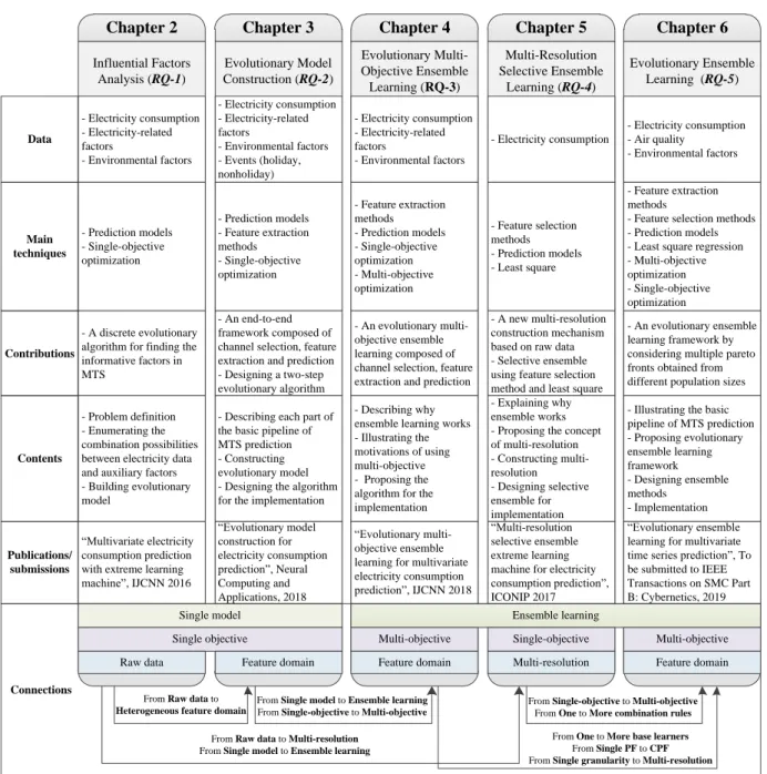
This chapter mainly introduces some background, the motivations, the challenges, and con-tributions behind MTS prediction. The rest of the thesis is structured as follows. Since the literature review (i.e., related work) is included in each main chapter, we do not have a specific chapter for that. In Chapter 2, a single-objective discrete optimization algorithm is proposed for finding the optimal subset of channels of MTS and respective time windows for the best prediction performance to explore informative factors for a specific MTS prediction task. Based on the analysis of Chapter 2 over raw data, Chapter 3 constructs an evolutionary framework, where an evolutionary algorithm is proposed to target at MTS prediction task composed of channel selection, feature extraction, and prediction (configuration) simultaneously. In Chap-ter 4, for the pipeline in ChapChap-ter 3, we propose an ensemble learning framework based on multi-objective optimization, where MOEA is employed to seek a set of optimal solutions sub-jected to prediction accuracy and model complexity. The trained models corresponding to the optimal solutions are linearly combined by a single-objective EA. Chapter 5 is based on the time series from one domain, where multiple resolutions are constructed and trained with the base learners. A new selective ensemble method is proposed to combine the selected models. Chapter 6 is an extended work based on Chapter 4 and Chapter 5, where a new evolution-ary ensemble learning framework is proposed by aggregating multiple PFs to generate NDFs and various ensemble mechanisms are designed. The main contributions and connections from Chapter 2 to Chapter 6 are detailed in Fig. 1.2. In Chapter 7, we summarize the main contributions, key findings and the limitations of the proposed methods. Subsequently, the significance of this research and the potential future works are also discussed.
Chapter 2 Influential Factors Analysis (RQ-1) Chapter 3 Evolutionary Model Construction (RQ-2) Chapter 4 Evolutionary Multi-Objective Ensemble Learning (RQ-3) Chapter 5 Multi-Resolution Selective Ensemble Learning (RQ-4) Chapter 6 Evolutionary Ensemble Learning (RQ-5) - Electricity consumption - Electricity-related factors - Environmental factors Data - Electricity consumption - Air quality - Environmental factors - Electricity consumption - Electricity-related factors - Environmental factors - Events (holiday, nonholiday) - Electricity consumption - Electricity-related factors - Environmental factors - Electricity consumption - Prediction models - Single-objective optimization Main techniques - Prediction models - Feature extraction methods - Single-objective optimization - Feature extraction methods
- Feature selection methods - Prediction models - Least square regression - Multi-objective optimization - Single-objective optimization - Feature selection methods - Prediction models - Least square - Feature extraction methods - Prediction models - Single-objective optimization - Multi-objective optimization - A discrete evolutionary algorithm for finding the informative factors in MTS
Contributions
- An end-to-end framework composed of channel selection, feature extraction and prediction - Designing a two-step evolutionary algorithm
- An evolutionary multi-objective ensemble learning composed of channel selection, feature extraction and prediction
- A new multi-resolution construction mechanism based on raw data - Selective ensemble using feature selection method and least square
- An evolutionary ensemble learning framework by considering multiple pareto fronts obtained from different population sizes
- Describing each part of the basic pipeline of MTS prediction - Constructing evolutionary model - Designing the algorithm for the implementation
From Raw data to Heterogeneous feature domain
From Single model to Ensemble learning From Single-objective to Multi-objective
From Raw data to Multi-resolution From Single model to Ensemble learning
From One to More base learners From Single PF to CPF From Single granularity to Multi-resolution From Single-objective to Multi-objective
From One to More combination rules
- Problem definition - Enumerating the combination possibilities between electricity data and auxiliary factors - Building evolutionary model
Contents
- Describing why ensemble learning works - Illustrating the motivations of using multi-objective - Proposing the algorithm for the implementation
- Explaining why ensemble works - Proposing the concept of multi-resolution - Constructing multi-resolution - Designing selective ensemble for implementation
- Illustrating the basic pipeline of MTS prediction - Proposing evolutionary ensemble learning framework - Designing ensemble methods - Implementation Publications/ submissions “Multivariate electricity consumption prediction with extreme learning machine”, IJCNN 2016 “Evolutionary model construction for electricity consumption prediction”, Neural Computing and Applications, 2018 “Evolutionary multi-objective ensemble learning for multivariate electricity consumption prediction”, IJCNN 2018
“Multi-resolution selective ensemble extreme learning machine for electricity consumption prediction”, ICONIP 2017
“Evolutionary ensemble learning for multivariate time series prediction”, To be submitted to IEEE Transactions on SMC Part B: Cybernetics, 2019 Connections Single model Single objective Ensemble learning Multi-objective Single-objective Multi-objective
Raw data Feature domain Feature domain Multi-resolution Feature domain
Influential Factors Analysis
Nowadays the ever-increasing energy consumption in buildings has caused supply shortages and adverse environmental impacts. The accurate prediction of energy consumption in smart buildings may help to monitor and control energy usage. As energy consumption is inevitably affected by exogenous factors such as temperature, wind speed etc., it is fundamentally impor-tant to select the factors that can help improve the prediction accuracy, where it is essential to select the suitable time windows and predictor. ELM is demonstrated to be a powerful tool for electricity consumption prediction based on its competitive prediction accuracy and supe-rior computational speed compared to support vector machine/regression (SVM/R). Moreover, ELM is utilized to investigate the potentials of using auxiliary information such as electricity-related factors and environmental factors to augment the prediction accuracy obtained by purely using the electricity consumption factors. Furthermore, we formulate a combinatorial optimization problem of seeking an optimal subset of auxiliary factors and their corresponding optimal window sizes using the most suitable ELM structure, and propose a discrete dynamic multi-swarm particle swarm optimization (DDMS-PSO) to address this problem. Experimen-tal studies on a real-world building dataset demonstrate that electricity-related factors improve accuracy while environmental factors further boost accuracy. By using DDMS-PSO, we find a subset of electricity-related and environmental factors, their respective window sizes, and the number of hidden neurons in ELM which leads to the best prediction accuracy.
2.1
Introduction
The rapidly growing world energy usage has caused issues of supply difficulties, exhaustion of energy resources and heavy environmental impact. Electricity consumption as a form of energy consumption, with the expansion of residential and commercial areas, has grown, which is a threat to sustainable development. The prediction of electricity consumption in buildings does not only help to improve energy monitoring and usage in buildings but plays a vital role in improving the electrical performance, with the aim of achieving energy consumption conservation and reducing the environmental impact [Foucquier et al.,2013]. Also, electricity consumption prediction plays a significant role in decision-making and future planning that rely on prediction accuracy.
Electricity consumption prediction has a history of more than 20 years. It has been a way to measure the characteristics of buildings and aid the development of electric power plants, therefore electricity prediction has been an application of time series analysis [Zhao and Magoul`es,2012]. It is an indispensable part of managing and researching power systems, and it can make full use of electricity and ease the conflict between supply and demand based on the analysis of the existing electric energy [Yalcintas and Akkurt,2005]. Electricity consumption is highly dependent on electric power, economic, social and meteorological factors. The precision of prediction is very important for informing the analyses of electric power exchange, trading evaluation, network function, security and trends, and the safety strategy of reduction load.
Existing electricity consumption prediction research always involves multi-variate historical data. Different researchers use different attributes to analyze this issue. Thermal comfort is a criterion to evaluate the environment and can be regarded as a factor which will affect electricity usage [Roetzel and Tsangrassoulis,2012]. Moreover, some other factors such as temperature, events, wind speed or features in the buildings are always taken into consideration for improving the prediction accuracy. The area of windows, walls, partitions and floors, the type of windows and walls are regarded as factors which have a direct or indirect relationship with electricity consumption [Kalogirou et al., 1997]. Temperatures, space heating demand, water heating demand, and energy demand are applied to help improve the performance of prediction in [Olofsson et al.,1998].
We aim to predict electricity usage of a university building. ELM [Chen et al.,2012,Wan et al., 2014, Wang and Han, 2014b, Yang et al., 2018, 2017, Zeng et al., 2017] is used for electricity consumption prediction through exploring the predictive performance of historical electricity consumption logs along with electricity-related and environmental data. Further-more, a DDMS-PSO is proposed to address the optimization problem of discrete values in order to find a subset of all factors, regardless of the heterogeneity of their feature space, with their respective window sizes and the number of hidden neurons which can lead to the best prediction performance.
The dataset is collected from the smart meters of the buildings in the city campus of RMIT University, Melbourne. We mainly focus on understanding the trend of electricity consumption under the influence of electricity-related and environmental factors on energy usage. Auxiliary environmental data is crawled from an online weather station that broadcasts periodic readings from every 20-minutes to 1-hour. The output of prediction is useful to help event planning and resource management. The following aspects are explored in this chapter.
• Historical smart meter data is used to evaluate and forecast the buildings’ future electric-ity consumption. Then the result is regarded as the baseline to evaluate if the auxiliary information can help improve the prediction accuracy.
• Electricity-related factors are added to identify if they have an effect on improving the prediction performance and which factors can increase the accuracy the most.
• Based on the best combination of the electricity-related factors, explore if environmental factors actually influence the prediction accuracy and the optimal subset of the environ-mental factors.
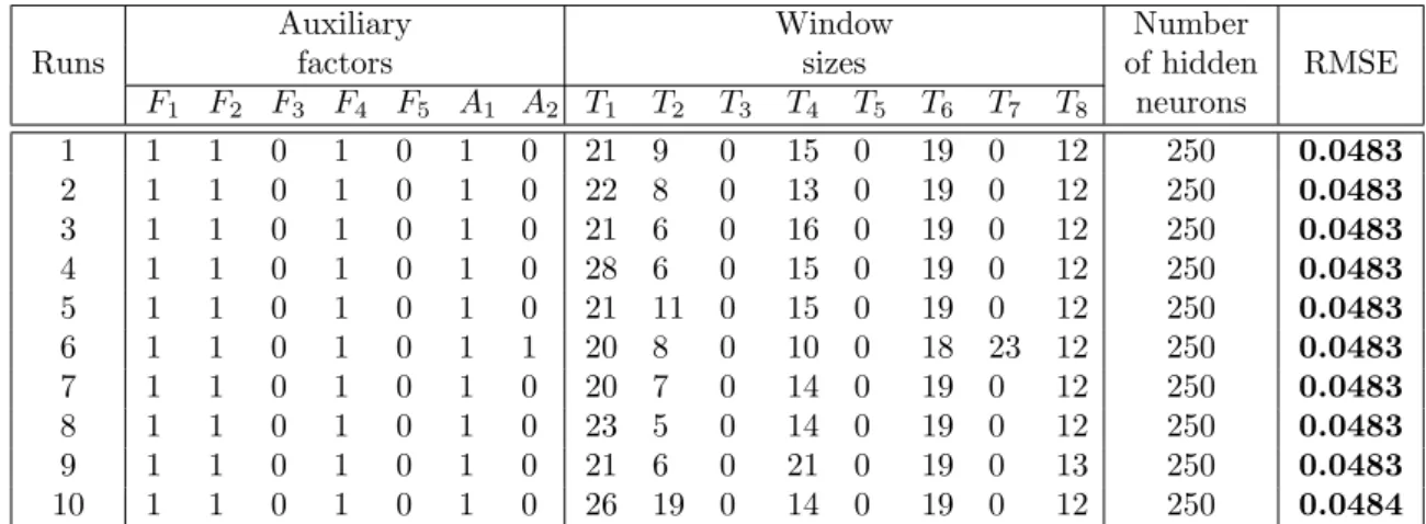
• Evolutionary algorithm is applied to explore if there is a subset of electricity-related and environmental factors, their respective window sizes and a suitable number of hidden neurons in ELM to generate the best prediction accuracy.
In the next section, we present the related work on electricity consumption prediction. Problem definition is depicted in Section 2.3. The proposed solutions to address the problems
are introduced in Section 2.4. Section 2.5 mainly focuses on experimental settings and related results. Conclusions are given in Section 2.6.
2.2
Related Work
2.2.1 Electricity Consumption Prediction
Many methodologies have been employed for electricity consumption prediction, which includes artificial neural networks (ANNs) [Park et al.,1991], fuzzy inference system (FIS) [Ying and Pan,2008] and SVM [Kavaklioglu,2011]. Moreover, Zhao and Magoul`es[2012] categorize the methodologies into five different kinds based on the reviewed paper: engineering methods, statistical methods, ANN, SVM [Dong et al., 2005] and Grey Models. Foucquier et al. [2013] summarize the state-of-the-art methods as statistical methods which include multiple linear regression or conditional analysis, ANN and SVM as well as some hybrid models which combine two or three of the above methods. Among all the methodologies, ANN and SVR are widely used in electricity consumption [Tso and Yau,2007]. However, it is very difficult to say which one outperforms others without complete comparison under the same circumstances because each of them is still being developed [Zhao and Magoul`es,2012].
2.2.2 ELM and Its Applications
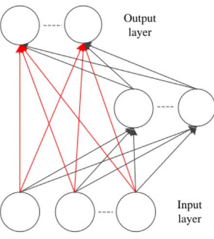
A new learning method which was proposed by Huang et al.[2006], ELM, mainly focuses on solving the drawbacks caused by gradient descent based algorithms such as back propagation (BP). ELM is based on single hidden layer feedforward neural network architecture and includes three different layers, input layer, hidden layer, and output layer, shown as Fig. 2.1. The hidden bias and the weight for connecting the input layer and hidden layer are generated randomly and maintained through the whole training process.
Assuming dataset (xi,yi) with a set ofM distinct samples, satisfiedxi ∈ Rd1 andyi ∈ Rd2, a SLFN with N hidden neurons can be mathematically formulated as:
N X i=1
Input layer Hidden layer Output layer
Figure 2.1: The structures of Extreme Learning Machine
wheref is the activation function;wi represents the weights for connecting the input layer and hidden layer; bi is bias andβi is the output weight.
In ELM, the structure perfectly approximates to the given output data: N
X i=1
βif(wTi xj+bi) =yj,1≤j≤M (2.2) Which can be written as HB=Y, the matrixH can be represented as:
H= f(wT1x1+b1) · · · f(wTNx1+bN) · · · · f(wT1xM +b1) · · · f(wTNxM +bN) (2.3) B= (βT1,βT2, ...,βTN)T and Y= (yT 1,yT2, ...,yTM)T.
The output weight B is calculated by B=H+Y, andH+ is a Moore-Penrose generalized inverse of H [Rao and Mitra,1971]. Theoretical proofs and a more thorough presentation of the ELM algorithm are detailed in the original paper [Huang et al.,2006].
ELM does not have so many parameters to be adjusted except for the number of hidden neurons, which makes it easier to be applied in regression [Li et al., 2015b, Sajjadi et al., 2016, Wan et al., 2014, Zhang et al., 2012] or classification [Huang et al., 2010] issues and very low computational cost during the process of training. Recently, ELM has been gradually gained much attention for its application in time series prediction, such as predicting sales
in fashion retailing in [Sun et al., 2008]. ELM is utilized for electricity price forecasting and has demonstrated its fast computational ability [Chen et al., 2012]. ELM is used for wind power density prediction in [Mohammadi et al.,2015b] and is compared with ANN and SVM. Mohammadi et al.[2015a] apply ELM successfully to daily dew point temperature prediction. The works related to the application of ELM in time series domain are not limited as mentioned, more examples such as [Chen et al.,2012,Wan et al.,2014,Wang and Han,2014b,Yang et al., 2018,2017,Zeng et al.,2017].
2.2.3 Evolutionary Algorithms for Energy Consumption Prediction
EA [Liang et al.,2006a] is being widely used to handle large-scale, non-differentiable and com-plex multi-mode problem without any information about optimized problems for its global convergence ability and strong robustness. Many optimization algorithms have been success-fully applied in time series prediction. PSO is used to optimize the input subset for SVM in time series prediction [Zhang and Hu, 2005]. Shafie-Khah et al. [2011] utilize PSO to opti-mize RBFN for obtaining a robustness prediction structure for price forecasting of electricity markets. Azadeh et al. [2007] use GA to tune all parameters for NN applied in predicting electrical energy consumption. Almost all methods such as GA, PSO, ant colony optimization (ACO), DE applied to renewable and sustainable energy are reviewed in [Banos et al., 2011]. Therefore, the optimization methodologies are popular for solving parameters adjustment in energy consumption prediction.
2.3
Problem Definition
2.3.1 Scenario Assumption
Assuming T which represents the length of time series, is expressed as T = {t1, t2, ..., tq}, q means the number of sample points, therefore our related time series dataset includes 3 aspects:
• Electricity-related factors rT, defined as rT ={rT1, r2T, ..., rnT}, where n is the number of the internal factors.
• Environmental factors zT, defined as zT = {zT1, z2T, ..., zTm}, where m is the number of environmental time series, including temperature, dew point(a measure of atmospheric moisture), humidity(the amount of water vapor in the air), wind speed(caused by air moving from high pressure to low pressure, usually due to changes in temperature), sea level(offer insights into ongoing climate change) etc.
2.3.2 Problem Definition
In time series prediction, there are one-step-ahead prediction and multi-step-ahead prediction. One-step-ahead prediction mainly focuses on the next single value ahead while multi-step-ahead prediction takes multiple future values into consideration. As it is known that multi-step-ahead prediction is much more complex because of the accumulation of errors and increasing uncertainties, we are focusing on exploring an optimal subset of auxiliary factors for the best prediction accuracy, so in order to decrease the influence of other uncertainties for this problem, we only focus on one-step-ahead time series prediction.
We have three different types of dataset, electricity consumption xT, electricity-related factors rT, rT ⊂ Rn, environmental factors zT, zT ⊂ Rm. To explore the influence of all these factors, two general subproblems which should be solved are defined as follows:
• Explore if electricity-related factors and environmental factors improve prediction accu-racy.
• Explore if there is an optimal subset of all auxiliary factors, their respective window sizes, and the number of hidden neurons in ELM which can obtain the best prediction performance.
2.4
Proposed Solutions
2.4.1 An Approach for Solving The First Subproblem
ELM has been proven to be capable of universal approximation in a satisfied sense, and it has been shown to have good generalization capabilities and extremely fast speed [Huang et al., 2010]. The only task for applications is to select a suitable activation function and set the number of hidden neurons. Moreover, in comparison to conventional learning approaches, it avoids many difficulties such as learning rates, learning epochs, stop criteria and local optima [Zhang et al.,2012]. All the advantages are motivations for us to utilize it as a basic prediction model for electricity consumption prediction.
There are two different kinds of factors to be taken into consideration as well as historical electricity data. To solve the first problem, the factors are added gradually with several different predefined window sizes, three steps for addressing the first subproblem are defined as follows: • Only use the historical electricity consumption to perform prediction in order to further
identify if other factors have an effect on improving prediction performance.
With the aim of finding out which factors will improve the prediction accuracy, a baseline is necessary for further comparison. All prediction results that are generated with differ-ent combinations of factors must be compared with the result of only historical electricity consumption.
AssumingH ={H1, H2, ..., HD}, d= 1,2, ..., Dis the set of different time series, we have:
xt+1=f(xt, xt−1, ..., xt−Hd−1) (2.4)
whereHd is the length of dth time window used for prediction andf() is the prediction function of a certain predictor.
• Find which factors influence the prediction accuracy the most among all electricity-related factors.
The electricity-related factors are added to the historical electricity consumption dataset to explore their single and overall performances with the predefined window sizes. The performance is compared with the result of purely electricity consumption.
xt+1 =f(xt, xt−1, ..., xt−Hd−1;r
i
t, rit−1, ..., rit−Hd−1), i= 1,2, ..., m (2.5)
• Among the environmental factors, find which of them help to improve the prediction accuracy for this problem with the influence of electricity-related factors.
Based on the electricity-related factors, a further exploration of the optimal combination of environmental factors is necessary.
xt+1=f(xt, xt−1, ..., xt−Hd−1;r c t, rct−1, ..., rct−Hd−1;z j t, z j t−1, ..., z j t−Hd−1), j = 1,2, ..., n (2.6) where c represents the electricity-related factors that have an effect on improving the prediction accuracy.
The first subproblem is addressed by investigating the potential influence of electricity-related factors and environmental factors step by step, which means that the next step is always based on the previously selected factors until an optimal subset of all auxiliary factors is found. With a larger set of factors, there are many different combinations, which will cause high computational cost, accordingly, a new approach is necessary to address the second subproblem.
2.4.2 Discrete Dynamic Multi-Swarm Particle Swarm Optimization for
Addressing The Second Subproblem
PSO is a suitable method to solve optimization problems [Amjady et al.,2011,Behrang et al., 2011, Ch et al., 2013, Kenndy and Eberhart, 1995, Pulido et al., 2014, Ren et al., 2014], including local PSO and global PSO. For the global version of PSO, each particle updates its
velocity and position according to the best solution found so far by itself and the best solution found so far by the whole population. In the local version of PSO, each particle adjusts its velocity and position through its personal best and the best solution achieved so far within its neighborhood. Compared with global PSO, local PSO has better global search ability [Kennedy and Mendes,2002] since global PSO is easier to be trapped into local optimum.
For each factor, its state is binary, where 1 denotes ’selected’ and 0 means ’not selected’. The variables corresponding to window sizes for each factor and the number of hidden neurons are discrete. There are many different combinatorial possibilities with not only one optimal solution for the second subproblem, which means it is an NP-hard problem and non-differentiable. Therefore, we resort a local PSO to solve this discrete combinatorial optimization problem.
We propose a DDMS-PSO to solve the multimodal discrete and combinatorial optimization problem. DDMS-PSO is improved from the algorithm of DMS-PSO [Liang and Suganthan, 2005] and especially used for solving the second subproblem. DMS-PSO is based on the local version of PSO with a periodically dynamic neighborhood topology. The search process of DMS-PSO is depicted as follows: A whole swarm is divided into several sub-swarms randomly, each with the number of particles. Then each sub-swarm searches for its best solution accord-ing to its historical information and the best solutions obtained so far within its group. After some generations, all the particles are merged and divided again (This procedure is defined as regroup period, denoted asR). The aforementioned steps are repeated until the stop criterion is satisfied. In this way, each sub-swarm’s information has the chance to be exchanged with others’. DMS-PSO has been proven to perform better than other PSO variants on many com-plex optimization issues [Liang et al.,2010]. DDMS-PSO extends DMS-PSO to be applied to discrete optimization problems by using the same search process of DMS-PSO, where decoding is used when evaluating each particle.
To update the velocity and position of each particle synchronously, all parameters that need to be optimized are mapped to [0,1]. The update of position is described as follows:
vkid+1 =ωvkid+c1r1(pbestkid−Xidk) +c2r2(lbestkpd−Xidk)
vkid+1 = min(Vmaxid ,max(−Vmaxid , vidk+1)) (2.7) xkid+1=xkid+vidk+1 (2.8) wherexmax= 1,xmin= 0 andVmax = 0.2∗(xmax−xmin). ωis an inertia weight that plays a sig-nificant role in balancing the global and local search ability. lbest= (lbestp1, lbestp2, ..., lbestpD)T is the best position achieved within its neighborhood and p represents the number of sub-swarms. d= 1,2, ..., d1, d1+ 1, ...,2∗d2+ 1, D; andd1 is the number of factors and there are
d1+ 1 window sizes for these correspondingd1factors and historical electricity consumption
re-spectively. The last dimension represents the number of hidden neurons in ELM.i= 1,2, ..., n, n is population size, k is the number of the iteration;vid is the velocity of theith particle; c1
andc2 are acceleration factors used to represent the weighting of stochastic acceleration terms
that pull each particle towardspbest and lbest. r1 and r2 ∈[0,1] are two random numbers.
Out of bound issues need to be addressed, given that all the factors have different ranges in the feature space. To deal with the particle out of range problem, we constrain the bounds to [0,1]. Since the values of 0 and 1 determine the selection state of the factor xd, which will decrease the diversity of the solutions. Therefore when the particles’ positions are out of bound, they are set randomly in (0,1). For Eq. 2.8, it is further constrained as:
xidk+1= (xkid+1> xmax)r1+ (xidk+1 < xmin)r2, r1, r2 ∈(0,1) (2.9)
After updating the position of each particle, in order to calculate the fitness, the factor selection states are decoded to only 0 and 1 while window sizes and the number of hidden neurons in ELM are decoded to their real values according to Eq. 2.10.
xid=round(xid),0< d=< d1
xid= (XT rmax−XT rmin)xid+XT rmin, d1< d < D
whereXT rmax andXT rminare the maximum and minimum values of the window sizes. Xrmax and Xrmin are the maximum and the minimum number of hidden neurons in ELM.
Several necessary notations for the pseudo code are presented as follows: ns: the number of particles in a sub-swarm
p: the number of sub-swarms n: population size, n=ns∗p R: Regrouping Period
M ax F Es: Max fitness evaluations, stop criterion
Pseudo code for describing the procedure of DDMS-PSO is presented in Algorithm. 1:
Algorithm 1:DDMS-PSO
1 Initialize a population of nparticles with random values positionsxand velocitiesv in the
range of [0,1] fromD dimensions in the search space
2 Decode each particle’s position to its real range with Eq. 2.10 3 Evaluate the fitness
4 Divide the population intopsub-swarms randomly, withnsparticles in each sub-swarm, find
each particle’s local bestlbest and setpbest=x
5 while t < M ax F Esdo
6 forEach particleido
Adapt velocity of each particle using Eq. 2.7 Update the position of each particle with Eq. 2.8 Bound the constraint of each particle as Eq. 2.9
Map each particle’s position to its real range with Eq. 2.10 Evaluate the fitnessf(xi)
7 if f(xi)< pbesti)then
pbesti←xi
8 end
9 if pbesti< lbesti then
lbesti←pbesti
10 end
11 if mod(t, R) = 0then
Regroup the sub-swarms randomly
12 end
13 end
14 end