Simulation Modelling Practice and Theory

(1)

Managing dynamic enterprise and urgent workloads on clouds using

layered queuing and historical performance models

David A. Bacigalupo

a,⇑

, Jano van Hemert

b

, Xiaoyu Chen

a

, Asif Usmani

c

, Adam P. Chester

e

,

Ligang He

e

, Donna N. Dillenberger

d

, Gary B. Wills

a

, Lester Gilbert

a

, Stephen A. Jarvis

e a

School of Electronics and Computer Science, University of Southampton, UK b_{Data-Intensive Research Group, School of Informatics, University of Edinburgh, UK} c_{BRE Centre for Fire Safety Engineering, School of Engineering, University of Edinburgh, UK} d

IBM T.J. Watson Research Centre, Yorktown Heights, New York, USA e

High Performance Systems Group, Department of Computer Science, University of Warwick, UK

a r t i c l e

i n f o

Article history:

Available online 1 February 2011

Keywords:

Cloud

Performance modelling HYDRA historical model Layered queuing FireGrid

a b s t r a c t

The automatic allocation of enterprise workload to resources can be enhanced by being able to make what–if response time predictions whilst different allocations are being con-sidered. We experimentally investigate an historical and a layered queuing performance model and show how they can provide a good level of support for adynamic-urgent cloud environment. Using this we deﬁne, implement and experimentally investigate the effective-ness of a prediction-based cloud workload and resource management algorithm. Based on these experimental analyses we: (i) comparatively evaluate the layered queuing and his-torical techniques; (ii) evaluate the effectiveness of the management algorithm in different operating scenarios; and (iii) provide guidance on using prediction-based workload and resource management.

1. Introduction

Being able to make ‘what–if’ response time predictions for potential allocations of enterprise workload to resources, can

enhance automatic enterprise ‘workload to resources’ allocation systems[1,2]. For example, these predictions can help

pro-vide more cost-effective response time-based Service Level Agreement (SLA) management[22]. Without these predictions,

managing the Quality of Service (QoS) levels promised in SLAs can require more (possibly informed) guesswork and over-provisioning of resources. Response time predictions can be very useful when enterprise systems are run on clouds or similar resource-sharing infrastructures. These clouds are often very large, increasing the number of possible workload-resource allocations and providing more opportunities for the use of predictions.

Two common approaches used in the literature for making these response time predictions are extrapolating from his-torical performance data and solving queuing network models. Examples of the ﬁrst approach include the use of both coarse

[3]and ﬁne[1]grained historical performance data. The former involves recording workload information and operating

sys-tem/database load metrics, and the latter involves recording the historical usage of each machine’s CPU, memory and IO re-sources by different classes of workload. We have developed and experimentally veriﬁed our own (‘HYDRA’) historical

technique[4–6]. It is differentiated from other historical modelling work by its focus on simplifying the process of analysing

any historical data so as to extract the small number of trends that will be most useful to a management system. Examples of

⇑Corresponding author. Tel.: +44 7932081988.

E-mail address:[email protected](D.A. Bacigalupo).

Contents lists available atScienceDirect

Simulation Modelling Practice and Theory

j o u r n a l h o m e p a g e : w w w . e l s e v i e r . c o m / l o c a t e / s i m p a t

(2)

the queuing modelling approach include[7,8,2]. The layered queuing method[9]is of particular interest and will be exam-ined further in this paper as it explicitly models the tiers of servers found in this class of application, and it has been applied

to a range of distributed systems (e.g.[10]) including the benchmark used in this paper[11]. A layered queuing model can be

solved either by simulation or via an approximate analytical solver.

It is important to quantitatively evaluate and provide guidance on the effectiveness of different approaches to prediction-based cloud infrastructure (i.e. ‘resource’), cloud customer (i.e. ‘workload’) cloud management systems and to consider both the queuing and historical approach whilst doing this. To help make the comparison of relevance to a wide range of possible cloud environments it is useful to consider the following:

1. Urgentcloud customers such as the emergency services, that can demand cloud resources at short notice (e.g. for our FireGrid[12,24]emergency response software).

2. Dynamicenterprise systems, that must rapidly adapt to frequent changes in workload, system conﬁguration and/or avail-able cloud servers.

3. The use of the predictions in aco-ordinated mannerby both workload and resource management systems.

4. A broad range of criteria for evaluating each technique.

However, there have been no previous studies meeting these requirements making it harder to: – Make an informed choice of technique/s; and hence

– Design effective prediction-based cloud management systems.

The following are examples of studies which do not meet these requirements. In work such as[2,15]e-Business system

operating scenarios and their associated costs are investigated using a queuing model-based system management technique.

In[19]the effectiveness of a model-based optimal dynamic server allocation algorithm is evaluated. In[10]a layered

queu-ing model of a distributed database system is created and compared to a Markov chain-based queuqueu-ing model of the system.

In[9]the layered queuing method is compared more generally to other performance modelling techniques. Another

recog-nised queuing technique which has been applied to similar applications is described in[7]and compared with the layered

queuing method. However none of these papers include a comparison with an historical model of the same application. In our previous work we have compared queuing/historical (i.e. HYDRA) techniques and investigated the tuning of

prediction-based workload and resource management[4,6,18]but not met the requirements listed above or addressed the challenges

listed at the end of this section. The historical prediction technique described in[3]is applied to a web-based stock trading

application and compared to a queuing modelling approach. However a queuing network model is not created. In work

including[1]the effectiveness of an IBM model-based system management technique is investigated, but the requirements

listed above are not met.

An important feature of this paper is that the comparison focuses ondynamicenterprise systems. These may have to

ac-quire shared cloud servers withnew server architecturesfor which only a small number of benchmarks have been run (e.g. to

determine request processing speed). We therefore investigate the level of support provided by the historical and layered queuing models for rapidly being parameterised with low overheads on an established server, whilst still obtaining enough data to make accurate predictions on new server architectures. This allows the models to be parameterised prior to making real-time workload and resource management decisions, and removes the need to model the workload and system conﬁg-uration variables that change less frequently at runtime. This has a number of advantages when predicting the performance of dynamic enterprise systems including: (i) a reduction in model complexity which can dramatically improve the respon-siveness of predictions and (ii) removing the need to consider some variables which may be complex to measure and model

(such as the complexity of processing the data in the database for each service class in the workload). See[6]for our detailed

discussions on the advantages of the methods used in this paper, and how this kind of method can be applied; and uncer-tainty in the type of modelling and analysis presented in this paper.

In summary this paper focuses ondynamicenterprise systems (with SLAs with ﬁnancial penalties) hosted in a cloud

that may also hosturgentsystems and in which there is aco-ordinated use of performance predictionsfor QoS management by

both the cloud infrastructure and the cloud customer. For brevity, we deﬁne this type of system as a ‘dynamic-urgent

cloud environment’. See Section2for our dynamic-urgent cloud environment system model, case study and experimental setup.

We present signiﬁcant extensions over the original paper which describes this work[18]. These contributions can be

summarised as follows:

1. In Section5.3the paper presents the experimental results of our investigation into the effectiveness of the

prediction-enhanced management algorithm in differentdynamic-urgent cloud environmentoperating scenarios. This includes the

deﬁnition, implementation and experimental investigation of our algorithm (Algorithm 3) that does not use predictions.

2. In Section6.2the paper evaluates the effectiveness of our prediction-enhanced management algorithm in different

dynamic-urgent cloud environmentoperating scenarios. This is based on our experimental results. We consider the predic-tion-enhanced management algorithm with both the layered queuing and historical models plugged in.

(3)

3. In Section6.3the paper provides guidance on using a prediction-based management algorithms in adynamic-urgent cloud environment, based on our experimental results. This includes suggested techniques and also advice on the potential issues the guidance and techniques can help address.

The paper is structured as follows: the deﬁnition of the system model, case study and experimental setup (Section2); the

deﬁnition, experimental investigation and guidelines for the layered queuing prediction model (Section3); the deﬁnition,

experimental investigation and guidelines for the HYDRA historical model (Section4); the experimental investigation of

using predictions in a cloud workload and resource management system (Section5) and the evaluation and guidelines

(Sec-tion6).

2. Dynamic-urgent cloud environments: system model, case study, experimental setup and sample cloud

2.1. System model

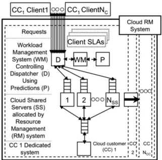
Based on[13,14,17]a cloud customer (CC) pays for shared servers (SS) which may be dynamically shared with other CC

and which may be virtualised – seeFig. 1. Here, a SS is being transferred from CC1 to CC2; SS transfers are controlled by the

cloud infrastructure resource management system (RM). When there is more than one virtual server running on a physical

server, each virtual server is allocated a minimum percentage of the physical server’s resources. There areNCCCC, each of

which can also hire dedicated servers (DS). The internal structure ofCC1shows the enterprise system model for the paper.

Based on established work[11,15]this is modelled as a tier of heterogeneous application SS accessing a database/legacy

sys-tem. Based on the queuing network in IBM Websphere: a single FIFO queue is used by each application server; the database server has one FIFO queue; and both types of server can process requests concurrently via time-sharing. The workload sists of clients (divided into service classes each with a SLA) which send requests to the system. The dispatcher (D), con-trolled by the cloud customer workload management system (WM), adjusts the routing of the incoming requests to the application servers. The algorithms in the management systems may use a prediction engine (P) to help make decisions, and may co-ordinate the use of these predictions e.g. between the resource and workload management systems. A cloud cus-tomer can run an urgent system which can make urgent requests for resources (e.g. for emergency response). For a detailed

survey and discussion of cloud environments and associated issues see[17].

2.2. Case study

The case study is based on the Eucalyptus[13]cloud model, with every CC either having this enterprise system model or

it is an urgent system. IBM Websphere is selected as the enterprise system middleware as it is a common choice for

distrib-uted enterprise applications; the IBM Performance Benchmark SampleTrade[16]is selected as it is the main enterprise

benchmark for the Websphere platform. The sample enterprise workload is as follows based on Trade and[11]. A service

class is created forbrowseusers withnbrowseclients, with the operation (buy/quote, etc.) called by a client being randomly

selected using the probabilities deﬁned by Trade. A service class withnbuyclients is created forbuyusers which involves

(4)

clients making an average of 10buyrequests. The percentage ofbuyclients is deﬁned asb. Think-times are exponentially

distributed based on[9] with a mean of 7 s for all service classes as recommended by IBM for Trade clients, although

heterogeneous think-times are supported by both techniques. Based on the Trade benchmark, atypical workloadis deﬁned

as allbrowseclients.

FireGridis a command and control application for urgent emergency response during a building fire. In experiments so far the majority of the processing has been to run embarrassingly parallel fire models so it is this which is run on the cloud. FireGridis selected as the urgent system as it is the result of significant and ongoing development by a large coalition includ-ing emergency response services and it has been tested in real-time durinclud-ing a live fire test featurinclud-ing a full-size mock-up of a three room flat.

2.3. Experimental setup and sample cloud

The experimental setup contains three application server architectures. Under Websphere v4.0.1. and the typical

work-load (deﬁned in the last sub-section) the max. throughputs of the new ‘slow’AppServS(P3 450 Mhz); the established ‘fast’

AppServF(P4 1.8 Ghz); and the established ‘very fast’AppServVF(P4 2.66 Ghz) are 86, 186 and 320 requests/s respectively. Each server is virtualised using a JVM. The database server architecture is DB2 7.2 on an Athlon 1.4 Ghz and 250 clients are simulated by each workload generator (P4 1.8 Ghz). The clients are simulated using an Apache JMeter script as described

in[6], with the workload being sampled to check it is being generated as required. All servers run Windows 2000, have at

least 512 MB RAM and are connected via a 100 Mbps switch.

In the sample cloudNCC= 4 withFireGridasCC4, andCC1,CC2andCC3are dynamic enterprise systems.CC1has one SS of each

of the three application server architectures and a workload of 3000 clients. Three service classes are created by dividing the browseservice class into two service classes with different SLA response time goals (RTG). The workload that is to be allocated

to the SS is deﬁned as 10%buyclients (RTG = 150 ms), 45% high prioritybrowseclients (RTG = 300 ms), and 45% low priority

browseclients (RTG = 600 ms). The percentages are selected based on the Trade application, which deﬁnes 10% of the standard workload to be purchase requests. The response time goals are selected based on the response time of the fastest application

server at max throughput (aprox 600 ms).CC2has 20% more clients, RTG all 20% lower and hence all servers upgraded to the

next fastest server architecture available (exceptingAppServVF– the fastest) to 2AppServVFand 1AppServF. ForCC3the

num-ber of clients and RTG ﬁgures are increased/decreased by an additional 20% respectively, and the SS are upgraded again

result-ing in 3AppServVF.CC4has all the other SS, in this case 5; the minimum number we have executed this part ofFireGridon.

3. Deﬁnition and experimental investigation of the layered queuing prediction model

This section describes the experimental investigation of the level of support provided for adynamic-urgent cloud

environ-mentusing a layered queuing prediction model, examining the associated overheads and hence providing guidelines on the

parameterisation of the model.

The layered queuing method involves deﬁning an application’s queuing network. An approximate solution to the model can then be generated automatically using the LQNS solver. The solution strategy involves dividing the queues into layers (e.g. as in the enterprise system model), generating an initial solution and then iterating backwards and forwards through the layers solving the queues in each layer by mean value analysis and propagating the result to the next layer until the solu-tions converge. Performance metrics generated include mean response time, throughputs and utilisation information for

each service class. A detailed description of the layered queuing method can be found in[9,23].

We have created a layered queuing model of an enterprise system withapp_svr,DB_svrandDB_svr_disklayers, each layer

containing a queue and a processor. The application server disk is not modelled as the Trade application’s utilisation of this

resource is found to be almost 0 during normal operation. Workload parameters for each service class

_v

are: the number of

clientsn_v; the mean processing times (on each processorp), t(p,v) ort(p,v)Nfor established and new server architectures

respectively; and the mean number of requests to the next layery(app_svr,v)andy(DB_svr,v). Processing times are exponentially

distributed as standard with the layered queuing method. Communication time is a constant delayd. Queue parameters per

layerlare the maximum number of requests each processor can process at the same time via time-sharingml.

Model parameterisation is as follows.dis parameterised by subtracting the predicted response time from the actual

re-sponse time at a small number of clients (250 in the experimental setup) on an established server. Then for eachpand for

each

v

take an established server off-line and send a workload consisting only of

v

for an interval. This overcomes the

dif-ﬁculties that have been found measuring mean processing times (without queuing delay) of multiple service classes, in real

system environments[15].t(p,v)is then calculated by dividing the associated mean interval server (or disk) CPU (or disk)

usage by the mean interval throughput (in requests/s). Calculatingt(p,v)Ninvolves multiplying a value oft(p,v)by the

estab-lished/new server request processing speed ratio. 3.1. Experimental results

In the remainder of this section we examine the predictive accuracy and resource usage overhead when parameterising the request processing times under different workloads. This includes an analysis on the effect of the number of clients used

(5)

to parameterise the mean processing time variables in the model. In the experimental setup (from Section2)mapp_svr= 50,

mDB_svr= 20,mDB_svr_disk= 1,yapp_svr,buy= 2 andyapp_svr,browse= 1.14.yDB_svr,vis modelled as 1 by setting the throughput of

DB_svr_diskto the throughput ofDB_svrduring parameterisation. The typical (browse) workload is parameterised on an

established application server with a max. throughput of 213 requests/s; for brevity we refer to the associated processor

asE. Each test run involves settingnbrowseand after a 1 min warm-up recording %CPU/disk usage samples and server mean

throughputs for 1 min. The sampling interval is set at 6 s so the increase in the %CPU/disk usage is no more than 5%. We

de-ﬁne predictive accuracy as the following. Note that in this paper the termaccuracyrefers to the accuracy of the predictions

(i.e. when compared to the measured data), as opposed to the accuracy of the measured data – unless this is explicitly stated. accuracy¼jpredicted

v

aluemeasured

v

aluej

measured

v

alue 100 ð1Þ

Asnbrowseis increasedt(E,browse)decreases (from 5.6 ms atnbrowse= 63) to a minimum of 4.3 ms atnbrowse= 750. It then

in-creases (to 4.7 ms atnbrowse= 2250). This pattern is explained as follows. The higher mean processing times at smaller

num-ber of clients are due to the larger system and JVM overhead (i.e. for garbage collection) per request. The higher mean processing times at larger numbers of clients are due to the overhead of running a larger number of threads (as Websphere terminates threads that are not needed, at lighter loads). At intermediate numbers of clients these overheads are less signi-ﬁcant resulting in lower mean processing times. As a result the predictive accuracy is highest when parameterising the

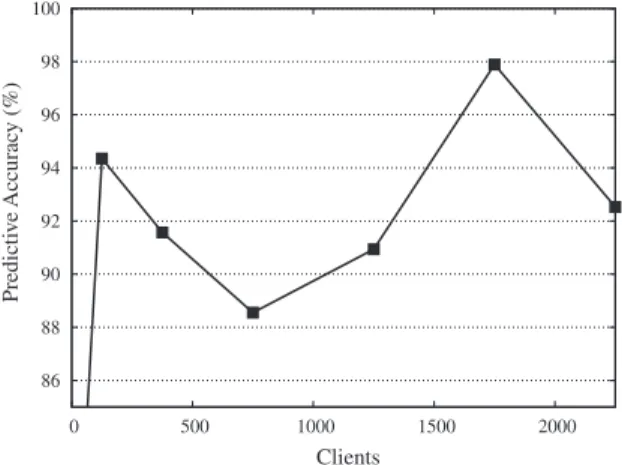
mod-el at a value ofn_vbetween the maximum and minimum mean processing times – seeTable 1. However, the highernbrowsethe

more server capacity that must be taken off-line to run the workload generators, application and database servers. The

max-imum predictive accuracy when the model is parameterised at a low overhead is atnbrowse= 125; below this the predictive

accuracy drops signiﬁcantly. This is due to a discontinuity in the rate at which the mean response time increases with num-ber of clients around the point at which max. throughput is reached. The predictive accuracy around this point (one of the predictive accuracy measurements taken at different numbers of clients so as to calculate, via a mean the predictive accu-racy) is less accurate than for other numbers of clients. Hence the predictive accuracy at the ﬁrst maximum is slightly lower

than that of the second maximum. Whennbrowse= 125 thent(E,browse)= 4.675 ms,t(F,browse)= 1.821 ms andt(G,browse)= 0.638 ms

whereFis the database server processor andGis the database server disk processor. This results in a predictive accuracy of

80% on the new server architecture – seeTable 2andFig. 2. We note that in previous work[4,6]we have shown how

per-centile response time metrics can be predicted based on the measured exponential distributions. To parameterise the model a server capacity of 89 requests/s must be taken off-line for 2 min per service class. This is the equivalent of a Pentium III 450 Mhz which is likely to be a low parameterisation overhead for a modern resource management system. It is also impor-tant to consider the delay when solving the model. Using the standard LQNS solver on a dedicated Athlon 1.4 Ghz at a con-vergence criterion of 20 ms this is observed as follows. When the server is lightly loaded and when the server is saturated the model can be solved in around 1 s. However, as you move away from these two extremes the time to solve increases up to a maximum of 5 s. This point is reached just before 100% of the number of clients at max. throughput. However, most of the

predictions are made in 1–3 s. The consequences of these evaluation times are discussed in Sections5 and 6.

3.2. Guidelines for parameterising the model at a low overhead

We have found that frequent, rapid model parameterisations can be useful for maintaining predictive accuracy in dy-namic enterprise systems – assuming this is used with care. For example correcting for predictive inaccuracy by paramete-rising again can mask the need for reﬁnements in the conﬁguration of the enterprise system/cloud/model etc. It is also important to check the predictive accuracy of the model immediately after parameterisation as it may occasionally be nec-essary to repeat the parameterisation, for example after a brief spike of background activity.

Table 1

The predictive accuracy when parameterising the layered queuing model at different numbers of clients as shown inFig. 2.

No. of clients 63 125 375 750 1250 1750 2250

Predictive accuracy (%) 84.60 94.35 91.57 88.55 90.94 97.89 92.53

Table 2

Response time predictions for the new server architecture.

No. of clients 250 500 750

Measured mean (ms): 122.9 210.4 2060.2

Layered queuing predicted mean (ms): 105.9 137.4 1811.3

Layered queuing predictive accuracy (%): 86.2 65.3 87.9

Historical predicted mean (ms): 139.1 268.7 2581.8

(6)

Our guidelines for parameterising the layered queuing method are as follows based on the experimental analysis in

Sec-tion3. The key variable isnv, the number of clients at which the layered queuing model is parameterised for each service

class

v

. This is because the layered queuing method assumes that the per service class request processing times (t(p,v)) are

constant at different server loads. However this was not found to always be the case due to system (i.e. garbage collection)

and thread overheads at small and large numbers of clients, respectively. Asn_vand hence the server load is increased, so does

the parameterisation overhead. We have found that there tends to be a minimum number of clients that gives a high

accu-racy and low overhead (e.g.nbrowse= 125 clients in our setup – seeTable 1). The procedure in Section3should be used to

identify this point. Alternatively if spare machines are available to parameterise the model the procedure can be used to

locate the high overhead parameterisation point that gives the maximum accuracy (seeTable 1).

The implications of the layered queuing model experimental results presented in this section are discussed further in

Sec-tion6.

4. Deﬁnition and experimental investigation of the HYDRA historical prediction model

This section describes the experimental investigation of the level of support provided for adynamic-urgent cloud

environ-mentusing a (‘HYDRA’) historical prediction model, examining the associated overheads and hence providing guidelines on

the parameterisation of the model.

The historical modelling technique[4–6]involves sampling performance metrics and associating these measurements

with variables representing the workload being processed and the machine’s architecture. Historical models then deﬁne the relationships (e.g. linear/exponential equations) between the variables and metrics. In the case study, the server

work-load variables are the number of clientsnand the percentage ofbuyclientsb. The main server architecture variable is request

processing speed (measured as max_thr, the max. throughput under the typical workload, in these experiments). Let

no_of_clientsmtbe the number of clients atmax_thr.Relationship 1models the effect ofno_of_clients, the number of typical workload clients, on the mean response time. It has been found that this relationship is best approximated using separate

lower and upper equations – see Eqs.(2) and (3)respectively. A middle equation (not shown for brevity) the same as

Eq.(2)withLreplaced byM.

mrtL¼cLeðkLno of clientsÞ ð2Þ

mrtU¼kUno of clientsþcU ð3Þ

where mrtL/mrtU is the mean response time for when no_of_clients< (0.75no_of_clientsmt) and no_of_

cli-ents> (1.1no_of_clientsmt) respectively, andcL,cM,cU,kL,kMandkUare parameters that must be parameterised from

histor-ical data.no_of_clientsmtis calculated using a relationship betweenno_of_clientsand the server throughput (see[4]). We have

also found, although it is not covered in this paper, that using a transition relationship to phase between the lower and

mid-dle, or middle and upper equations can increase predictive accuracy[5].

Relationship 2models the effect ofmax_thronrelationship 1as follows:

cL¼

K

ðcLÞ max thrþCðcLÞ ð4Þ

kL¼Cð

K

LÞ max thrKðkLÞ ð5Þ

whereK(cL),C(cL),C(kL) andK(kL) are parameters that must be parameterised from historical data. For brevity equations for

the middle equation (Eqs.(4) and (5)withLreplaced byM) are not shown. The equations for parameters for the upper

(lin-ear) equations are calculated as follows. Given an increase/decrease inmax_throfz%,kUis found to increase/decrease by

roughly 1/z%, andcUis found to be roughly constant.

86 88 90 92 94 96 98 100 0 500 1000 1500 2000 Predicti v e Accurac y (%) Clients

(7)

Relationship3 models the effect ofbonmax_thr; this is found to be a linear relationship. This is used to extrapolate

max_thrE(b), the max. throughput of an established server under b. The max. throughput on a new server under b,

max_thrN(b), is then calculated using Eq.(6), whereb= 0 represents the typical workload.

max thrNðbÞ ¼

max thrEðbÞ

max thrEð0Þ

max thrNð0Þ ð6Þ

4.1. Experimental results

The remainder of this section experimentally investigates the parameterisation of historical models on a live system,

using the experimental setup from Section2. This allows an historical model to be parameterised at a signiﬁcantly smaller

resource usage overhead than the layered queuing method as the only additional requirement on the system is to process the

one (or more) response time sampling clients. The parameters inrelationship1 andrelationship2 are parameterised by ﬁtting

least squares trend-lines to historical data from the establishedAppServFandAppServVFservers. The historical data consists of

themax_throf each server anddpdata points for each equationq(either ‘upper’, ‘middle’ or ‘lower’) ofrelationship 1

respec-tively. Each data point recordsno_of_clientsand themrtq(averaged acrossssamples) for the typical workload.

The overall predictive accuracy is deﬁned as the mean of the lower, middle and upper equation predictive accuracy. It is

found that accurate predictions can be made even whendpis reduced to 2 andsis reduced to 50. The resulting parameters

are shown inTables 3 and 4. A good level of predictive accuracy of 94% and 78% for the established/new server architectures

respectively is achieved (seeTable 2).Relationship3 can be rapidly parameterised as this only requires one additional item of

data;max_thrE(b) for ab> 0. This is tested using LQNS predictions for historical data, speciﬁcallymax_thrE(25) = 158

(re-quests/s) forAppServF. The resulting predictive accuracy is 74% on the new server architecture. Once Eqs.(2)–(6)have been

parameterised predictions can be made almost instantaneously.

Having calculated the predictive accuracy, it is necessary to calculate the overheads that were incurred. The total

sam-pling timetrequired to parameterise the model (that is, the time to parameterise the model using one instrumented client)

is estimated in Eq.(7)wheresi,riandhiare the number of samples, mean response time and mean think-time when

record-ing data pointi, andDPis the total number of data points. Sinceriwill not be known (and cannot be predicted) until after the

model has been parameterised it is not normally possible to predict in advance exactly how long the parameterisation will

take. However,rican be estimated, for example by using the measurements/predictions from the previous parameterisation

or, in the case of a new application, from when the application was being tested prior to deployment. Since distributed

enter-prise think-times can be quite long (for example 7 s as recommended by IBM for Trade clients)tcan be quite large. For

exam-ple in this case the parameters areDP= 6 for each of the two server architectures, andsi= 50 andhi= 7000 ms for each data

point. The historical model parameter values are used as therparameters. This results int= 76 min.

However, by using multiple simulated clients to sample the response times this can be dramatically reduced. When using

csimulated clients to record each data point the resource usage overheadoon the system can be calculated by Eq.(8)where

liis the total number of clients for data pointi. For these predictionscis set to 12 so that the maximum resource usage

over-head for a data point is 5% (for data points recorded at 250 clients). The resulting overall resource usageois calculated at 1.8%

forAppServFand 0.91% forAppServVF; a low overhead. The overhead is less forAppServVFas it is a more powerful server

archi-tecture. Alternatively the value ofccould be increased so as to parameterise the model more rapidly, albeit at a higher

re-source usage overhead. The time to parameterise the model whenc> 1 is calculated as Eq.(9).

In this case this results in a time to parameterise of 3 min 12 s forAppServFand 3 min 9 s forAppServVF. In these

exper-iments the system was warmed up for 30 s prior to recording each data point, creating an additional overhead of 3 min for each server. However, due to the high throughputs of the systems under parameterisation (35–320 requests/s) it is likely that the system reaches a steady state more rapidly than this and so this warm-up interval could be reduced. Indeed it is likely to be particularly effective to base the duration of this warm-up interval on the server throughput, with shorter warm-up times for higher throughput data points. Overall these calculations show that the historical model can be rapidly parameterised at a low resource usage overhead.

Table 3

Calculated parameters for the new server architecture.

cL kL cM kM cU kU

138.9 4E06

51.6 0.0033 7573 13.54

Table 4

Calculated parameters used to calculate the predictions inTable 2.

K(cL) C(cL) C(kL) K(kL) K(cM) C(cM) C(kM) K(kM)

(8)

t¼X DP i¼1 siðriþhiÞ ½ ð7Þ o¼ PDP i¼1 si lci h i PDP i¼1si 100 ð8Þ t¼X DP i¼1 si c l m ðriþhiÞ h i ð9Þ

4.2. Guidelines for parameterising the model at a low overhead

Our guidelines for achieving accurate predictions at a low overhead using the historical technique are as follows based on the experimental analysis in this section. It is necessary to sample the response times of established servers at a range of

loads for the lower, middle and upper equations ofrelationship 1. This is due to the changing shape of the response time

graph as server load increases (see[4]). It is also necessary to use two (or more) established application server architectures

for parameterisation so as to be able to extrapolate a trend-line (unlike the layered queuing method which only requires one). Further, when sampling the response times of an established server for the lower, middle or upper equations it is nec-essary to include samples at both low and high numbers of clients so as to get a sufﬁcient spread of data points from which to draw a trend-line. Initial experiments have shown that exponential predictive accuracy increases signiﬁcantly if three or more (number of clients, mean response time) data points are used for parameterisation as opposed to the current two. We therefore recommend that a minimum of two/three data points (with at least 50 samples per data point) be used when parameterising linear/exponential trend-lines, although in practice the more data points used the better.

The implications of the historical model experimental results presented in this section are discussed further in Section6.

5. Experimental investigation of using prediction models in a cloud workload and resource management system

Sections3 and 4have experimentally investigated the level of support for dynamic-urgent cloud environments provided

by the layered queuing model and HYDRA historical model respectively. This has included showing that rapid predictions can be made for an enterprise application on a new server architecture in a dynamic-urgent cloud environment with a good level of predictive accuracy. These sections have also shown that this can be achieved despite rapidly parameterising the model at a low overhead. We now move onto experimentally investigate the use of these prediction models by the manage-ment systems of both the cloud (i.e. the resource managemanage-ment system) and cloud customer (i.e. the workload managemanage-ment system). Using the historical and layered queuing models in this section we deﬁne a cloud resource and workload manage-ment algorithm that uses simulations as part of the decision-making process. We then experimanage-mentally investigate via sim-ulation the effectiveness of this algorithm in different operating scenarios. This includes how a prediction-enhanced workload and resource management algorithm can be tuned, and the deﬁnition, implementation and experimental investi-gation of an algorithm that does not use predictions.

SLA-based cloud customers running enterprise systems (as deﬁned in Section2) incur two main types of cost. The ﬁrst

in-volves paying penalties for SLA failures e.g. missing SLA response time goals; and the second is the cost of using the servers in

the system. %_SLA_failuresis deﬁned as the percentage of clients rejected from the server/s of a cloud customer (CC) and %_

ser-ver_usageis deﬁned as the percentage of the total cloud shared server (SS) processing power (SSPP) allocated to a CC, with

pro-cessing power deﬁned asmax_thr. A generic strategy to compensate for predictive inaccuracy and balance the cloud customers’

costs involves running the resource and workload management algorithm, as if the cloud customers’ workloads are larger than

they actually are. In these experiments this involves multiplying the number of clients in each service class in each CC byslack.

Some service classes may have insufﬁcient servers for %_SLA_failures= 0 to be achieved, e.g. due to predictive inaccuracy.

To deal with this the enterprise system model in Section2is extended so application servers reject clients at runtime if

re-sponse times are within a threshold of missing SLA goals. It is assumed these clients miss their SLA goals. This prevents all the existing clients on a server from also missing their SLA goals. In practice, it is likely that the rejected workload would be handled by a second set of servers in the cloud for each CC, that accept all workload for that customer.

The historical and layered queuing models are used in these experiments as follows. The layered queuing method can require signiﬁcant CPU time to make each mean response time prediction (i.e. up to 5 s on an Athlon 1.4 Ghz under a con-vergence criterion of 20 ms). Further, multiple predictions must be made to make the reverse prediction i.e. searching for the maximum number of clients an SLA compliant server can support. This is information that may be requested frequently by workload and resource management algorithms and can be provided almost instantaneously by the historical model. A workaround to this problem is to ﬁt trend-lines to the layered queuing mean response time predictions (using historical

modelrelationship 1only) and use these to make all predictions almost instantaneously, albeit at the cost of a 1.7% reduction

in predictive accuracy. This reduction is very small in part because of the absence of experimental noise. In the experiments in this section these ‘hybrid’ predictions are used as the predictions and the more accurate historical model is used as the real system response times so as to be able to provide the workload and resource management algorithm with all the required data.

(9)

5.1. Deﬁning the workload and resource management algorithm

Algorithm 1is our cloud resource and workload management algorithm for use when there is no suitable unallocated server processing power available to process an urgent application. The algorithm reassigns servers from one CC to another

and assigns workload to servers. In the experiments in this paper the functionselectCandidateCC(CCx,p,. . .) returns all the

cloud customers exceptCCxand functionselectCandidateServers(c,. . .) returns all SS incunless a SS has already been

allo-cated from this CC in which case no SS are returned. Step 9 is implemented by the resource management algorithm (RM)

repeatedly searching the set of tuples generated by step 7 for the tuple with the lowest value ofm, and removing that tuple

and the corresponding shared server; this repeats until ((SSPP_removed)Pp) or there are no more tuples, whereSSPP_

re-movedis the shared server processing power removed.

Algorithm 1. Distributed resource and workload management algorithm.

1: Cloud customer (CC)CCxrequestspshared server processing power (SSPP) from the cloud resource management

system (RM).

2: RM executescc=selectCandidateCC(CCx,p,. . .) to select a set of CC it might take SS from, using the policy set by the

cloud administrators.

3: RMgathers information by asking the workload management system (WM) in each (CCcincc) to predict the effect

on their %_SLA_failuresof losing: 1 SS; 2 SS; up tomin(p,spp(c)) SSPP.spp() is a function returning the total SSPP of a

CC or server. The WM for each CCcinccsends the information by:

4: parameterise predictions model, copy conﬁguration ofcinto new workload transfer algorithm (WTA) simulation

simc.

5: for all SSsinselectCandidateServers(c,. . .) do

6: copysimcintosimc,sand use this to simulate transferring the workload fromsonto the other SS inc, removingsfrom

c, and then (assuming at this stage accurate predictions) predict the resulting %_SLA_failure fc,s.

7: end for

8: The serverswith the lowest value ofm=fc,s/spp(s) is selected. Deletesimcand renamesimc,stosimc. Send (c,s,fc,s,m)

to RM.

9: RM selects set of CC and decides on SSPP to take from each.

10: For each selected CCc, the WM tells its dispatcher, for each SS it is to lose, to transfer workload off it as persimc. As

SS become idle they are transferred toCCxby RM.

The workload transfer algorithmWTAprovides, for a cloud customerc, an allocation of workload to a set of servers using

information provided by a performance model, calculating the resulting %_SLA_failuresand %_server_usage. Since there is

no priority queuing or processing in the system model, ourWTAaims to avoid workload with different SLA response time

goals on the same server. To improve execution time ourWTAexecutes as follows: (i) work through the service classes in

order of priority; (ii) for each service class compile a setbpof the best possible servers for the workloadwin the current

service class; and then allocatewto the servers inbpbeing considerate to other service classes. The algorithm is shown

inAlgorithm 2. OurWTAsimulation can, given data representing the real performance of the servers, calculate the resulting %_SLA_failuresand %_server_usage. Each service class consists of a number of clients, each of which is initially unallocated. Application servers are considered to have available capacity unless the performance model predicts that adding an extra client from the current service class would result in some clients missing SLA response time goals.

Algorithm 2. Workload transfer algorithm WTA.

1: Sort the service classes in order of increasing response time goal.

2: Let current_service_class = ﬁrst service class in list

3: repeat

4: if all clients in current_service_class allocated to an application server

then

5: current_service_class = next service class in list

6: end if

7: app_server = application_server_selection_algorithm ()

8: repeat

9: allocate clients from current_service_class to app_server

10: until maximum capacity is reached on app_server OR all clients in current_service_class are allocated to an application server

(10)

5.2. Example use of predictions in a cloud workload and resource management system

This sub-section describes an example use ofAlgorithm 1using the sample cloud from Section2. We useWTAto allocate

each CC workload onto the SS belonging to that CC. We observe that for all CC there are no %_SLA_failures.FireGrid(CC4) then

requests the equivalent of 3AppServSworth of shared server processing power (SSPP) (i.e.p= 258 requests/s). This is to

takeFireGrid’s number of SS up to 8 – our standard number for a small ﬁre (e.g. in one room). We runAlgorithm 1with slack= 1 (i.e. no predictive accuracy compensation). For each ofCC1andCC2there is one SS for whichm= 0 – seeTable 5.

This means the predictions indicateFireGridcan be given the required servers without causing any %_SLA_failures, once

WTAis used for each CC to re-allocate the displaced workload. (This is not the case forCC3;m= 0.022 soCC3is not considered

further.) However there is a (non-uniform) predictive inaccuracy so some %_SLA_failuresoccur.Table 5shows how setting

slack= 1.1 (which results in the samemvalues of 0) signiﬁcantly improves this. However increasing the slack too far can put too little workload on some of the SS and hence be less effective at reducing SLA failures. An example of this on the

se-lected two servers is shown in the last line ofTable 5for whenslack= 1.2. The value ofslack= 1.1 is found by manual

exper-imentation. This approach is selected as we have found experimentally that if predictive accuracy is uniform it can be

straightforward to calculate a good value ofslackbut in more realistic scenarios manual experimentation is often a good

ap-proach[4].

5.3. Experimental investigation of the effectiveness of prediction-enhanced workload-resource assignment in different operating scenarios

The remainder of this section experimentally investigates the effectiveness of prediction-enhanced workload-resource assignment in different operating scenarios. We have found in previous experiments that there are three important operat-ing scenario variables to cover when investigatoperat-ing the effectiveness of a prediction-based management system: (1) the ex-tent to which the system is loaded; (2) the scenario heterogeneity; and (3) whether the performance predictions are tuned to

compensate for predictive inaccuracy[4,20]. We therefore investigate these variables. This study builds on our analysis of

tuning SLA failure versus resource usage in a prediction-based management system[4]. The experimental setup is extended

to include a total of 16 application servers. Eight of the servers have a new architecture (AppServS) and eight have the same

architectures as existing servers (fourAppServFand fourAppServVF) 100% resource usage is deﬁned as using all 16 servers.

Algorithm 3. No prediction workload-resource assignment algorithm.

1: Let total_processing_power = sum of processing powers for all servers.

2: Calculate the proportion of total_processing_power allowed to go to each service class by weighting each service

class in inverse proportion to its SLA goal. Assign this to service class variable allowed_processing_power.

3: Let unallocated_processing_power = server_processing_power

4: Let servers = all servers ordered by processing power

5: for all server in servers do

6: Select the highest priority service class with allowed_processing_power–0.

7: Allocate as much processing power to this service class as it is allowed (or until the server runs out of

unallocated processing power) and hence proportionally allocate clients from that service class to the server. 8: end for

Algorithm 3shows our workload-resource assignment algorithm that does not use predictions, based in part on one of the algorithms that comes as standard in the IBM Websphere platform. In these experiments we compare this algorithm to the prediction-enhanced algorithm. We note that the weighted allocation of workload to servers could be further reﬁned by also weighting by service class mean request processing time. However this is not done here due to the difﬁculties that have been found measuring mean processing times (without queuing delay) of multiple service classes, in real system environments

[15]. The processing power of each server is measured as the maximum throughput of the server under the typical workload.

We begin the experiments using the workload from Section2, which we refer to as the standard workload. The average

predictive accuracy of the (non-uniform) predictions (weighted by the number of servers in the server pool) is 92.5% (cor-Table 5

Workload and resource management results.

Cloud customer (CC) 1 2

Server architecture taken AppServS AppServF

Server speed (requests/s) 86 186

%_SLA_failures(slack= 1.0) 0.0 2.64

%_SLA_failures(slack= 1.1) 0.0 0.25

(11)

responding to a slack of 1.075). However the minimum slack that results in 0% SLA failures before 100% resource usage is 1.1. The difference is due to some predictions being used more by the prediction-enhanced algorithm than others. For example

the predictive accuracy ofAppServFis the highest of the three servers at 97.04%, but due to the design of the

prediction-enhanced algorithm the middle servers tend to be used less frequently. We set the slack at 1.075 as we have found that allowing for a small number of SLA failures at about this level can result in a disproportionately large improvement in

the % resource usage[4].

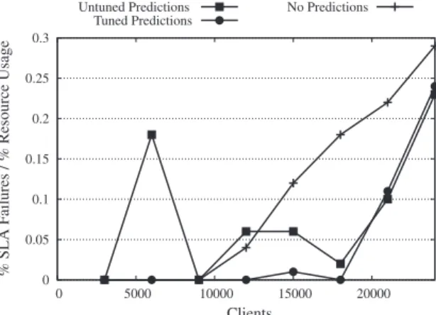
Table 6andFig. 3show the results. It can be seen that the tuned prediction-enhanced algorithm signiﬁcantly outperforms the no prediction algorithm. However if the prediction-enhanced algorithm is not properly tuned its performance is much more variable and at some numbers of clients performs worse than the no prediction algorithm. It is noted that the irregular shape of e.g. the ‘not tuned’ line is because runtime optimisations allow the system to use any available capacity the algo-rithm leaves on a server. So, once the total workload crosses a threshold and a small number of clients are allocated to an additional server, the performance will temporarily improve (as can be seen at 9000 clients).

For the next set of results we create a workload in which the mean buy service class SLA response time goal (RTG) is di-vided by two (so RTG = 75 ms). In addition, the low priority browse service class RTG is doubled (so RTG = 1200 ms). We refer to this as the more heterogeneous workload. The tuning is not modiﬁed since being set based on the standard workload. The

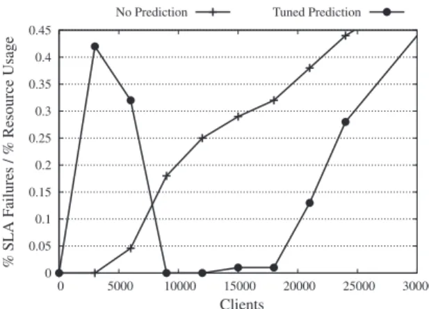
results for the more heterogeneous workload are shown inTable 7and graphed inFig. 4. It can be seen that at small numbers

of clients the tuned prediction-enhanced algorithm does signiﬁcantly worse than the no prediction algorithm. This illustrates

Table 6

% SLA failure per % resource usage at different numbers of clients for the standard workload as shown inFig. 3.

No. of clients Using predictions (not tuned) Using predictions (tuned) No predictions

3000 0.00 0.00 0.00 6000 0.18 0.00 0.00 9000 0.00 0.00 0.00 12,000 0.06 0.00 0.04 15,000 0.06 0.01 0.12 18,000 0.02 0.00 0.18 21,000 0.10 0.11 0.22 24,000 0.23 0.24 0.29 0 0.05 0.1 0.15 0.2 0.25 0.3 0 5000 10000 15000 20000 % SLA F

ailures / % Resource Usage

Clients Untuned Predictions

Tuned Predictions

No Predictions

Fig. 3.% SLA failure per unit resource usage at different numbers of clients for the standard workload.

Table 7

% SLA failure/ % resource usage at different numbers of clients, for the more heterogeneous workload as shown inFig. 4.

No. of clients No prediction Prediction (tuned)

3000 0 0.42 6000 0.046 0.32 9000 0.18 0 12,000 0.25 0 15,000 0.29 0.01 18,000 0.32 0.01 21,000 0.38 0.13 24,000 0.44 0.28

(12)

the importance of considering a range of likely operating scenarios when manually tuning the prediction-enhanced

algo-rithm. In this instance the value ofslackset using the standard workload is too low and should be increased – albeit at

the cost of a small increase in % resource usage.Table 7also shows how the no prediction algorithm does signiﬁcantly worse

under the more heterogeneous workload. This is discussed further in Section6.

An important difference between a properly tuned) prediction-enhanced algorithm and a no prediction algorithm is as follows. With the prediction-enhanced algorithm as the number of clients increases, ﬁrst all the lowest priority service clas-ses fail their SLAs, then the next lowest priority service class etc. In contrast there is only limited control of the order (and extent) to which the service classes are effected as the number of clients increases, in the no prediction algorithm. That is, higher priority service classes can be put on faster servers with established server architectures, but this does not give any

guarantee. The SLA failure per service class results for the standard workload are shown inTables 8 and 9. Service classes

with no SLA failures for the data range shown on each graph are removed for clarity. For the no prediction algorithm the SLA failures for smaller numbers of clients are from the low priority browse service class. However once the % SLA failures for this service class reaches just under 50% the high priority browse service class starts to suffer SLA failures. In contrast it is not until the prediction-enhanced algorithm reaches 100% SLA failures for the low priority browse service class, that the high priority browse service class starts to suffer SLA failures.

In summary this section has experimentally investigated the effectiveness of using performance predictions in different operating scenarios. These operating scenarios have been selected as those our previous work has identiﬁed as important

when investigating the effectiveness of performance predictions[4,20]. The implications of the experimental results

pre-sented in this section are discussed further in Section6.

6. Evaluations, guidelines and discussion

In this section, based on the experimental investigation in Sections 3–5, we: (i) provide a critique of the layered

queuing and historical methods and the application of these methods in this paper; (ii) evaluate the effectiveness of 0 0.05 0.1 0.15 0.2 0.25 0.3 0.35 0.4 0.45 0 5000 10000 15000 20000 25000 30000 % SLA F

ailures / % Resource Usage

Clients

No Prediction Tuned Prediction

Fig. 4.% SLA failure per unit resource usage at different numbers of clients, for the more heterogeneous workload.

0 20 40 60 80 100 0 5000 10000 15000 20000 25000 30000 35000 40000 % SLA F

ailures per Service Class

Clients

Predictions, Low Priority Browse SC, Tuned Predictions, High Priority Browse SC, Tuned

(13)

the prediction-enhanced workload and resource management algorithm from Section5in differentdynamic-urgent cloud environmentoperating scenarios; and (iii) provide guidance on using a prediction-based workload and resource

manage-ment algorithm in adynamic-urgent cloud environment.

6.1. Critique of the layered queuing and historical methods and the application of these methods in this paper 6.1.1. Critique of the layered queuing and historical methods

We have provided a detailed critique of the historical and layered queuing methods and their application under ﬁve

eval-uation criteria in[6]. This includes both model description and analysis. Overall, there is no clear modelling paradigm of

choice as the historical method and layered queuing method are strong under different evaluation criteria. Four of these evaluation criteria (systems that can be modelled, metrics that can be predicted, ease of use given a minimal level of per-formance modelling expertise and prediction responsiveness) are evaluated qualitatively based on the underlying character-istics of the two methods.

Table 8

% SLA failure per service class (SC) at different numbers of clients, for the standard workload with the prediction-enhanced algorithm as shown inFig. 5. No. of clients Predictions (tuned) (low priority browse SC) Predictions (tuned) (high priority browse SC)

3000 0.00 0.00 6000 0.00 0.00 9000 0.00 0.00 12,000 0.00 0.00 15,000 1.16 0.00 18,000 0.23 0.00 21,000 25.37 0.00 24,000 53.00 0.00 27,000 74.69 0.00 30,000 91.21 0.00 33,000 100.00 2.03 36,000 100.00 12.04 39,000 100.00 20.52 42,000 100.00 28.47 Table 9

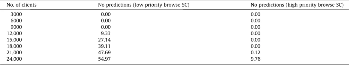
% SLA failure per service class at different numbers of clients, for the standard workload with the no prediction enhanced algorithm as shown inFig. 6. No. of clients No predictions (low priority browse SC) No predictions (high priority browse SC)

3000 0.00 0.00 6000 0.00 0.00 9000 0.00 0.00 12,000 9.33 0.00 15,000 27.14 0.00 18,000 39.11 0.00 21,000 47.69 0.12 24,000 54.97 9.76 0 10 20 30 40 50 60 0 5000 10000 15000 20000 % SLA F

ailures per Service Class

Clients

No Predictions, Low Priority Browse SC No Predictions, High Priority Browse SC

(14)

Some highlights are as follows. There are a number of functional limitations with the layered queuing method that should be taken into account when selecting a technique. It is more difﬁcult to model applications that cache signiﬁcant amount of

database data at the application server (as opposed to applications such as theTradebenchmark which access the majority

of database data directly so as to avoid data inconsistencies if the application server crashes). This is because the number of calls to the database must be a constant in the layered queuing model, whereas if a cache is used this value will depend on the cache miss rate. Using the historical technique the size of the application server’s cache can be recorded as an extra variable. Relationships can then be added to approximate the historical relationship between the performance metrics, this

new variable and the existing variables, using the techniques presented in Section4. Another limitation of the layered

queuing method is that the important class of percentile response time metrics cannot be predicted directly. In contrast the historical technique can extrapolate from and hence make predictions for a wide range of metrics.

However layered queuing models are also significantly easier to create with a minimum level of performance modelling expertise than a historical model. This is because creating a historical model involves specifying and validating how predic-tions will be made, whereas once a system’s queuing network configuration is specified layered queuing models can be solved automatically. The layered queuing method may therefore be preferable when there is a shortage of either time or performance modelling expertise when creating the model. The main conclusion under the ‘prediction evaluation delay’ cri-teria is that the historical method can be significantly more responsive than the layered queuing method. This is based pri-marily on the fact that the historical method supports runtime predictions made by a single equation such as (once

parameterised) Eqs.(2) or (3). However the procedure for solving a layered queuing model, as outlined in Section3, can

re-quire signiﬁcantly more resources to solve via, e.g. iteration or simulation. Indeed, this is what we have found in our

exper-imental experience (see results in Section3.1).

We also note that the historical technique has tool support primarily to help collect the historical data – however this is

aimed at expert users (see the HYDRA Toolkit[6]). The layered queuing method has tool support for both beginners and more

experienced users, including a model validator, solver and GUI editor. Further, although both techniques are well

docu-mented (e.g.[4–6,9–11]), it is once again only the layered queuing method that provides material for both beginner and

more expert users.

Our critique of the methods under the ‘high accuracy new server architecture predictions given low overhead parameteri-sation’ evaluation criteria is based in part on the underlying characteristics of the methods and in part on the quantitative

experimental results from this study. This is discussed further in Section6.1.2.

6.1.2. Critique of the application of the layered queuing and historical methods in this paper

This sub-section provides a critical discussion on the application of the layered queuing and historical methods in this paper (i.e. for model description and analysis). We have shown in this paper it is possible to make accurate new server archi-tecture predictions after only rapid low overhead parameterisation using both the layered queuing and historical methods. The following qualiﬁes this statement. A historical model may perform poorly if there are problems with the historical data e.g. due to the samples per data point being too small; the historical data not covering the full range of likely system states; there being insufﬁcient data points per model relationship; or due to experimental error. Both the analysis (for parameteri-sation) and model description rely on this historical data. We refer the reader to our analysis of the effect on the historical

model of insufﬁcient historical data[4,6]. We have found that some layered queuing models may be best solved via a

sig-niﬁcantly slower solver tool as opposed to the faster but potentially less accurate analytical approximation tool (LQNS) used in this paper (see also the note below about this tool). During layered queuing model analysis sources of parameterisation uncertainty include experimental error and the number of clients at which the model is parameterised – see the analysis in

Section3.1. See also[6]for further qualiﬁcations for both methods.

For a justiﬁcation and discussion of the main assumptions we make see[6]and elsewhere in this paper. We note in

par-ticular the following. We have validated our exponential service times assumption experimentally for the experimental

set-up – and this is sset-upported by, e.g.[10,11]. Our future publications will study metrics based on quantiles or higher moments.

This will be based in part on our initial results predicting percentile response times with a good level of accuracy, based on

predicted exponential response time distributions[6]. We have validated our experimental performance data and

experi-mental setup using manual checking, our layered queuing model and comparison to related studies[1,11,15].

See[6]for our detailed discussion of alternative performance predictions methods and alternative ways of applying the

layered queuing and historical models. For example, in our model description an alternative would be experimentally

inves-tigating variations (e.g. approximations) on the models in this study based on our initial results and guidance on this in[6].

This is particularly important with the layered queuing method as modelling variations can occasionally prevent the LQNS solver producing a prediction. Examples of potential alternative analysis include introducing additional noise artiﬁcially to parameterisation data; or doing extra analysis on the historical model by creating a hybrid of the historical and layered

queuing model (see[6]). This hybrid involves generating ‘pseudo’ historical (workload, performance) data points for a server

architecture using a layered queuing model, and using these data points to parameterise the relationships in a historical model. This is then used to make predictions which can be tested against the layered queuing prediction even if real histor-ical data is not available. Disadvantages include a reduction in predictive accuracy and having to create and parameterise two models.

We conclude by noting that we have chosen the historical and layered queuing methods – and the application of the methods described in this paper – because they are effective and we are familiar with them. Future work includes doing

(15)

sensitivity and transient analyses. This will be based on our previous analyses of the effect of key variables which can change

predictive accuracy. These include[4,6], Section3.1and our work on the effect of predictive inaccuracy in workload and

re-source management[21].

6.2. Evaluation of the effectiveness of the prediction-enhanced workload and resource management algorithm in different operating scenarios

This section considers the effectiveness of the prediction-enhanced workload and resource management algorithm in

dif-ferentdynamic-urgent cloud environmentoperating scenarios. This considers the prediction-enhanced workload and resource

management algorithm with both the layered queuing and historical models plugged in.

The more heterogeneous an operating scenario is (e.g. in terms of the workload and resources), the more unique options there are likely to be for how workload is allocated to resources. This is likely to give the prediction-enhanced algorithm an increasing edge over the no prediction algorithm as the system becomes more heterogeneous. For an illustration of this

effect see Fig. 4. This shows how the improvement the prediction-enhanced algorithm provides over the no prediction

algorithm is greater in the more heterogeneous operating scenario. It must also be considered that as the number of work-load-resource allocation decisions to consider (and hence the number of predictions required) increases, the management algorithm will require more resources to calculate predictions. This will be particularly noticeable when using layered queu-ing predictions, and may be almost unnoticeable when usqueu-ing historical predictions on small clouds. For example, in the experiments in this paper, assigning a workload with three service classes to a set of 16 servers using the historical model took only a maximum of a couple of seconds to complete. An additional consideration is that in operating scenarios that are consistently very homogeneous there may be a shortage of historical data for the historical model to extrapolate from. For example, if predictions are required urgently to evaluate unusual system changes being considered by the workload and resource management system.

In increasingly lightly loaded operating scenarios, the costs of using predictions for workload and resource management are increasingly likely to out-weigh the beneﬁts. In an operating scenario that is so heavily loaded the system is almost sat-urated, predictions may not be able to stop the system having undesirable levels of performance. However, they are likely to be useful in other regards – for example, in more precisely controlling which parts of the workload suffer. An example of

these behaviours is presented in the per service class results in Section5.

Predictions can be particularly useful if a cloud and/or cloud customer are interested in packing workload tightly onto machines (e.g. if the system is heavily loaded or to make ﬁnancial savings on server/resource usage costs). However the more tightly the workload is packed the more carefully the predictions must be tuned to avoid unexpected effects (see for example Table 7). Predictions can also be useful for helping control the balance between competing costs in a system. For example between the costs of SLA failures and server/resource usage using the slack tuning parameter.

6.3. Guidance on using a prediction-based workload and resource management algorithm in a dynamic-urgent cloud environment If predictions are to be used in a cloud, it may be advantageous to be selective about the workload-resource allocation decisions for which they are used. This level of selectivity is likely to be made at a coarse-grained level. For example, this decision could be made by the cloud adjusting how/when the resource manager uses predictions based on the current cloud-level operating scenario. For example, only using predictions when the cloud is heavily loaded. The decision about whether to use predictions at all is also likely to be made by each cloud customer. Further, the current cloud customer oper-ating scenario for each cloud customer can be used to adjust this decision at runtime. For example, if a particular cloud cus-tomer has a signiﬁcant amount of low-priority workload it may conclude there is no need to use predictions at this point.

Being selective in these ways can help address the potential issues identiﬁed in Section6.1, such as the range of systems that

performance predictions can be applied to. It can also help with the ease of use given a limited level of performance mod-elling expertise issue, by reducing the required number of IT staff with model-based system management skills.

At a ﬁner level of granularity a workload and resource management algorithm could be set so that workload-resource allocations with poor potential are discarded, with limited use of predictions. This is particularly useful when using

predic-tions that take seconds as opposed to milliseconds to complete. For example inAlgorithm 1this can be achieved by ruling

out servers that are considered low potential candidates to be given away to the urgent application. We have found a prom-ising strategy is one in which the estimated potential of each server is calculated based on: (i) an estimate of the cost of giv-ing the server away (based on the number of clients on the server for each service class) and (ii) the potential beneﬁt (based on the processing speed of the server). Being selective at a ﬁner-level of granularity can help improve the responsiveness of the workload and resource management system, especially when using layered queuing predictions.

In this paper we have shown that the historical model can make accurate predictions with only a small amount of his-torical data. In some operating scenarios (e.g. if there is a limited range of hishis-torical data due to the system being fairly homogeneous) it can be useful to take actions to increase the range of historical data. This can be achieved by moving work-load between resources during parameterisation so as to artiﬁcially increase the heterogeneity of the system. This can give a wider range of collected historical data and hence increase the predictive accuracy. This is at the cost of the associated