40, Bd. du Pont d’Arve PO Box, 1211 Geneva 4 Switzerland Tel (++4122) 312 09 61 Fax (++4122) 312 10 26 http: //www.fame.ch E-mail: [email protected]
FAME - International Center for Financial Asset Management and Engineering
Estimation of Jump-Diffusion
Processes via Empirical
Research Paper N° 150 June 2005
Characteristic Functions
Michael ROCKINGERHEC Lausanne and FAME Maria SEMENOVA
Estimation of Jump-Di
ff
usion Processes via
Empirical Characteristic Functions
Michael Rockinger
aMaria Semenova
b∗June 2005
Abstract
This article proposes an estimation procedure for the affine stochastic volatil-ity models with jumps both in the asset price and variance processes. The estimation procedure is based on the joint (here bi-variate) unconditional char-acteristic function for the stochastic process for which we derive a closed form expression. The estimation of the general model and of various restrictions, on S&P 500 data, is performed using the continuous empirical characteristic function method. The estimation suggests that besides a stochastic volatility, jumps both in the mean and the volatility equation are relevant.
a Corresponding author. HEC Lausanne and FAME, Institute of Banking and Finance, Route de Chavannes 33, CH-1007 Lausanne-Vidy, Switzerland.
E-mail: [email protected]
b HEC Lausanne and FAME, Institute of Banking and Finance, Route de Chavannes 33, CH-1007 Lausanne-Vidy, Switzerland. E-mail: [email protected]
Keywords: Modeling asset prices, Affine jump-diffusions, Characteristic functions, Stochastic volatility, Empirical estimation
JEL classification: G12, C22, C52
∗Michael Rockinger is also CEPR. Both authors acknowledge help from the Swiss National Science Foundation through NCCR “Financial valuation and risk management” as well as through a grant on “Multivariate modelling of asset prices using the information contained in transaction data.” We are also grateful for comments of Jerome Detemple. The usual disclaimer applies.
1
Introduction
In this paper we derive the estimation procedure for several particular affine jump-diffusion processes using the joint unconditional empirical characteristic function, for which we also provide the analytical solution. Our method, which builds on Jiang and Knight (2002), allows the estimation of the parameters of a process with unobservable state variables avoiding the discretization of the process and the simulation of the latent variables. Three specifications of the jump-diffusion processes are estimated using the continuous empirical characteristic function method: affine diffusion with diffusive stochastic volatility model (SV) of Heston (1993); affine jump-diffusion with stochastic volatility and jumps in the asset price (SVJ) of Bates (1996); and eventually the affine jump-diffusion with jumps both in the asset price and stochastic volatility processes (SVJJ) described by Duffie, Pan, and Singleton (2000). The last model is of the major interest to us due to a growing literature emphasizing the relevance of jumps in the volatility for the correct specification of the asset price generating process.
The difficulty with the estimation of the jump-diffusion processes stems from several sources. First, most of the existing stochastic-process estimation-procedures require the knowledge of analytical solutions for the density function or its moments. Second, for some state variables, only a discrete sample of observations can be ob-tained, while the model is in continuous time. Third, some state variables are not observable at all. Several estimation techniques dealing with unobservable state vari-ables have been developed. The most popular are: Simulated method of moments (Duffie, Singleton, 1993), Efficient method of moments (Gallant, Tauchen, 1996), Simulated maximum likelihood (Durham, Gallant, 2001; Brandt, Santa-Clara, 2002), Markov Chain Monte Carlo and Sequential Bayesian inference (Jacquier, Polson, Rossi, 1994; Jones, 1998; Eraker, Johannes, Polson, 2003), as well as Characteristic
function methods, (Singleton, 2001; Chacko and Viceira, 2003; Jiang and Knight, 2002).
We favor the estimation procedures that involve the characteristic function for a number of reasons. First, the fact that there is a one-to-one relationship between the distribution function and the characteristic function allows the estimation of the model parameters using the characteristic function of the process instead of its density function without any loss of information. This is a convenient feature, considering that analytical solutions for characteristic functions of processes are available for a wider set of models then there are solutions that yield an expression for the den-sity functions. Duffie, Pan, and Singleton (2000), for example, derive a closed form expression of the characteristic function for the affine jump-diffusion.
Second, both the presence of latent variables and the absence of the continuous sample of observations may result in the need for a discretization of the stochastic process. Simulation based methods would require the discretization of the process even if there are no latent variables. The use of an appropriate characteristic function method allows estimation of the model parameters without simulation or discretiza-tion of the process. For example, the Condidiscretiza-tional Characteristic Funcdiscretiza-tion (CCF) es-timation procedure proposed by Singleton (2001), and applied to the affine diffusions without latent variables does not call neither for simulation nor for the discretization of the process. Moreover, the estimator attains the efficiency of the ML estimator. However, the procedure carries a significant computation burden and in the presence of the latent variable in the model, one is forced to simulate this variable.
Unconditional Characteristic Function methods (UCF) discussed by Chacko and Viceira (2003), Jiang and Knight (2002) are based on integrating the latent vari-able out, so that there is no need for simulations or discretization of the process at all. Chacko and Viceira (2003) completely integrate out the latent variable obtaining the marginal characteristic function of the asset log-price. Jiang and Knight (2002)
partially keep the information contained in the data, namely in some block of past observations, by constructing a joint UCF. Computations required by the UCF proce-dure are less demanding then in the case of CCF. This comes at some cost, however. The smaller is the information set on which one conditions, the lower is the efficiency of the estimator. There are also some drawbacks of the empirical characteristic func-tion approach such as a lack offlexibility in the model specification, see als Anderson, Benzoni, and Lund (2002).
The estimator developed by Jiang and Knight (2002) is a good compromise be-tween computational costs and efficiency. In the following sections we provide a more rigorous discussion on the characteristic function estimators. For the moment we would like to note that our estimation procedure can be seen as an extension of the method proposed by Jiang and Knight (2002), extension that includes jumps both in the price and the variance process.
The rest of the article is organized as follows. In Section 2 we derive the joint unconditional characteristic functions for the three data generating processes: SV, SVJ, and SVJJ. Section 3 presents the continuous empirical characteristic function estimation procedure for the three models. Section 4 contains estimation results and their discussion. To anticipate our findings: the SVJJ model, allowing for jumps in expected returns and in the variance process, appears to outperform, on daily S&P 500 data, the other models.
2
Analytical solutions for characteristic functions
In this section we present the SVJJ model, justify our choice of the data generating process, and derive the joint unconditional characteristic function for the model. SV and SVJ models are restrictions of the SVJJ process.
2.1
SVJJ model
The data generating process of the logarithmic asset price,st= log(St), in the SVJJ
framework is assumed to have the following dynamics, in line with the Duffie, Pan, and Singleton (2000) specification:
dSt St = (µ−λm)dt+pVtdW (1) t + (e zs −1)dqt, (1) or dst = (µ−λm− 1 2Vt)dt+ p VtdW (1) t +zsdqt, (2) where dVt=β(α−Vt)dt+σ p VtdW (2) t +zvdqt, (3)
and where Wt(1) as well as Wt(2) are standard Brownian motions with a constant instantaneous correlation coefficient Corr(dWt(1), dW
(2)
t ) =ρ dt. As equation (3)
indi-cates, the instantaneous variance of log-prices is modelled as a one-factor square-root process plus a jump term. The one-factor square-root process was originally pro-posed for Finance by Cox, Ingersoll and Ross (1985)1. The presence of jumps in the volatility dynamics changes the long-run mean of the variance process fromα to
α+ (mvλ)/β, where mv is the expected jump in variance. The mean-reversion rate
and the volatility of volatility are not affected by the jumps and are determined by the parameters β andσ.
The jump process in (2) and (3) is the compensated compound Poisson process, such that the expected value of the asset log-price is independent of the jump parame-ters. The univariate Poisson counterqthas a constant intensityλand a compensator
λms, with ms being the expected relative jump in the asset log-price. Jumps in
re-turns and volatility are simultaneous. The SVJ and SV models are restrictions of the SVJJ model. In particular, the SVJ process is the result of setting zv = 0. The SV
model is obtained by fixing the intensity of the jump process,λ, to be equal to zero.
To further specify the jump part of the process (2)-(3) one needs to make as-sumptions on distributions of jump sizes in the asset log-price and variance processes and their correlation structure. Theoretically, there exist plenty of choices for the distribution of a jump size. In reality, only two distributions are used in modelling jump-diffusions due to their computational simplicity, tractability and flexibility at the same time. The models of Merton (1976) and Bates (1996) assume that jumps in log-asset prices are normally distributed,zs ∼N(µj, σ2j). Ramezani and Zeng (1999)
and Kou (2002) propose to use, for the jumps in log-returns, an asymmetric double exponential distribution. This distribution may be seen as a mixture of distributions. Jumps in volatility can also be normally distributed, but most often they are assumed to have an exponential distribution.
More complex models for jumps are also available. Bates (2000) proposed to use time-varying jump intensities, λ, that would depend on the current factor level.
However, Andersen, Benzoni, and Lund (2002) found that the p-values associated with the overall goodness-of-fit test are marginally lower than in the models with constant jump intensity. Independent arrival of jumps in the log-price and volatility might have allowed greater flexibility of the model and more pronounced impact of the stochastic volatility on the asset-price process. For such a model, however, the difficulty of the estimation increases and so does the variance of the parameter estimates. This trade-off between the flexibility and precision motivated Eraker, Johannes, and Polson (2003, p.1285) to compare two such specifications of the jump part of the process. As a result, the authors found that there is no evidence for the misspecification of the SVJJ model with simultaneous jumps and that the two models exhibit very similar behavior.2
Following Chacko and Viceira (2003) we could have assumed a more general
sion of the stochastic volatility process, i.e. a non-affine jump-diffusion: dVt=β(α−Vt)dt+σV γ/2 t dW (2) t +zvdqt.
Such a model results in a non-linear PDE for the characteristic function, for which no exact analytical solution seems available, a difficulty we wanted to avoid from the very beginning. There is also one more parameter to estimate,γ. Chacko and Viceira
(2003) showed that in the presence of jumps in the log-price, the estimate forγ is not
statistically different from the value of 1.0, i.e. the model reduces to the one specified in (2)-(3).
2.2
Conditional characteristic function
The empirical characteristic function estimation procedure, that will be described in the next section, requires the closed-form solution for thejoint unconditional charac-teristic function of a stochastic process. In our derivation of the joint unconditional characteristic function for the affine jump-diffusion we start from the simpler problem - finding the solution for the conditional characteristic function of the state variable vector (s0
t, Vt0). Then we define the CCF of (s0t), the asset log-price alone. This last
one can be easily transformed to the CCF of the asset log-returnsrt=st+1−st.Next,
we obtain the marginal characteristic function of the asset log-returns unconditional of the current volatility level. Finally, the joint unconditional characteristic function of the asset log-returns is derived.
Closed form solutions for the conditional characteristic functions of the affine jump-diffusion processes have been available for a relatively long time. The general form of the solution can be found in Duffie, Pan, and Singleton (2000). We specialize the definition of the conditional characteristic function for the process (2), following Jiang and Knight (2002), as
The conditional characteristic function (4), being a function of state variables st and
Vt, should satisfy the following PDE as a result of applying Itô’s lemma (omitting
the arguments of the CF)
∂ϕ ∂t + ∂ϕ ∂s µ µ−λm− 1 2Vt ¶ + ∂ϕ ∂Vβ(α−Vt) + 1 2 ∂2ϕ ∂s2Vt+ ∂2ϕ ∂s∂VVtσρ+ 1 2 ∂2ϕ ∂V2σ 2V t +λEt[ϕt(st+zs, Vt+zV)−ϕt(st, Vt)] = 0. (5)
The last equation contains an expression involving an expectation. To go further, we need to reformulate the expectation term. For that purpose we introduce a jump transform,
θ(c1, c2) =E[exp{c1zs+c2zv} |st, Vt]. (6)
The jump transform contains all the information required to describe the joint behav-ior of jumps in the asset price and volatility. In the estimation section of this work we will consider a specific example of the jump part of the process (2). Hence, the closed form of the jump transform θ(c1, c2) and the compensator,λms,for the jump
process will be derived.3
The expectation term in the PDE (5) can be rewritten, using the definition of the jump transform, as
E[ϕ(u1, u2;sT, VT | st+zs, Vt+zV)−ϕ(u1, u2;sT, VT | st, Vt)]
= Et[exp{C+J+D(Vt+zv) +iu1(st+zs)}−exp{C+J+DVt+iu1st}]
= exp{C+J+DVt+iu1st}Et[exp{Dzv+iu1zs}−1]
= ϕt(u1, u2;sT, VT) [θ(iu1, D)−1]. (7)
Having specified the expectations term of the PDE (5), we can proceed withfinding a solution to it. The usual practice in solving this kind of PDEs is to guess the general
3The specification of the jump transform for the SVJ, SV with-jumps-only-in-volatility and SVJJ
processes, with normal asset log-retun jumps and exponential jumps in variance process, can be found in Duffie, Pan, and Singleton (2000).
form of the solution. Inspired by works of Heston (1993) and Duffie, Pan, Singleton (2000) we guess
ϕt(u1, u2;sT, VT ) = exp [C(τ;u1, u2) +J(τ;u1, u2) +D(τ;u1, u2)Vt+iu1st], (8)
where τ = T −t. Then, the solution (8) is inserted into the PDE (5) and the terms in Vt, the ones related to the diffusion part of the process, and the ones related to
jumps are grouped together to obtain three ordinary differential equations (ODEs):
∂C ∂t = iu1µ+αβD, ∂D ∂t = iu1σρD+ 1 2D 2σ2 −βD− 1 2iu1(1−iu1), ∂J ∂t = −iu1λm+λ[θ(iu1, D)−1]. (9)
Boundary conditions are C(0, u1, u2) = 0, J(0, u1, u2) = 0, and D(0, u1, u2) = iu2,
so that ϕT(u1, u2;sT, VT) = exp(iu1sT +iu2VT). The semi-closed form expression of
the conditional characteristic function (4) is obtained by finding solutions to ODEs (9): C(τ;u1, u2) = iu1mτ + αβ σ2 · ln µ h2(1 +g2) σ2(2biu 2 −σ2u22+iu1(iu1−1)) ¶ −bτ ¸ , D(τ;u1, u2) = gh−b σ2 , J(τ;u1, u2) = −λiu1τ m+λ Z τ 0 [θ(iu1, D(y;u1, u2))−1]dy, (10) where b(u1, u2) = iu1σρ−β, h(u1, u2) = p σ2iu 1(iu1−1)−b2, g(u1, u2) = tan µ hτ 2 + arctan µ b+iu2σ2 h ¶¶ .
It turns out that the solution we obtain is also related to Lévy processes. Indeed, the Lévy-Khintchine representation theorem states that the characteristic function of
a general compensated jump process is ψ(u) = exp · τ Z Rn ¡ eiux−1−iuK)v(dx)¢ ¸ , (11)
where v(dx)is a Lévy measure, and K is the compensator of the process. Assuming
that u is a vector, exp [J(τ;u1, u2)] turns out to be the special case of the
charac-teristic function in (11). Thus, the CCF of the SVJJ process is simply a product of the CCF of Heston’s stochastic volatility model and the characteristic function of the bivariate compensated jump process. This last observation is not something unexpected. Jumps in the asset log-prices and the variance process, the way they are defined in (2), are independent of the current levels of the state variables and the past jumps, since the Poisson process is memoryless, and the characteristic function of two independent processes is equal to the product of the characteristic functions of each process.
2.3
Unconditional characteristic function
Presently, we have all the necessary tools to derive the unconditional joint character-istic function of the affine jump-diffusion process. The derivation procedure consists of several steps, previously outlined by Jiang and Knight (2002), that are generally applicable to any stochastic process of interest. First, define the conditional charac-teristic function of the observable variable, i.e. theasset log-price, as
ψ(w;st+1 | st, Vt) = E[exp(iwst+1) | st, Vt] =ϕ(w,0;st+1, Vt+1 | st, Vt)
= exp [C(1;w,0) +J(1;w,0) +D(1;w,0)Vt+iwst], (12)
assuming T −t = 1. Note, that this function is a univariate version of the general case described in (4). Second, construct the conditional characteristic function of the
asset log-returns: ϕ(w;rt+1 | st, Vt) = ϕ(w; (st+1−st) |st, Vt) = E£eiw(st+1−st) | st, Vt ¤ =E£eiwst+1 |st, Vt ¤ ·e−iwst = eC(1;w,0)+D(1;w,0)Vt+iwst ·e−iwst = eC(1;w,0)+D(1;w,0)Vt = ϕ(w;rt+1 | Vt). (13)
The past asset log-price does not enter the equation for the conditional characteristic function of the asset log-returns. Hence, there is no more need for conditioning on the asset log-price. The consequence is that once wefind the way to avoid conditioning on the volatility level, the solution for the characteristic function will become indepen-dent on time and realizations of the state variables, observable or not. The advantage of obtaining an unconditional solution would be a weaker dependence of parameter estimates on the current information and, of course, the absence of problems with
filtering out the latent variable realizations. The drawback is the loss in efficiency of the parameter estimation procedure. As shown by Singleton (2001), already in the case of an univariate affine jump-diffusion model without latent variables, the charac-teristic function estimator attains the efficiency of the maximum likelihood estimator only if one conditions on the whole sample path.
The aim of stochastic volatility models is to replicate the autocorrelation and heteroskedasticity features observed in actual data. Thus, if one wishes to avoid con-ditioning on latent variables in the presence of dependency in the stochastic process realizations, and to account for this dependency at the same time, one needs to work with joint unconditional characteristic functions of asset log-returns. Define the joint unconditional characteristic function (UCF) of the asset log-returns as
Working backward with this joint UCF and computing conditional expectations at each time step (see appendix for details) we arrive at the point where the only random variable left is the starting value of the stochastic volatility process:
ψ(w1,· · · , wp+1;r1,· · · , rp+1 ) = exp Ãp+1 X k=1 C(1, wk, wk∗) +J(1, wk, w∗k) ! ∗E[exp (D(1;w1, w∗1)V0)], (15) with w∗ p+1 = 0, and wk∗ =−iD ¡ 1;wk+1, wk∗+1 ¢
. The expectation in (15) is simply the
marginal characteristic function of the stochastic volatility.
The variance process in the SVJJ model can be divided into two parts: the con-tinuous square-root process with a known stationary distribution, namely the gamma distribution, and a discrete jump process. Due to the independence of the continuous and the discrete parts of the stochastic volatility process, its marginal characteristic function is simply the product of the characteristic functions of the two parts. The characteristic function of a general compensated jump process is defined in (11), and is equal to1atτ = 0.Therefore, the marginal characteristic function of the stochastic
volatility process defined in (2) is equal to the characteristic function of the gamma distribution ϕ(u, Vt) = µ 1− iuσ 2 2β ¶−2αβ/σ2 . (16)
Finally, we obtain the closed form expression of the joint UCF of the asset log-returns in the framework of the SVJJ model by substituting the solution (16) for the expectation term in equation (15):
ψ(w1,· · · , wp+1;r1,· · · , rp+1) = exp Ãp+1 X k=1 C(1, wk, wk∗) +J(1, wk, wk∗) ! ∗ µ 1− D(1;w1, w ∗ 1)σ2 2β ¶−2αβ/σ2 , (17) with w∗ p+1 = 0, and w∗k=−iD ¡ 1;wk+1, w∗k+1 ¢ .
The joint UCF defined in (17) has as special cases Heston’s stochastic volatility model, Bates SV model with jumps in the asset log-price, and the SV with
jumps-only-in-volatility model. The only difference between those models comes from the definition of the jump process. As we have already pointed out, the jump part of the joint UCF is independent of its diffusion part. Therefore, the joint UCF for the stochastic volatility model is obtained by simply setting J(1, u1, u2) equal to zero.
The joint UCF for jump-diffusion models requires, in addition to the closed forms of
C(1, u1, u2)andD(1, u1, u2)stated in (10), knowledge of the jump transformθ(c1, c2),
see equation (6), and the compensator,λms.
For example, in the next section we estimate parameters of the SVJJ model with simultaneous and correlated jumps in asset log-returns and volatility. Assuming that jumps in volatility have an exponential distribution, zv ∼ exp(1/ηv) and jumps in
log-asset prices are normally distributed conditional on the realization ofzv, formally
zs| zv ∼N(µj +ρjzv, σ2j), the expected relative jump in the asset price is
ms = E[ezs−1] =E(E[ezs| zv])−1 =E · exp µ µj +ρjzv+ 1 2σ 2 j ¶¸ −1 = exp µ µj +1 2σ 2 j ¶ E£exp¡ρjzv ¢¤ −1 = exp ¡ µj+ 1 2σ 2 j ¢ 1−ρjηv −1. (18)
The jump transform for this specific SVJJ process is
θ(c1, c2) =Et[exp{c1zs+c2zv}] =
exp¡µjc1+ 12σ2jc21
¢ 1−ρjηvc1−ηvc2
.
Therefore, the jump part of the joint UCF becomes
J(τ;u1, u2) = −λiu1τ Ã exp¡µj +1 2σ 2 j ¢ 1−ρjηv −1 ! +λ Z τ 0 Ã exp¡µjiu1− 12σ2ju21 ¢ 1−ρjηviu1−ηvD(y;u1, u2)− 1 ! dy. (19)
3
Characteristic function based estimators.
3.1
Review
Characteristic function based estimators can be divided into three types: Maximum likelihood (ML), GMM, and empirical characteristic function (ECF) estimators. To obtain the ML-CCF estimator of Singleton (2001), one needs to take several steps: derive the conditional characteristic function (CCF) of the state vector, obtain the conditional density function using the inverse Fourier transform of the CCF, as the characteristic function is by definition the Fourier transform of the density function, compute the conditional log-likelihood function of the sample. Obviously, this func-tion needs to be maximized with an optimizafunc-tion procedure. Since the condifunc-tioning is done on the whole sample path, these various steps require lots of computing power. The ML-CCF estimator is an efficient estimator. However the efficiency of the ML-CCF estimator comes at a high computational cost. Calculation of the inverse Fourier transform requires a choice of a numerical procedure. Usually it is a discrete approximation over an equally spaced grid. The oscillating nature of the function demands the grid to be sufficiently dense and large. In the multivariate setting like ours, the number of grid points increases, unfortunately, at a high rate. One also needs to control for the truncation error due to the finite integration limit and for the sampling or, in other words, discretization error, the discussion of which is quite often omitted in the transform methods for option-pricing literature.1
Conditional moments of the transitional density of the affine jump-diffusion process can be derived in a closed form by computing derivatives of the CCF evaluated at zero. Thus, the usual GMM estimator can be implemented. One difficulty with this approach is that there may be many parameters to be estimated. In such a situation,
1Noticeable contributions where truncation and discretization errors are measured are Davies
multidimensionality of moments might lead to numerical instabilities.
The ECF estimation procedure consists of minimizing the weighted difference between the analytical and the empirical characteristic functions. Depending on the choice of the weighting rule, the grid of discrete points or a continuous function, one obtains either the Discrete or the Continuous ECF estimator. The discrete ECF estimation technique, sometimes called Spectral GMM in the literature, is a special case of Hansen’s (1982) GMM procedure. The continuous ECF estimator can be seen as a special case of the GMM with a continuum of moment conditions introduced by Carrasco and Florens (2000a).
There exists already a fair amount of research in the area of ECF estimators. Parzen (1962) pioneered with the idea of using the ECF for inference purposes. The ECF estimator for i.i.d. processes has been studied by Csörgö (1981), as well as Feuerverger and McDunnough (1981b, 1981c), Bryant and Paulson (1983). More specifically, the discrete ECF was considered by Schmidt (1982) and Tran (1998). Paulson, Holcomb and Leitch (1975), Carrasco and Florens (2002b) explore contin-uous ECF for i.i.d processes. Heathcote (1977) studies asymptotic properties of the ECF estimator in the i.i.d. case.
The ECF estimation procedure can also be used when the process in not i.i.d. but strictly stationary and with a weak form of dependence. In this situation, either the conditional or the joint CF can be used, with consequences on the computa-tional burden and estimator efficiency. The relevant literature for the discrete case is Feuerverger (1990), Knight and Satchell (1996, 1997); and for the continuous case - Singleton (2001), Jiang and Knight (2002), Carrasco, Chernov, Florens and Ghy-sels (2002), Yu (2004). Asymptotic properties of the ECF estimators for stationary processes are established by Knight and Yu (2002).
3.2
Continuous ECF estimator
Our choice of the estimator for SV, SVJ, and SVJJ models is governed by two con-siderations. First, as the stochastic volatility is modelled to be stationary and the asset log-price asfirst-difference stationary, the ECF estimator for non-i.i.d. processes should be used. Second, implementation of the discrete ECF estimator faces the same difficulty as GMM, namely the choice of the size of the grid over which the ECF and the analytical characteristic function are matched. The continuous ECF estimator requires the choice of a weight function only and is equivalent to matching all the moments continuously. Moreover, the weight function can be defined in such a way as to put more weight around the origin, where the characteristic function carries most of the information. Taking those arguments into account we applied the continuous ECF to the estimation of the jump-diffusion models.
Let Xt = (4s0t, Vt0) be a bivariate stationary process, with a known dynamics,
an observablefinite realization of the asset log-returns {4s1,4s2,· · · ,4sT}, an
un-observable stochastic volatility process{V1, V2,· · · , VT}, and an unknown parameter
vector θ specifying the distribution of the process. The continuous ECF
estima-tor of a stationary process consists of the following steps. First, split the data into
n=T −p overlapping blocks of sizep+ 1 defined asyj = (4sj,4sj+1,· · · ,4sj+p)0,
j = 1,· · · ., T −p, and compute theempirical jointunconditional characteristic func-tion for a given block size as
ϕn(u;y) = 1 n n X j=1 [exp(iu0yj)]. (20)
This function will contain p+ 1 components. As a second step, obtain the exact
analytical form of the joint unconditional characteristic function of ap+1dimensional
vector y
ϕ(u;y, θ) =E[exp(iu0y)]. (21)
and SVJJ processes were derived in the previous section. Finally, the parameter vector
θ is estimated by minimizing the weighted difference between the joint analytical and
joint empirical characteristic functions, more specifically by minimizing the integral
In(θ) =
Z
|ϕ(u;y, θ)−ϕn(u;y)|
2
g(u)du, (22)
where the integration involves all p+ 1 components of u and where g(u) is a p+ 1
dimensional continuous real weight function.1
The continuous ECF estimator is the parameter vectorˆθnfor which the integrated
squared error (22) reaches its minimum. This estimator is consistent and asymptoti-cally normally distributed for any fixed block size under regularity conditions stated by Knight and Yu (2002), i.e.
ˆ
θn −→θ0 a.s., (23) √
n(ˆθn−θ0)−→N(0, B−1(θ0)A(θ0) B−1(θ0)), (24)
where in equation (23) the convergence is in probability and in (24) in distribution. The matricesA(θ0) and B(θ0)are defined in an appendix.
Efficiency of the continuous ECF estimator achieves the one of the maximum-likelihood aspgoes to the sample size. However, the numerical implementation of the
minimization problem becomes infeasible aspgrows, leaving us with a choice between
large and small block size, efficiency and implementability. One more concern is the choice of the weight functiong(u).In theory, the optimal weight function obtained by
Feuerverger and McDunnough (1981b) is the inverse Fourier transform of the score function g∗(u) = 1 2π Z ∂logf(y;θ) ∂θ e −uiydy,
that depends on the density function which is unknown for many processes and specifi -cally for the affine jump-diffusions we are considering in this article. As a consequence,
1This integral reveals that the estimation becomes numerically burdensome, even ifpis relatively
in an actual implementation, an arbitrary weight function should be used. The arbi-trary weight function can be chosen from the set of continuous functions that assign more weight to an interval around the origin and whose increments vanish outside some finite interval (Heathcote 1977). It might or not depend on the unknown pa-rameters and sample values. The two most common choices for the weight function are exponential g(u) = exp(−u0u) and normal g(u) = 1/p2πσ2
wexp [−u0u/(2σ2w)].
Hereσ2
w is the measure of the width of the weighting function. The continuous ECF
estimation using any of those two functions does not result in an efficient estimator, however the asymptotic properties are still preserved.
4
Estimation
In this section we estimate the parameters of the three models, SV, SVJ, and SVJJ, using the continuous ECF estimator developed above. The analytical characteristic functions for the SV and SVJ models are obtained byfixing the relevant jump process parameters in equation (19) to be equal to zero.
4.1
Methodological issues
A number of difficulties arise in the estimation of the jump-diffusion models using continuous ECF. We can logically divide them into two groups: problems related to the specification of the data generating process, and issues concerning the application of the continuous ECF method.
Let us start with the estimation difficulties created by the model specification itself. The probability density generated by the jump-diffusion process is the mixture of lognormal distributions. Ho, Perraudin and Sorensen (1996) pointed out iden-tification problems in estimating mixtures of lognormals. Subtraction of the jump process compensator from the drift of the asset log-price process, see equation (2),
was intended to tackle this issue.
The stochastic volatility process, the way it is defined, makes it difficult to inde-pendently estimate the mean reversion parameter,β,and the volatility of volatility,σ.
To see this, consider the conditional and marginal variances of the volatility process
V ar[Vt | V0] = ασ2 2β (1−e −2β(T−t))andV ar[V t] = ασ2 2β , (25) assuming thatV0 =α.
Given the conditional volatility implied by the data, a higher estimate of the mean reversion parameter β will lead to a higher estimate of the volatility of volatility
parameter σ, and vice versa. To make this point clear, we note that two sets of
parameters, one with small values forβ andσ, and the other one with big values, can
generate very similar distributions. This explains the enormous variation in results obtained by the previous researchers. For example, the mean reversion parameter β
of the SV model estimated on the daily S&P500 returns over the period from 1990 to 1999 has a range from 0.23 in Jiang and Knight (2002) to 16.7 in Chacko and Viceira (2003). Therefore, the concept of the half-life of the process, though theoretically nice, becomes practically inapplicable.
Half life, computed asH = ln(2)/β, is the time it would take the process to come
half the way back to its unconditional mean. As long as we do not condition on the whole sample path or at least part of it, we are unable to pin down the β. The
increased estimate of the mean reversion parameter renders the estimated process less persistent than the true one. However, the diffusion term of the process will be loaded more heavily, thus increasing the σ estimate and pushing the transitional
density of the estimated variance process closer to the true one.
The probability density of the asset log-price process is also defined by parameters that play roles similar to each other. For example, negative skewness can be generated by negative correlation between the diffusion parts of the asset log-price and the
variance processes, by high values of the volatility of volatility, or by jumps in the state variables processes. Kurtosis depends on the volatility of volatility parameter and is affected by the presence of jumps in the state variables process. Increase in any of the three: an expected jump size, a variance of the jump size, and a frequency of jumps, all will lead to a higher excess kurtosis. As a result, the same models estimated on approximately the same sample can have different parameter estimates leading to more or less similar distributional characteristics of the model.
Estimation of a stochastic process via continuous ECF method also carries some difficulties. The first problem arises with the choice of the grid for the integration. The continuous ECF estimator requires the minimization of the integral (22). The numerical calculation of this integral is performed using some discrete approximation procedure. The later, in turn, depends on the weight function g(u). The exponential
weight function has often been used due to the computational convenience. It brings along the possibility to calculate the integral in (22) by Hermitian quadrature. The normal density weight function has one more attracting feature then the exponential, it can be scaled according to the variance of the sample, thus assigning weight to the center and tails of the distribution proportionally to the importance of the tails. As a matter of fact, theflexibility of the weight function and the decision about truncation points of the integral (22) appeared to play a more important role in the estimation of the jump-diffusion models than the choice of the discretization procedure for the integral. Thus, we calculated the value of (22) over a fine grid with equally spaced points using the normal pdf as a weight function.
The choice of the block size p + 1, as it has been already stated, affects the
computational burden of the procedure and at the same time its efficiency. Though, there are no theoretical results concerning the magnitude of the efficiency loss due to a smaller p, it is easy to notice that a higherp implies overwhelming computational
as the block size p+ 1 = 2. The estimation of the variance-covariance matrix of
parameters for the same block size requires four dimensional integration. A block size of 3 would lead to a triple integral in (22). Will this estimator be more efficient than the one with a block size of 2 ? In practice, the answer is not clear. An increase in dimensions of the integration would have some impact on the discretization and truncation errors of the estimators. How big is this impact in comparison to the efficiency gain is an open question.
For example, Jiang and Knight (2002) present in their Table 2 the SV model estimation results for p going from 1 to 5. The estimate of the mean reversion
parameter β is the one that varies the most. However, most of the estimates are
within one standard deviation from each other, and it is not obvious that the standard deviation of parameter estimates decreases with a bigger block size. Moreover, the volatility of volatility and correlation estimates of Jiang and Knight also show some variation. Thus, the variability of estimates with different block sizes could be just a result that confirms our previous discussion: different parameter values offset the impact of each other and lead to, approximately, the same probability density of the process. Hence, we perform the estimation on the basis of the joint unconditional characteristic function derived for the block size of 2.
4.2
Empirical results
The data set consists of the S&P500 daily closing prices for the period between January 2nd 1980 and December 31st 1999. The chosen time period includes the market crises of October 1987, year 1997, Fall 1998, i.e. the rare events that had a huge impact on the asset prices and caused dramatic consequences on the market volatility (Figure 1). At the same time the sample is big enough to encompass the periods when the market stabilized after these events. Thus, we have a chance and a reason to test for jumps in asset returns, jumps in the variance and the mean-reverting
feature of the variance. In addition, many researchers had been using approximately the same sample, therefore we will be able to compare our results with theirs. Table 1 provides the summary statistics for the sample.
Insert Table 1 here.
Some scaling of the data and parameters was found to be essential for the es-timation algorithm to converge. The choice of the scaling procedure is, however, absolutely arbitrary. We found it to be more comfortable to work with log-returns expressed in percent. The ECF for log-returns expressed in decimal points has an enormous dispersion. While the ECF for our sample returns expressed in percent approaches zero for the argumentsu= 5and−5, the ECF for the returns in decimal points has a value around 0.9 for the same arguments u = 5 and −5. Thus, scaling the returns allows us to work with smaller bounds of integration.
4.3
Stochastic volatility model
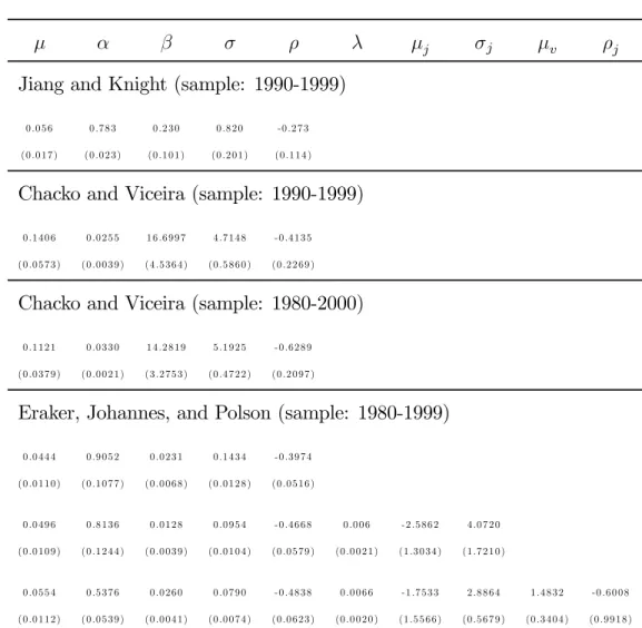
The stochastic volatility model parameter estimates are in line with those obtained in a number of recent studies that performed the estimation of stochastic volatility models on the sample of S&P 500 prices for different periods of time between years 1980 and 2000. More precisely, Jiang and Knight (2002) estimate the pure diffusion stochastic volatility model on the basis of S&P500 index daily returns for the period 1990-1999. Chacko and Viceira (2003) do the same for two samples, 1990-1999 and 1980-2000. Eraker et al. (2003) work with S&P500 returns during years 1980-1999. Table 3 contains the results of previous research. Table 2 presents our estimates for the SV, SVJ, and SVJJ models.
Insert Table 2 here. Insert Table 3 here.
At a first glance, our estimate for the µ parameter seems to be higher than the one found in the related literature and higher than the sample mean log-return of 0.05% (12.61% annualized with 252 day count). However, while others define the drift of the asset log-price directly as µ, our model specification (2) assumes µto be the drift of the asset price process. Hence, the expected asset log-return in our model is defined as (µ −1/2α), which is equal to 0.0379% for the SV model, 0.0966% for the SVJ model and0.0689% for the SVJJ process.
The long-run mean,α, of the variance process in the SV model is equal to0.5665.
This estimate is within the range of the smallest value of 0.0255 reported by Chacko
and Viceira (but remember that their parameter is annualized) the largest value of 0.9052found by Eraker et al. and is close to the0.783obtained by Jiang and Knight.
It is easy to check the plausibility of the value for this parameter by comparing it with the sample volatility, which is15.62%per annum. Our estimate leads to11.95%
average annual volatility, Eraker et al. obtain 15.10%, Jiang and Knight - 14.05%,
Chacko and Viceira -18.17%.Running ahead of the train, we would like to draw your
attention to the fact that the estimate for α of Eraker et al. will fall down to the
level of 0.5376 once they add jumps to the SV model.
The speed of mean-reversion, β, and the volatility of volatility parameter, σ,
turned out to be tedious to estimate. The range of values for β goes from 0.0231 of
Eraker et al. to16.6997of Chacko and Viceira. The volatility of volatility parameter
obtained by the same researchers is 0.1434 and5.1925respectively. Our σ is equal to
0.7813, and it is close to the parameter value of0.82 obtained by Jiang and Knight.
However, the speed of mean reversion wefind,6.3352, differs a lot from0.23of Jiang and Knight.
Such a difference in the stochastic volatility parameter estimates requires some common ground for comparison between results of various researchers. The half-life of the process is not a very indicative statistic due to the interdependence between
the speed of mean-reversion and the volatility of volatility estimates, as it has been pointed out above. However, the marginal variance of the volatility process, ασ2/2β,
involves all three parameters, and may serve our goal well. The marginal variance of the volatility process implied by our parameter estimates is 0.0273. For Chacko and
Viceira it is0.0311,Jiang and Knight -1.1445, and Eraker et al. -0.4029. As one can
see, there is no consensus again, but our results are of the same order of magnitude as Chacko and Viceira’s. To summarize, we believe further research in the area of stochastic volatility estimation may be valuable.
The correlation between the asset log-return process and the variance process is negative, in support to the stylized fact of the growing volatility in the periods of low returns, the so called leverage effect. The value of the correlation coefficient,
ρ = −0.2747, is smaller than that of Eraker et al. (−0.3974) and Chacko, Viceira (−0.6289), but it is surprisingly close to the(−0.273) estimate of Jiang and Knight.
4.4
Stochastic volatility with jumps
The inclusion of jumps in the SV model has some effect on the parameter estimates. First of all, the long-run mean of the variance process, α, drops significantly as we add jumps to the asset price process, and then to the variance. This feature is also documented by Eraker et al. (2003). Chacko and Viceira (2003) estimate a stochastic volatility model with exponential jumps in the asset prices. Even though we do not reproduce these results here, we wish to emphasize that for various jump size distributions, the value of the parameter,α,decreases with the inclusion of jumps
in the process, implying that a part of the variance of the process is induced by its discontinuous component.
The remainder of the parameters of the stochastic volatility process, namelyβ, σ
andρ,are not affected by the presence of jumps in the asset price process. Jumps in
value of the correlation coefficient, which are, however, still within the one standard deviation region of the SV model estimates. Jumps in the correlated variance process were meant to generate negative skewness of the modeled log-returns above the level which is attainable by correlated diffusions only. The inclusion of jumps in volatility in the model may reduce the correlation coefficient between the two Brownian motions due to their similar effects on the distributional characteristics of the asset log-returns. The expected size of the jump in the asset log-price of (−2.4189) is very close to the one found by Eraker et al. in the SVJ model, precisely (−2.5862). However, the variance of the jump size in our estimation as well as the intensity of the jump process are bigger than those of Eraker et al., 6.2513 vs 4.0720, and 0.0499 vs 0.006.
The explanation is that higher jump size variance allows the model to account for smaller jumps that occur more frequently.
While jumps in returns have negative mean, jumps in volatility are positive on average. This last result, combined with the negative correlation between the jump sizes, is in line with the stylized fact, called leverage effect of the stochastic volatil-ity. Our estimates for the average magnitude of jumps in the asset log-returns and jump size variance do not change significantly once the jumps in the variance process are added. Eraker et al., on the opposite, find smaller absolute mean jump size and smaller variance for the SVJJ model when compared to the SVJ model. The expla-nation is found in their expected jump in the variance process, µv = 1.4832, which is almost twice the size of our estimate of 0.8243, i.e. some distributional
characteris-tics of the asset log-returns can be equally well explained by bigger absolute value of negative jumps in the log-price and by higher expected jump in the variance process. The jump size correlation coefficient, ρj, was found to be the hardest one to estimate. As it has been pointed out before, the SVJ model is obtained from the SVJJ model by setting the variance jump sizezv = 0. Once there are no more jumps
case, as recognized by Davies (1977), the usual t-statistics is no longer distributed as normal. Notice also, that the test of zv = 0 involves a boundary. In this case, as
noticed by Chernoff(1954), the usual t-statistics does not apply.
To summarize, most of our parameter estimates for the SV model were found to be robust to the addition of jump processes to the dynamics of the state variables. The only exception is the long-run mean of the variance process that declines as jumps are added to the process. We conjecture that the continuous ECF estimator is able to pin down model parameters even if the model in not fully specified. This is a feature that requires further investigation. The comparison of the “goodness-of-fit” of the models in the framework of continuous ECF estimation for non-i.i.d. processes can be done on the basis of the value of the objective function (22) at its minimum. Even though, this does not constitute a formal test, there seems to be no alternative to test for the optimal model specification for the moment. The value of the objective function for the SV model is 23.3. For the SVJ model the objective function value is
14.8. Last, for the SVJJ model the objective function reaches a value of 13.9. Thus,
the presence of jumps in the asset prices improves significantly the fit of the model to the data. Jumps in the variance process do not have such a dramatic impact, but still provide a better fit than the SVJ model. Hence, it is essential to have at least one source of discontinuity in the asset price model. The exact specification of the continuous and discontinuous parts has a second order effect.
5
Conclusions
This paper provides the analytical solution for the unconditional joint characteristic function of the affine jump-diffusion process. The unconditional joint characteris-tic function allows us to estimate parameters of a process with unobservable state variables avoiding the discretization of the process and the simulation of the latent
variables. Three specifications of the jump-diffusion processes are estimated using the continuous empirical characteristic function method: Heston’s (1993) stochastic volatility model, a stochastic volatility model with jumps in the asset price, and a sto-chastic volatility model with jumps in both the price and the unobservable variance process.
The first goal was to further test the feasibility of the estimation procedure in itself. The second goal was to find the data-generating process that fits the best the historical distribution of the asset prices with a specific emphasis on jumps. We found that the continuous ECF procedure proved to be a good compromise between the efficiency and computational feasibility. The stochastic volatility model with jumps in both the price and the unobservable variance process has been shown tofit the data the best.
References
1. Andersen, T., Benzoni, L., and J. Lund, 2002. An empirical investigation of continuous-time equity return models. Journal of Finance, 57(3), 1239—1284. 2. Bakshi, G., Cao, C., and Z. Chen, 1997. Empirical performance of alternative
option pricing models. Journal of Finance, 52, 2003—2049.
3. Bakshi, G., Kapadia, N., and D. Madan, 2003. Stock return characteristics, skew laws, and the differential pricing of individual equity options. Review of Financial Studies,16, 101—143.
4. Bates, D., 1996. Jumps and stochastic volatility: the exchange rate processes implicit in Deutschemark options. Review of Financial Studies, 9, 69—107. 5. Bates, D., 2000. Post-’87 Crash fears in S&P 500 futures options. Journal of
Econometrics, 94, 181—238.
6. Besbeas, P., and B.J.T. Morgan, 2001. Integrated squared error estimation of Cauchy parameters. Statistics and Probability Letters, 55, 397—401.
7. Bollen, N. P. P., and R. E. Whaley, 2001. What determines the shape of implied volatility functions? Working paper.
8. Brandt, M. and P. Santa-Clara, 2002. Simulated likelihood estimation of dif-fusions with an application to exchange rate dynamics in incomplete markets.
Journal of Financial Economics, 63, 161—210.
9. Bryant, J.L., and A.S. Paulson, 1983. Estimation of mixing properties via dis-tance between characteristic functions. Communications in Statistics, Theory and Methods, 12, 1009—1029.
10. Carrasco, M., and J.P. Florens, 2000. Generalization of GMM to a continuum of moment conditions. Econometric Theory, 16, 797—834.
11. Carrasco, M., and J.P. Florens, 2002. Efficient GMM estimation using the empirical characteristic function. IDEI Working paper, n. 140.
12. Carrasco, M., Chernov, M., Florens, J.P., and E., Ghysels, 2003. Efficient estimation of jump diffusions and general dynamic models with a continuum of moment conditions. CIRANO Working Papers, 2003s—02.
13. Chacko, G., and L.M. Viceira, 2003. Spectral GMM estimation of continuous-time processes. Journal of Econometrics,116, 259—292.
14. Chernoff, H., 1954. On the distribution of the likelihood ratio. Annals of Mathematical Statistics, 25, 573—8.
15. Cox, J.C., Ingersoll Jr., J.E., and S.A. Ross, 1985. A theory of the term struc-ture of interest rates. Econometrica, 53, 385—407.
16. Csörgö, S., 1981. Limit behavior of the empirical characteristic function. Annals of probability, 9, 130—144.
17. Davies, R.B., 1977. Hypothesis testing when a nuisance parameter is present only under the alternative. Biometrika, 64(2), 247—254.
18. Duffie, D., Pan, J., and K.J. Singleton, 2000. Transform analysis and asset pricing for affine jump-diffusions. Econometrica, 68, 1343—1376.
19. Duffie, D., and K.J. Singleton, 1993. Simulated moments estimation of Markov models of asset prices. Econometrica, 61, 929—952.
20. Durham, G., and A.R. Gallant, 2002. Numerical techniques for maximum like-lihood estimation of continuous-time diffusion processes. Journal of Business
& Economic Statistics, 20(3), 297—317.
21. Eraker, B., Johannes, M., and N. Polson, 2003. The impact of jumps in volatil-ity and returns. The Journal of Finance, 58(3), 1269—1300.
22. Feller, W., 1951. Two singular diffusion problems. Annals of Mathematics,
54(1), 173—182.
23. Feuerverger, A., 1990. An efficiency result for the empirical characteristic func-tion in stafunc-tionary time-series models. The Canadian Journal of Statistics, 18, 155—161.
24. Feuerverger, A., and P. McDunnough, 1981b. On some Fourier methods for inference. Journal of the American Statistical Association, 76, 379—387.
25. Feuerverger, A., and P. McDunnough, 1981c. On the efficiency of empirical characteristic function procedures. Journal of the Royal Statistical Society, Series B, Methodological, 43, 20—27.
26. Gallant, A.R., and G. Tauchen, 1996. Which moments to match? Econometric Theory, 12, 657—681.
27. Goyal, A., and P. Santa-Clara, 2003. Idiosyncratic risk matters. Journal of Finance, 58(3), 975—1007.
28. Hansen, L., 1982. Large sample properties of generalized method of moments estimator. Econometrica, 50, 1029—1054.
29. Heathcote, C.R., 1977. The integrated squared error estimation of parameters.
Biometrika, 64, 255—264.
30. Heston, S., 1993. A closed-form solution for options with stochastic volatil-ity with applications to bond and currency options. The Review of Financial
Studies, 6,327—343.
31. Ho, M.S., Perraudin, W.R.M., and B.E. Sorensen, 1996. A Continuous-Time Arbitrage-Pricing Model with Stochastic Volatility and Jumps. Journal of Busi-ness & Economic Statistics, 14(1), 31—43.
32. Jacquier, E., Polson, N.G., and P.E. Rossi, 1994. Bayesian analysis of stochastic volatility models. Journal of Business and Economic Statistics, 12, 371—389. 33. Jiang, G.J., and J.L. Knight 2002. Estimation of continuous-time processes
via the empirical characteristic function. Journal of Business and Economic Statistics, 20(2), 198—212.
34. Jones, C.S., 1999. Bayesian estimation of continuous-time finance models. Working paper, Rochester University.
35. Knight, J.L., and S.E. Satchell, 1996. Estimation of stationary stochastic processes via the empirical characteristic function. Manuscript, Departments of Economics, University of Western Ontario.
36. Knight, J.L., and S.E. Satchell, 1997. The cumulant generating function esti-mation method. Econometric Theory, 13, 170—184.
37. Knight, J.L. and J. Yu, 2002. Empirical characteristic function in time-series estimation. Econometric Theory, 18, 691—721.
38. Kou, S., 2002. A jump-diffusion model for option pricing. Management Science, 48, 1086—1101.
39. Merton, R., 1976. Option pricing when underlying stock returns are discontin-uous. Journal of Financial Economics, 3, 125—144.
40. Newey, W.K., and K.D. West, 1994. Automatic lag selection in covariance matrix estimation. Review of Economic Studies, 61, 631—653.
41. Pan, J., 2002. The jump-risk premia implicit in options: Evidence from an integrated time-series study. Journal of Financial Economics, 63, 3—50.
42. Parzen, E., 1962. On estimation of a probability density function and mode.
Annals of Mathematical Statistics, 33, 1065—1076.
43. Paulson, A.S., Holcomb, E.W., and R.A. Leitch, 1975. The estimation of para-meters of the stable laws. Biometrika, 62, 163—170.
44. Ramezani, C.A., and Y. Zeng, 1999. Maximum likelihood estimation of asym-metric jump-diffusions process: Application to security prices. Working paper, Department of Statistics, University of Wisconsin.
45. Schmidt, P., 1982. An Improved Version of the Quandt-Ramsey MGF Estima-tor for Mixtures of Normal Distributions and Switching Regressions. Econo-metrica, 50(2), 501—524.
46. Singleton, K.J., 2001. Estimation of affine asset pricing models using the em-pirical characteristic function. Journal of Econometrics, 102, 111—141.
47. Tran, K.C., 1998. Estimating mixtures of normal distributions via empirical characteristic function. Econometric Reviews, 17, 167—83.
48. Yu, J., 2004. Empirical characteristic function estimation and its applications.
Appendix
The joint unconditional CF of the asset log-returns
This part of the appendix follows the idea of Jiang and Knight (2002).
ψ(w1,· · ·wp+1;r1,· · ·rp+1) =E " exp Ãp+1 X k=1 iwkrk !# =E " E " exp à p X k=1 iwkrk ! eiwp+1rp+1 |sp,Vp ## =E " exp à p X k=1 iwkrk ! E£eiwp+1rp+1+i0Vp+1 |sp,Vp ¤# =E " exp à p X k=1 iwkrk ! eC(1;wp+1,0)+J(1;wp+1,0)+D(1;wp+1,0)Vp # =eC(1;wp+1,0)+J(1;wp+1,0) E " exp Ãp−1 X k=1 iwkrk ! eiwprp+D(1;wp+1,0)Vp # =eC(1;wp+1,0)+J(1;wp+1,0) E " exp Ãp−1 X k=1 iwkrk ! E£eiwprp+D(1;wp+1,0)Vp |sp−1,Vp−1 ¤ # =eC(1;wp+1,0)+J(1;wp+1,0) E exp ¡Pp−1 k=1iwkrk ¢ eC(1,wp,−iD(1;wp+1,0))+J(1,wp,−iD(1;wp+1,0)) eD(1,wp,−iD(1;wp+1,0))Vp−1 = exp [C(1;wp+1,0) +C(1;wp,−iD(1;wp+1,0)) +J(1;wp+1,0) +J(1;wp,−iD(1;wp+1,0))]∗ ∗ E " E " exp Ãp−2 X k=1 iwkrk ! exp (iwp−1rp−1+D(1;wp,−iD(1;wp+1,0))Vp−1 )|sp−2,Vp−2 ## ... = exp Ãp+1 X k=1 C(1, wk, wk∗) +J(1, wk, wk∗) ! E[exp (D(1;w1, w∗1)V0)] with w∗ p+1 = 0, and w∗k=−iD ¡ 1;wk+1, w∗k+1 ¢ .
Asymptotic properties of the continuous ECF estimator
Asymptotic properties of the continuous ECF estimator, based on the findings of Feuerverger and McDunnough (1981b), Besbeas and Morgan (2001), Knight and Yu (2002), are the following. Keeping in mind that
|z|=pRe(z)2+ Im(z)2, Reϕn(u;y) = 1 n n X j cosu0yj, Imϕn(u;y) = 1 n n X j sinu0yj,
and simplifying the notation, the integral (22) can be written in the following form
In(θ) = Z · · · Z |ϕ(u;y, θ)−ϕn(u;y)| 2 g(u)du = Z · · ·Z ©[Reϕ(u;θ)−Reϕn(u)]2+ [Imϕ(u;θ)−Imϕn(u)]2ªg(u)du
and the continuous ECF estimatorˆθn is consistent,
ˆ
θn −→θ0 a.s.,
and asymptotically normally distributed
√
n(ˆθn−θ0)−→N(0, B−1(θ0)A(θ0) B−1(θ0)),
where θ0 is a true parameter vector and
B(θ0) = Z · · · Z ∂ϕ(u;θ 0) ∂θ ∂ϕ(u;θ0) ∂θ0 g(u)du = Z · · · Z · ∂Reϕ(u;θ0) ∂θ ∂Reϕ(u;θ0) ∂θ0 + ∂Imϕ(u;θ0) ∂θ ∂Imϕ(u;θ0) ∂θ0 ¸ g(u)du, A(θ) = lim n→∞ Z · · · Z ∂Reϕ(r;θ) ∂θ ∂Reϕ(u;θ) ∂θ0 ·E(θ) + 2 ∂Reϕ(r;θ) ∂θ Imϕ(u;θ) ∂θ0 ·F(θ) +∂Im∂θϕ(r;θ)∂Im∂θϕ(0u;θ) ·G(θ) g(r)g(u)drdu,
with E(θ) = 1 n n X j n X k
cov(cos(r0yj),cos(u0yk))
= 1 2{Reϕ(r+u;θ) + Reϕ(r−u;θ)}−Reϕ(r;θ) Reϕ(u;θ) + 1 2n n−1 X k=1 (n−k){ReΨk(r, u) + ReΨk(r,−u) + ReΨk(u, r) + ReΨk(u,−r)}, F(θ) = 1 n n X j n X k
cov(cos(r0yj),sin(u0yk))
= 1 2{Imϕ(r+u;θ)−Imϕ(r−u;θ)}−Reϕ(r;θ) Imϕ(u;θ) + 1 2n n−1 X k=1 (n−k){ImΨk(r, u)−ImΨk(r,−u) + ImΨk(u, r) + ImΨk(u,−r)} and G(θ) = 1 n n X j n X k
cov(sin(r0yj),sin(u0yk))
= 1 2{Reϕ(r−u;θ)−Reϕ(r+u;θ)}−Imϕ(r;θ) Imϕ(u;θ) + 1 2n n−1 X k=1 (n−k){ReΨk(r,−u)−ReΨk(r, u) + ReΨk(u,−r)−ReΨk(u, r)} where Ψk(r, u) =E[exp (ir0y1+iu0yk+1)].
B(θ0)andA(θ0)can be consistently estimated: B(θ0)byB(ˆθn)andA(θ0)by applying
Captions
Table 1 contains descriptive statistics for the S&P500 index daily log-returns. The sample covers the period between January 2nd 1980 and December 31st 1999. The returns are expressed in percent.
Table 2 presents parameter estimates for the three models: SV, SVJ, and SVJJ. The sample is the one described above. Note, that the estimates are daily parameters for return process expressed in percent. The estimation was done using the continuous ECF estimator with a block sizep+1 = 2and a normal weight function. The variance
of the weight function was set to be equal to 1.5.
Table 3 consists of parameter estimates obtained by the previous researchers. The results of Jiang and Knight (2002) correspond to the pure diffusion stochastic volatility model estimated on the basis of S&P500 index daily returns for the period 1990-1999 using the unconditional joint ECF estimation procedure with the block size equal to 2. The estimates are daily parameters for return process expressed in percent. The estimates of Chacko and Viceira (2003) presented here are for the pure diffusion stochastic volatility model. They are obtained by applying the Spectral GMM to the S&P500 index prices between years 1980 and 2000. The parameter estimates are annualized and expressed in the decimal points. Eraker, Johannes and Polson (2003) estimates related to this work are the ones for the SV, SVJ and SVJJ models for the S&P500 daily returns between years 1980-1999. Again, estimates are daily parameters for return process expressed in percent.
Figure 1plots time series of the S&P500 index daily log-returns. Horizontal lines are+/−3standard deviations around the mean of the S&P500 log-return distribution. One notices the presence of sudden, non-persistent changes in the returns.
Table 1. Descriptive statistics
for the S&P 500 daily log-returns expressed in percent.
mean standard deviation min max skewness kurtosis 0.050037 0.9839 -22.8330 8.7089 -2.6455 64.2380
Table 2. Parameter estimates for the jump-diffusion models
using S&P 500 daily log-returns expressed in percent
µ α β σ ρ λ µj σj µv ρj In(θ) SV 0 .3 2 1 2 0 .5 6 6 5 6 .3 3 5 2 0 .7 8 1 3 -0 .2 7 4 7 2 3 .3 (0 .0 1 4 ) (0 .0 1 2 ) (0 .2 1 0 ) (0 .1 8 6 ) (0 .1 7 9 ) SVJ 0 .3 4 7 0 0 .5 0 0 7 6 .3 2 9 4 0 .7 9 2 1 -0 .2 7 6 5 0 .0 4 9 9 -2 .4 1 8 6 6 .2 5 1 3 1 4 .8 (0 .1 1 1 ) (0 .0 1 2 ) (0 .2 1 3 ) (0 .2 1 3 ) (0 .1 8 8 ) (0 .0 1 2 ) (0 .9 0 2 ) (0 .9 3 6 ) SVJJ 0 .3 1 6 4 0 .4 9 5 1 6 .1 1 6 4 0 .7 9 6 9 -0 .2 6 0 7 0 .0 4 8 7 -2 .3 3 3 1 6 .3 6 7 9 0 .8 2 4 3 -0 .5 5 1 5 1 3 .9 (0 .0 9 2 ) (0 .0 1 3 ) (0 .2 5 6 ) (0 .2 4 6 ) (0 .1 9 7 ) (0 .0 0 4 ) (0 .8 8 3 ) (0 .8 7 7 ) (0 .8 9 0 ) (0 .8 9 1 )
Table 3. Parameter estimates of previous researchers
forS&P 500 daily log-returns expressed in percent
µ α β σ ρ λ µj σj µv ρj
Jiang and Knight (sample: 1990-1999)
0 .0 5 6 0 .7 8 3 0 .2 3 0 0 .8 2 0 -0 .2 7 3
(0 .0 1 7 ) (0 .0 2 3 ) (0 .1 0 1 ) (0 .2 0 1 ) (0 .1 1 4 )
Chacko and Viceira (sample: 1990-1999)
0 .1 4 0 6 0 .0 2 5 5 1 6 .6 9 9 7 4 .7 1 4 8 -0 .4 1 3 5
(0 .0 5 7 3 ) (0 .0 0 3 9 ) (4 .5 3 6 4 ) (0 .5 8 6 0 ) (0 .2 2 6 9 )
Chacko and Viceira (sample: 1980-2000)
0 .1 1 2 1 0 .0 3 3 0 1 4 .2 8 1 9 5 .1 9 2 5 -0 .6 2 8 9
(0 .0 3 7 9 ) (0 .0 0 2 1 ) (3 .2 7 5 3 ) (0 .4 7 2 2 ) (0 .2 0 9 7 )
Eraker, Johannes, and Polson (sample: 1980-1999)
0 .0 4 4 4 0 .9 0 5 2 0 .0 2 3 1 0 .1 4 3 4 -0 .3 9 7 4 (0 .0 1 1 0 ) (0 .1 0 7 7 ) (0 .0 0 6 8 ) (0 .0 1 2 8 ) (0 .0 5 1 6 ) 0 .0 4 9 6 0 .8 1 3 6 0 .0 1 2 8 0 .0 9 5 4 -0 .4 6 6 8 0 .0 0 6 -2 .5 8 6 2 4 .0 7 2 0 (0 .0 1 0 9 ) (0 .1 2 4 4 ) (0 .0 0 3 9 ) (0 .0 1 0 4 ) (0 .0 5 7 9 ) (0 .0 0 2 1 ) (1 .3 0 3 4 ) (1 .7 2 1 0 ) 0 .0 5 5 4 0 .5 3 7 6 0 .0 2 6 0 0 .0 7 9 0 -0 .4 8 3 8 0 .0 0 6 6 -1 .7 5 3 3 2 .8 8 6 4 1 .4 8 3 2 -0 .6 0 0 8 (0 .0 1 1 2 ) (0 .0 5 3 9 ) (0 .0 0 4 1 ) (0 .0 0 7 4 ) (0 .0 6 2 3 ) (0 .0 0 2 0 ) (1 .5 5 6 6 ) (0 .5 6 7 9 ) (0 .3 4 0 4 ) (0 .9 9 1 8 )
Figure 1:
The FAME Research Paper Series
The International Center for Financial Asset Management and Engineering (FAME) is a private foundation created
in 1996 on the initiative of 21 leading partners of the finance and technology community, togeth er with three
Universities of the Lake Geneva Region (Switzerland). FAME is about Research, Doctoral Training, and Executive
Education with “interfacing” activities such as the FAME lectures, the Research Day/Annual Meeting, and the Research Paper Series.
The FAME Research Paper Series includes three types of contributions: First, it reports on the research carried out at FAME by students and research fellows; second, it includes research work contributed by Swiss academics and practitioners interested in a wider dissemination of their ideas, in practitioners' circles in particular; finally, prominent international contributions of particular interest to our constituency are included on a regular basis. Papers with strong practical implications are preceded by an Executive Summary, explaining in non-technical terms the question asked, discussing its relevance and outlining the answer provided.
Martin Hoesli is acting Head of the Research Paper Series. Please email any comments or queries to the following
address: [email protected].
The following is a list of the 10 most recent FAME Research Papers. For a complete list, please visit our website at www.fame.ch under the heading ‘Faculty and Research, Research Paper Series, Complete List’.
N°149 Suggested vs Actual Institutional Allocation to Real Estate in Europe: A Matter of Size?
Martin HOESLI, University of Geneva and FAME and University of Aberdeen; Jon LEKANDER, Aberdeen Property Investors, Stockholm
N°148 Monte Carlo Simulations for Real Estate Valuation
Martin HOESLI, HEC Geneva and FAME and University of Aberdeen; Elion JANIi, HEC Geneva, André BENDER, HEC Geneva and FAME
N°147 Equity and Neutrality in Housing Taxation
Philippe THALMANN, Ecole Polytechnique Fédérale de Lausanne
N°146 Order Submission Strategies and Information: Empirical Evidence from NYSE
Alessandro BEBER, HEC Lausanne and FAME; Cecilia CAGLIO, U.S. Security and Exchange Commission
N°145 Kernel Based Goodness-of-Fit Tests for Copulas with Fixed Smoothing Parameters
Olivier SCAILLET, HEC Geneva and FAME
N°144 Multivariate wavelet-based shape preserving estimation for dependent observations
Antonio COSMA, Instituto di Finanza, University of Lugano, Lugano, Olivier SCAILLET, HEC Geneva and FAME, Geneva, Rainier von SACHS, Institut de statistiq ue, Université catholique de Louvain
N°143 A Kolmogorov-Smirnov type test for shortfall dominance against parametric alternatives
Michel DENUIT, Universitéde Louvain, Anne-Cécile GODERNIAUX, Haute Ecole Blaise Pascal Virton, Olivier SCAILLET, HEC, University of Geneva and FAME
N°142 Times-to-Default: Life Cycle, Global and Industry Cycle Impacts
Fabien COUDREC, University of Geneva and FAME, Olivier RENAULT, FERC, Warwick Business School
N°141 Understanding Default Risk Through Nonparametric Intensity Estimation
Fabien COUDREC, University of Geneva and FAME
N°140 Robust Mean-Variance Portfolio Selection