Title
Testing the predictive ability of technical analysis using a new
stepwise test without data snooping bias
Author(s)
Hsu, PH; Hsu, YC; Kuan, CM
Citation
Journal Of Empirical Finance, 2010, v. 17 n. 3, p. 471-484
Issued Date
2010
URL
http://hdl.handle.net/10722/141768
Testing the Predictive Ability of Technical Analysis Using
A New Stepwise Test without Data Snooping Bias
Po-Hsuan Hsu
Department of Finance University of Connecticut
Yu-Chin Hsu
Department of Economics University of Texas at Austin
Chung-Ming Kuan
Department of Finance National Taiwan University
This version: July 20, 2009
†Author for correspondence: Po-Hsuan Hsu, [email protected]
††We thank the editor, Christian C. P. Wolff, and two anonymous referees for their useful comments and
suggestions. We are grateful for the comments on early versions of this paper by Zongwu Cai, Stephen Donald, Peter R. Hansen, Joel Hasbrouck, Shantaram Hegde, Yingyao Hu, Robert Lieli, Chris Neely, Pedro Saffi, Michael Wolf, Yangru Wu, and Jialin Yu. We also thank the participants of the Inaugural Conference of the Society for Financial Econometrics, Financial Management Association Meeting, North American Summer Meeting of the Econometric Society, NTU IEFA Conference, and the seminars in Columbia University, National Central University, National Taiwan University, National University of Singapore, University of North Carolina at Charlotte, and University of Rochester. P.-H. Hsu is especially indebted to Andrew Ang, Charles M. Jones, and John Donaldson for their guidance during his doctoral study at the Graduate School of Business of Columbia University. C.-M. Kuan thanks the NSC of Taiwan for research support (97–2410–H–002–217–MY3). All errors remain ours.
Testing the Predictive Ability of Technical Analysis Using
A New Stepwise Test without Data Snooping Bias
Abstract
In the finance literature, statistical inferences for large-scale testing problems usually suffer from data snooping bias. In this paper we extend the “superior predictive ability”
(SPA) test of Hansen (2005, JBES) to a stepwise SPA test that can identify predictive
models without potential data snooping bias. It is shown analytically and by simulations that the stepwise SPA test is more powerful than the stepwise Reality Check test of
Romano and Wolf (2005, Econometrica). We then apply the proposed test to examine
the predictive ability of technical trading rules based on the data of growth and emerging market indices and their exchange traded funds (ETFs). It is found that technical trading rules have significant predictive power for these markets, yet such evidence weakens after the ETFs are introduced.
JEL classification: C12, C32, C52, G11
Keywords: data snooping, exchange traded funds, reality check, SPA test, stepwise test, technical trading rules
1
Introduction
Technical analysis has been widely applied in stock markets since W. P. Hamilton wrote
a series of articles inThe Wall Street Journalin 1902. Its predictive power (or
profitabil-ity), however, remains a long-debated issue in both industry and academia. A recent
article in The Wall Street Journal observes: “Some brokerage firms have eliminated
their technical research departments altogether. Still, when the markets begin to sag, in-vestors rediscover technical analysis” (Browning, July 30, 2007). Indeed, the same article reports that some technical analysts did foresee and warn their clients right before the stock market plunge on July 23, 2007. There are also numerous empirical results in the literature that support technical analysis, such as Sweeney (1988), Blume, Easley, and O’Hara (1994), Brown, Goetzmann, and Kumar (1998), Gencay (1998), Lo, Mamaysky, and Wang (2000), and Savin, Weller, and Zvingelis (2007). Such evidences, however, may be criticized for their data snooping bias; see, e.g., Lo and MacKinlay (1990) and Brock, Lakonishok, and LeBaron (1992).
Data snooping is common in the finance and economics literature. In practice, only a few financial data sets are available for empirical examination. Data snooping arises when researchers rely on the same data set to test the significance of different models (technical trading rules) individually. As these individual statistics are generated from the same data set and hence related to each other, it is difficult to construct a proper joint test, especially when the number of models (rules) being tested is large. White (2000) proposes a large-scale joint testing method for data snooping, also known as Reality Check (RC), which takes into account the dependence of individual statistics. Sullivan, Timmermann, and White (1999) apply the RC test and find that technical trading rules lose their predictive power for major U.S. stock indices after the mid 80’s.
White’s RC test suffers from two drawbacks. First, Hansen (2005) points out that the RC test is conservative because its null distribution is obtained under the least favorable configuration, i.e., the configuration that is least favorable to the alternative. In fact, the RC test may lose power dramatically when many poor models are included in the same test. To improve on the power property of the RC test, Hansen (2005) proposes the “superior predictive ability” (SPA) test that avoids the least favorable configuration. Empirical studies, such as Hansen and Lunde (2005) and Hsu and Kuan (2005), also show
that the SPA test is more powerful than the RC test. Second, the RC test checks whether there is any significant model but does not identify all such models. Note that Hansen’s SPA test shares the same limitation. Romano and Wolf (2005) introduce a RC-based stepwise test, henceforth Step-RC test, that is capable of identifying as many significant models as possible. Nonetheless, Romano and Wolf’s Step-RC test is conservative because its stepwise critical values are still determined by the least favorable configuration, as in the original RC test.
In this paper, the SPA test is further extended to a stepwise SPA (Step-SPA) test that can identify predictive models in large-scale, multiple testing problems without data snooping bias. This is analogous to the extension of White’s RC test to Romano and Wolf’s Step-RC test. It is shown that the Step-SPA test is consistent, in the sense that it can identify the violated null hypotheses (models or rules) with probability approaching one, and its familywise error (FWE) rate can be asymptotically controlled at any pre-specified level, where FWE rate is defined as the probability of rejecting at least one correct null hypothesis. This paper makes additional contribution by showing analytically and by simulations that the Step-SPA test is more powerful than the Step-RC test, under any power criterion defined in Romano and Wolf (2005).
In our empirical study, the proposed Step-SPA test is applied to evaluate the pre-dictive power of 9,120 moving average rules and 7,260 filter rules in several growth and emerging markets. Unlike many existing studies on technical analysis, we examine not only market indices but also their corresponding Exchange Traded Funds (ETFs). Con-sidering ETFs is practically relevant because ETFs have been important investment vehicles since their inception in late 90’s. Moreover, due to the tradability and low transaction costs, ETFs help to increase market liquidity and hence may improve market efficiency (e.g. Hegde and McDermott, 2004). Our empirical study thus enables us to assess whether the predictive power of technical rules, if any, is affected after ETFs are introduced.
Our empirical results provide strong evidence that technical rules have significant predictive ability in pre-ETF periods, yet such evidence weakens in post-ETF periods. In particular, we find many technical rules with significant predictive power prior to the
market indices become available. For emerging markets, we find technical rules have predictive ability for 4 (out of 6) index returns but for only 2 ETF returns. For these two predictable ETFs, far fewer rules with significant predictive power can be identified by the proposed stepwise test. The high break-even transaction costs associated with the top rules in those predictable ETFs further suggest that some technical rules may be exploited to make profit in certain emerging markets. Our findings therefore indicate a negative impact of the inception of ETFs on the predictive ability of technical trading rules. This is compatible with the intuition that ETFs allow arbitrageurs to trade away most potential profits in young markets.
To summarize, this paper makes the following contributions to the literature. First, we develop a new test for empirical testing problems in finance that require correction of data snooping bias. Second, we provide new evidence of technical predictability (and potential profitability) of growth and emerging stock markets based on recently available data of ETFs. Last, but not least, this study supports the adaptive market efficiency hy-pothesis of Lo (2004). Using technical predictability as a barometer of market efficiency,
our results suggest that the existence of ETFs effectively improves market efficiency.1
This paper proceeds as follows. We summarize the existing tests and introduce the Step-SPA test in Section 2. The simulation results for the Step-SPA test are reported in Section 3. The data and performance measures are discussed in Section 4. The empirical results are presented in Section 5. Section 6 concludes the paper. The proofs and some details of the technical rules considered in the paper are deferred to Appendices.
2
Tests without Data Snooping Bias
Givenm models for some variable, letdk,t (k= 1,2, ..., mandt= 1,2, ..., n) denote their
performance measures (relative to a benchmark model) over time. Suppose that for each
k, IE(dk,t) = µk for all t, and for each t, dk,t may be dependent across k. We wish to
determine whether these models can outperform the benchmark and would like to test the following inequality constraints:
H0k :µk ≤0, k= 1, ..., m. (1)
1Neely, Weller, and Ulrich (2007) also suggest that the weakening technical predictability in foreign
For example, we may test if there is any technical trading rule that can generate positive
return for an asset. Letrt be the return of this asset at timetand δk,t−1 be the trading
signal generated by thek-th trading rule at timet−1, which takes the values of 1, 0, or−1,
corresponding to a long position, no position, and a short position, respectively. Then,
dk,t = δk,t−1rt is the realized return of the k-th trading rule, and (1) is the hypothesis
that notrading rule can generate positive mean return. Note that dk,t depend on each
other because they are based on the same returnrt.
Following Hansen (2005), we impose the following condition on dt = (d1,t, ..., dm,t)0
which allowsdt to exhibit weak dependence over time.
Assumption 2.1 {dt}is strictly stationary andα-mixing of size−(2 +η)(r+η)/(r−2),
for some r > 2 and η > 0, where E|dt|(r+η) < ∞ with | · | the Euclidean norm, and
var(dk,t)>0 for allk.
Under this condition, the data obey a central limit theorem: √
n(¯d−µ)−→ ND (0,Ω), (2)
where ¯d =n−1Pn
t=1dt, µ= IE(dt), Ω≡ limn→∞var(
√
n(¯d−µ)), and −→D stands for convergence in distribution. Moreover, Assumption 2.1 ensures the validity of the sta-tionary bootstrapping procedure and the consistency of the covariance matrix estimator of Politis and Romano (1994).
2.1 Existing Tests
Data snooping arises when the inference for (1) is drawn from the test of an individual
hypothesisHk
0. One may circumvent the problem by controlling the significance level of
each individual test based on the Bonferroni inequality. This approach is, however, not
practically useful when the number of hypotheses, m, is large. In many applications,
m is typically very large; for example, Sullivan et al. (1999) evaluate 7,846 technical
trading rules, and Hsu and Kuan (2005) study a total of 39,832 simple technical rules and complex trading strategies.
Alternatively, one may conduct a joint test of (1) with a properly controlled signifi-cance level. A leading example is the RC test of White (2000) with the statistic:
RCn= max
k=1,...,m
√
where ¯dkis thek-th element of ¯d. Given that (1) is a collection of composite hypothesis,
White (2000) chooses the least favorable configuration (LFC), i.e.,µ=0, to obtain the
null distribution. It follows from (2) that√nd¯ −→ ND (0,Ω) under the LFC. The limiting
distribution of RCnis thus max{N(0,Ω)}which may be approximated via a (stationary)
bootstrap procedure. The null hypothesis (1) would be rejected when the bootstrapped
p-value is smaller than a pre-specified significance level or, equivalently, when the test
statistic RCn is greater than the bootstrapped critical value.
The LFC of the RC test is convenient but also renders this test relatively conservative.
Hansen (2005) shows that under the null, when there are someµi <0 and at least one
µi = 0, RCn −→D max{N(0,Ω0)}, where Ω0 is a sub-matrix of Ω with the j-th row
and j-th column of Ω deleted when µj <0. That is, the limiting distribution depends
only on the models with a zero mean but not on those poor models (i.e., the models
with a negative mean). It is also conceivable that including very poor models may
artificially increase the empiricalp-value of the RC test. This motivates the SPA test of
Hansen (2005) with the statistic:
SPAn= max max k=1,...,m √ nd¯k, 0 ,
which is virtually the same as the RC test.
A novel feature of the SPA test is that it avoids the LFC by re-centering the null
distribution, as described below. Let Ωb denote a consistent estimator for Ω with the
(i, j)-th element ˆωij. Also let ˆσk2 ≡ωˆkk and An,k=−σˆk√2 log logn. We define ˆµas the
vector with thek-th element:
ˆ
µk = ¯dk1 √nd¯k≤An,k,
where 1(B) denotes the indicator function of the event B. It can be seen that ˆµk = 0
almost surely when µk = 0. Moreover, when µk < 0, √nd¯k ≤ An,k with probability
approaching one, so that ˆµk converges in probability toµk. Noting that√nd¯ =√n(¯d−
µ) + √nµ, Hansen (2005) suggests to add √nµˆ to the bootstrapped distribution of √
n(¯d−µ). Re-centering the bootstrapped distribution thus yields a better approximation
to the null distribution of SPAn: max{N(0,Ω0),0}. The SPA test is a more powerful test
than the RC test because the bootstrapped SPAp-value is smaller than the corresponding
Another drawback of the RC test is that it does not identify all models that signif-icantly deviate from the null hypothesis. Rejecting the null hypothesis by the RC test
only suggests that there exists at least one model with µk >0. Basing on the RC test,
Romano and Wolf (2005) propose a stepwise procedure that can identify as many models
withµk>0 as possible, while asymptotically controlling the FWE rate, the probability
of rejecting at least one of the correct hypotheses. This test, also known as the Step-RC test, is practically more useful than the RC test. For example, a fund-of-fund manager ought to be more interested in finding out the funds that can beat the benchmark, rather than just knowing the best performed fund.
To implement the stepwise procedure, we re-arrange ¯dk in a descending order. A top
modelkwould be rejected if√nd¯kis greater than the bootstrapped critical value, where
bootstrapping is computed as in the RC test. If none of the null hypotheses is rejected,
the process stops; otherwise, we remove ¯dk of the rejected models from the data and
bootstrap the critical value again using the remaining data. In the new sample, a top
modeliwould be rejected if√nd¯iare greater than the newly bootstrapped critical value.
The procedure continues until no more model can be rejected. Note that Hansen (2005)
and Romano and Wolf (2005) also suggest that using studentized statistics, √nd¯k/σˆk,
would render the test more powerful. To ease the expression, our discussion below is still based on non-studentized statistics.
2.2 The Stepwise SPA Test
Analogous to the extension from the RC test to the Step-RC test, it is natural to extend the SPA test to the Step-SPA test. The stepwise procedure enables us to identify signif-icant models, as in the Step-RC test, yet it ought to be more powerful because its null distribution does not depend on the LFC. The proposed Step-SPA test is based on the
following statistics: √nd¯1, . . . ,√nd¯m, and a stepwise procedure analogous to that of the
Step-RC test.
For the Step-SPA test, we adopt the stationary bootstrap of Politis and Romano (1994)
which is computed as follows. Letd∗t(b) ≡ d∗nb,t, t = 1, . . . , n, be the b-th re-sample of
dt, where the indicesnb,1, ..., nb,n consist of blocks of {1, ..., n} with random lengths
First,nb,1 is randomly chosen from{1, ..., n} with an equal probability assigned to each
number. Second, for any t > 1,nb,t =nb,t−1+ 1 with probability Q;2 otherwise, nb,t is
chosen randomly from {1, ..., n}. A re-sample is done when n observations are drawn;
let ¯d∗(b) = Pn
t=1d
∗
t(b)/n denote the sample average of this re-sample. Repeating this
procedureB times yields an empirical distribution of ¯d∗ with B realizations. Given the
pre-specified levelα0, the bootstrapped SPA critical value is determined as
ˆ
q∗α0 = max(ˆqα0, 0), (3)
with ˆqα0 = inf
q | P∗[√nmaxk=1,...,m( ¯d∗k−d¯k+ ˆµk) ≤ q] ≥ 1−α0 , the (1−α0)-th
quantile of the re-centered empirical distribution, andP∗ is the bootstrapped probability
measure.
The Step-SPA test with the pre-specified levelα0 then proceeds as follows.
1. Re-arrange ¯dk in a descending order.
2. Reject the top model k if √nd¯k is greater than ˆqα∗0(all), the critical value
boot-strapped as in (3) using the complete sample. If no model can be rejected, the procedure stops; otherwise, go to next step.
3. Remove ¯dk of the rejected models from the data. Reject the top model i in the
sub-sample of remaining observations if √nd¯i is greater than ˆqα∗0(sub), the critical
value bootstrapped as in (3) from the sub-sample. If no model can be rejected, the procedure stops; otherwise, go to next step.
4. Repeat the third step till no model can be rejected.
When the critical values in the procedure above are bootstrapped as in the RC test, we obtain a version of Step-RC test, which is in the spirit of Romano and Wolf (2005) but
implemented differently.3
2
Ifnb,t−1=n, we use the wrap-up procedure and setnb,t= 1.
3The original Step-RC test of Romano and Wolf (2005) differs from our procedure in the following
ways. First, they use circular block bootstrap, rather than stationary bootstrap. Second, they rely on a
data-dependent algorithm to determine the block size of bootstrap, rather than using anex antefixed
value. Third, they use bootstrapped standard errors, rather than heteroskedasticity and autocorrelation consistent (HAC) estimators based on sample data; see also footnote 5. These differences may affect the finite sample performance of the Step-RC test.
The results below show that the Step-SPA test is consistent while asymptotically controlling the FWE rate at a pre-specified level, analogous to Theorem 4.1 of Romano and Wolf (2005). All proofs of theorems are collected in Appendix A.
Theorem 2.2 The following results hold under Assumption 2.1 and α0 <1/2.
1. The hypothesisH0kwithµk>0 will be rejected by the Step-SPA test with probability
approaching 1 when n tends to infinity.
2. Given the pre-specified level α0, the FWE rate of the Step-SPA test is α0 when n
tends to infinity if and only if there is at least one µk= 0.
Note that the FWE rate of the Step-RC test is less than or equal toα0, in contrast with
the second result above. This is due to the fact that the RC test relies on the LFC and
hence yields a conservative test. If there is no µk = 0, it can also be shown that the
FWE rate is zero asymptotically,4 so that no null hypothesis will be incorrectly rejected.
As far as power is concerned, our key result below shows that the Step-SPA test is superior than the Step-RC test.
Theorem 2.3 Given Assumption 2.1, the SPA test is more powerful than the Step-RC test under the notions of power defined in Romano and Wolf (2005).
3
Simulations
In this section, we evaluate the finite-sample performance of the Step-SPA and Step-RC tests using Monte Carlo simulations. We are mainly concerned with the FWE rate and the rejection frequency of the models with significant returns. This is similar to the examination of the empirical level and power of a test.
We first generatem return series:
xi,t =ci+γxi,t−1+i,t, i= 1, . . . , m, t= 1, . . . , T
4
Whenµk<0, √
nd¯kwould diverge to negative infinity in probability. Given that the critical value is
always non-negative,Hk0 would be rejected with probability approaching zero, which implies that FWE
wherei,t are i.i.d. noises distributed as N(0, σ2), ci and γ are parameters such that ci
is a constant a for i = 1, . . . , m1, ci = 0 for i = m1 + 1, . . . , m1+m2, and ci = −a
for i = m1 +m2 + 1, . . . , m. We first set a = 0.0008 (8 basis points), γ = 0.01, and
σ= 0.005. Thus, each sample containsm1 “outperforming” returns that have a positive
mean 0.0008/0.99 = 0.00081, m2 “neutral” returns with a zero mean, andm−m1−m2
“poor” returns with a negative mean−0.00081. The numbers of return series arem= 90,
900 and 9000, the sample size isn= 1000, and the number of simulation replications is
R= 500. For eachm, there are three cases: (1)m1 =m2=m/3 so that there are 3 equal
groups of returns, (2)m1 =m2 =m/9 so that there are unequal groups of returns with
a much larger group of “poor” returns, and (3) m2 = m so that there are only neutral
returns. In the stationary bootstrap, we set the number of bootstrapsB = 500 and the
parameter of the geometric distributionQ= 0.9. To estimate the covariance matrix Ω0,
we use the consistent estimator of Politis and Romano (1994) in the simulations and
subsequent empirical study.5
The simulation results based on non-studentized and studentized statistics are
sum-marized in Tables 1 and 2, respectively. Here, ¯dk = ¯xk, the sample average of the k-th
return series. For Table 1, thek-th return would be rejected if√nx¯k is greater than the
5% bootstrapped critical value. For Table 2, we base the test decisions on studentized
statistics√nx¯k/σˆk, where ˆσk is as discussed in Section 2.1 and computed from the
sam-ple data.6 In each replication, the rejection rate of these tests is the number of correctly
rejected returns divided bym1, the total number of outperforming returns. Averaging
these rejection rates overR, the number of replications, yields the average rejection (AR)
5
Following Hansen (2005), the following estimator due to Politis and Romano (1994) is used: ˆ Ω = ˆΩ0+ n−1 X j=1 κ(j, n)[ ˆΩj+ ˆΩ0j],
where ˆΩj=n−1Pnt=j+1(dt−d¯)(dt−j−d¯)0 and the weight functionκ(j, n) is defined as
κ(j, n)≡ n−j n (1−Q) j + j n(1−Q) n−j ,
whereQis the parameter of the geometric distribution. This HAC estimator is similar to that of Newey
and West (1987) but with a different weight function.
6
For the studentized method, the bootstrapped statistics are computed as √nx¯∗k/σˆk,k = 1, . . . , m.
That is, ˆσk from the sample data is also used in bootstrap. One could also compute the bootstrapped
statistics as√nx¯∗k/σˆ ∗ k, with ˆσ
∗
rate, which is also the “average power” defined in Romano and Wolf (2005). The FWE rate is computed as the relative frequency of the replications in which at least one neutral or poor return is incorrectly rejected. In Tables 1 and 2 we report the average rejection rates in the first step, the average rejection rates in all steps, and the FWE rates of the Step-SPA and Step-RC tests. Note that case 3 contains only the FWE rates, because
there is no outperforming return (m1= 0).
Table 1 shows that, for the first two cases, the FWE rates of the Step-SPA test are controlled properly and closer to the nominal level 5% than those of the Stpe-RC test. Note that case 3 is exactly the LFC considered by the RC test. Thus, it is not surprising to see that the Step-SPA and Step-RC tests have the same FWE rates in this case (the last column of Table 1) becasue the Step-SPA test has no advantage here. Moreover, we
find that the FWE rate of the Step-SPA test is much smaller than 5% whenm is large,
but it is closer to 5% whenm= 90. This shows that the second result of Theorem 2.2 is
relevant in finite samples whenm is small relative to the sample sizen. Whenm is too
large, the test becomes more conservative.
Moreover, we can see that the Step-SPA test is more powerful than the Step-RC test
in terms of average rejection rate. For each m, the improvement of the Step-SPA test
over the Step-RC test is greater when there are unequal groups of returns (with a larger
number of poor models). Such improvement becomes more significant when m is large.
The greatest improvement is about 16% (81.4% for the Step-SPA test vs. 65.4% for the
Step-RC test) which occurs form= 9000 with unequal groups of returns. All the results
support the argument of Hansen (2005) that the RC test is adversely affected by the number of poor models included in the test. It is also clear that the stepwise procedure does identify more significant returns than its one-step counterpart. Yet, the power gain is
quite marginal for the Step-RC test. For example, whenm= 900 with unequal groups of
returns, further steps of the Step-SPA test identify 2.3% more significant returns (91.9% vs. 94.2%), whereas the Step-RC test only finds extra 0.6% significant returns (83.8% vs. 84.4%).
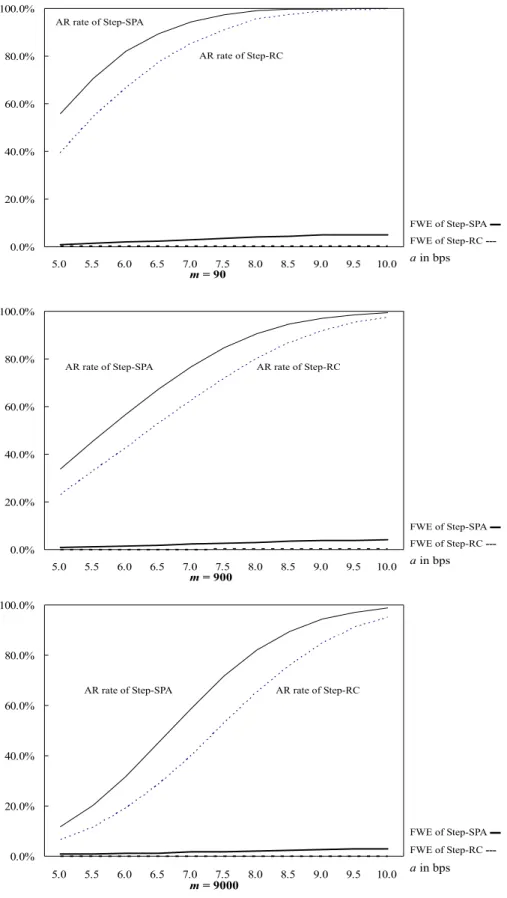
From Table 2 it is readily seen that the Step-SPA and Step-RC tests are marginally improved when studentized statistics are used and that all the conclusions based on Table 1 carry over. We also note that these simulation results are quite robust to different
a values for ci. In Figure 1, we plot the average rejection rates and FWE rates for
a= 0.0005,0.00055, . . . ,0.001 andm= 90, 900, and 9000 with unequal groups of returns.
We can see that the rejection frequencies and FWE rates increase witha; that is, these
tests reject the null more easily when the return has a larger mean. More importantly,
the Step-SPA test uniformly dominates the Step-RC test acrossavalues in all 3 panels of
Figure 1. Similar findings are obtained in unreported simulations with various settings,
such as correlated i and different γ. All the results support the theoretical properties
established in Section 2.2 and unambiguously indicate that the Step-SPA test ought to be preferred to the Step-RC test in practice.
4
Empirical Data and Performance Measures
In our empirical study, we evaluate the predictive ability of technical trading rules based on the data of market indices and corresponding ETFs. When an index is found to be predictable, one may question whether it can be easily traded by (U.S.) investors. This concern is practically relevant, especially for the indices of emerging markets, but it can be mitigated to a large extent when ETFs are available. Indeed, ETFs have been powerful investment tools for arbitrageurs and hedge funds because they track market indices closely and can be conveniently traded at low transaction costs. Thus, it makes practical sense to also examine the predictability of ETFs.
4.1 Index and ETF Data
We consider three indices of U.S. growth markets: S&P SmallCap 600/Citigroup Growth Index (SP600SG), Russell 2000 Index (RUT2000), and NASDAQ Composite Index (NAS-DAQ), and the ETFs that track these indices: SmallCap 600 Growth Index Fund (IJT), Russell 2000 Index Fund (IWM), and NASDAQ Composite Index Tracking Fund (ONEQ). We also consider the indices of six emerging markets, including MSCI Emerging Mar-kets Index, MSCI Brazil Index, MSCI South Korea Index, MSCI Malaysia Index, MSCI
Mexico Index, and MSCI Taiwan Index.7 The corresponding ETFs are: MSCI Emerging
7
Note that the MSCI indices are evaluated in U.S. dollars and reflect the holding returns on these markets for U.S. investors. These MSCI indices are important references to institutional investors, and they mitigate the liquidity and tradability issues in emerging markets because they include only investable larger stocks (Chang, Lima, and Tabak, 2004).
Markets Index Fund (EEM), MSCI Brazil Index Fund (EWZ), MSCI South Korea Index Fund (EWY), MSCI Malaysia Index Fund (EWM), MSCI Mexico Index Fund (EWW), and MSCI Taiwan Index Fund (EWT). All ETFs are issued by iShares, except that NASDAQ Composite Index Tracking Fund is issued by Fidelity.
The SP600SG and all MSCI indices are taken from Global Insight, while the other two U.S. indices and all ETFs are taken from Yahoo Finance with dividend adjustment. These data are partitioned into pre- and post-ETF periods, i.e., the periods before and after the inception of the corresponding ETF. Table 3 summarizes the pre-ETF periods for all indices (upper panel), the post-ETF periods for all ETFs up to the end of the year 2005 (lower panel), and the inception dates of the ETFs. All pre-ETF periods have more than 2,000 observations, yet the numbers of observations in post-ETF periods are quite different. For example, MSCI Malaysia and Mexico Index Funds have more than 2,000 observations, but NASDAQ Composite Index Tracking Fund and MSCI Emerging Markets Index Fund have only 508 and 566 observations, respectively.
Table 4 contains the descriptive statistics of daily holding returns on the indices and ETFs considered in the paper. We can see that, for U.S. markets, NASDAQ Composite
Index yields the highest daily return (7.4 basis points) and the largest standard deviation
in the pre-ETF period, but its ETF has the smallest mean and standard deviation in the post-ETF period. For emerging markets, MSCI Mexico Index enjoys the largest
mean return of 12.5 basis points in the pre-ETF period, and the MSCI South Korea
Index Fund has the largest mean return of 9.3 basis points in the post-ETF period. The
Ljung-BoxQstatistics indicate that, at 5% level, all index returns have significant
first-order autocorrelations, and all ETFs but MSCI Taiwan Index Fund have insignificant autocorrelations. Moreover, all index and ETF returns are leptokurtic; in particular, the index and ETF returns for Malaysia and Mexico have very large kurtosis coefficients.
4.2 Technical Trading Rules and Performance Measures
We study two leading classes of technical trading rules: moving averages (MA) rules and filter rules (FR). There is a total of 16,380 rules, among them 9,120 are MA rules and
7,260 are filter rules.8 The details of all trading rules are summarized in Appendix B. The
8These rules encompass 2,049 MA rules and 497 filter rules used in Brock et al. (1992) and Sullivan
trading signals are generated from the technical rules operated on market indices. The performance of technical rules are evaluated using three performance measures: mean
return, Sharpe ratio (Sharpe, 1966 and 1994), andx-statistic (Sweeney, 1986 and 1988).
Specifically, let δk,t denote the trading signal generated by the k-th trading rule at
the end of time t, where δk,t = 1,0, or −1 corresponds to the signal of taking a long,
neutral, or short position at timet+ 1. Also letrtdenote the return of an index and rtf
be a risk free rate.9 The first performance measure of the k-th trading rule is based on
the following mean return: ¯ d(1)k = 1 T T X t=1 dk,t= 1 T T X t=1 ln 1 +δk,t−1(rt−rft)−TC , k= 1, . . . , m,
where TC is one unit of transaction cost when there is a buy or sell and TC is zero when no action is taken. The performance measure based on Sharpe ratio is:
¯ d(2)k = 1 T T X t=1 ln 1 +δk,t−1rt−r f t −TC ˆ σk , k= 1, . . . , m,
where ˆσk is the estimated standard deviation of the summand in the numerator, ln 1 +
δk,t−1rt−r f t −TC
, based on the examined sample. The measure based on thex-statistic
is ¯ d(3)k = ¯d(1)k − PT t=11(δk,t−1 = 1) T − PT t=11(δk,t−1 =−1) T ! PT t=1rt−r f t T , k= 1, . . . , m,
where1(A) denotes the indicator function of the event A. Note that the third measure
can be understood as the measure based on mean return adjusted for a proportion of
market risk premium: PT
t=1(rt−r f
t)/T. We also consider studentized mean return as a
performance measure: ¯ d(4)k = 1 T T X t=1 dk,t= 1 T T X t=1 ln 1 +δk,t−1(rt−rft)−TC ˆ σk , k= 1, . . . , m,
where ˆσkis the estimated standard deviation of the summand of the numerator from the
examined sample.
9
The risk free rate in this study is the effective federal funds rate from Federal Reserve Economic Data (http://research.stlouisfed.org/fred2/). The daily risk free raterf(d) is converted from the annual rate
What we examine here is the absolute performance of technical rules, because zero is the benchmark in these measures. We could, of course, examine the relative performance by taking the buy-and-hold return as the benchmark. In the empirical study, we impose
a one-way transaction cost of 0.05% on each trade of all market indices and ETFs. This
choice is based on the literature and personal correspondence with other researchers and
industry practitioners.10 For the U.S. stock markets, the earliest estimate of minimum
transaction costs could be Fama and Blume (1966). They point out that the floor traders’
costs are roughly 0.05% of asset values one-way. Such costs could be even lower (e.g.
Sweeney, 1988). The costs of trading index ETFs in large volume are also known to be very low. Note, however, that the trading cost for the indices of emerging markets could be much larger (e.g. Ratner and Leal, 1999; Chang, Lima, and Tabak, 2004). We still
impose 0.05% transaction cost for those trades so as to make all results directly
com-parable. In addition, we compute the break-even transaction costs, i.e., the transaction cost that eliminates all positive returns or performance (Bessembinder and Chan, 1995). Such costs in effect suggest potential “margins” for profitability in ETF transactions.
5
Predictive Ability of Technical Rules
We apply the Step-SPA test to evaluate the predictive power of technical rules in U.S. growth markets and emerging markets. The rules with significant predictive power will be referred to as significant rules or outperforming rules in what follows. Of particular interest to us is, for each market, whether the predictive power of technical rules may be affected after the ETF is introduced. In the application of this test, we set the number of
stationary bootstrapB = 500 and the parameter of the geometric distribution Q= 0.9,
as in Sullivan et al. (1999) and Hsu and Kuan (2005). We also considerQ= 0.5 as in Qi
and Wu (2006) and obtain similar results; these results are not reported to save space.
10
We thank Huifeng Chang, Shantaram Hegde, Charles Jones, and Pedro Saffi for useful discussions on this issue.
5.1 U.S. Market Indices and ETFs
The numbers of significant rules in the U.S. growth markets identified by the Step-SPA
test are summarized in Table 5.11 It can be seen that technical rules are quite powerful in
predicting U.S. indices in pre-ETF periods, especially for S&P SmallCap 600/Citigroup Growth Index. There are as many as 269 significant rules in terms of mean return,
136 rules in terms of Sharpe ratio, 220 rules in terms of x-statistic, and 230 rules in
terms of studentized mean return. Yet, the evidence for the predictability of NASDAQ Composite Index is relatively weaker; there are 33 and 7 significant rules in terms of mean return and studentized mean return, respectively, and there is only one significant rule in terms of Sharpe ratio. For Russell 2000 Index, there are more than 100 significant rules under all four measures. The existence of a “thick” set of outperforming rules under these measures constitutes a strong evidence of the predictability of index returns (Timmermann and Granger, 2004). Note that Hsu and Kuan (2005) also find technical rules may be exploited to predict the indices of relatively young markets (Russell 2000 Index and NASDAQ Composite Index) during the period of 1990–2000.
On the other hand, it is interesting to observe from Table 5 that the predictability of market indices found in pre-ETF periods does not carry over to corresponding ETFs in post-ETF periods. Indeed, the Step-SPA test identifies zero significant rule for all three U.S. ETFs under any performance measure. While MSCI indices usually contain nonsynchronous prices and hence may not be readily tradeable, ETFs are different and can be easily traded at very low transaction cost. Thus, ETFs help to enhance market liquidity and improve market efficiency (Hegde and McDermott, 2004). The result here can be interpreted as (indirect) evidence that market efficiency affects the predictive power of technical rules. More discussions are given in Section 5.3.
5.2 Emerging Market Indices and ETFs
The empirical findings for emerging markets are consistent with those for U.S. growth markets. There are significant rules for 4 out of 6 emerging market indices in pre-ETF periods, namely, MSCI Emerging Markets Index, MSCI Brazil Index, MSCI Malaysia
11This table is based on one-way transaction cost of 0.05% on each trade of all market indices and
Index, and MSCI Mexico Index. As far as the number of outperforming rules is concerned, some indices in emerging markets seem to be more predictable than U.S. indices. Taking MSCI Emerging Markets Index in its pre-ETF period as an example, we find as many as 797 significant rules in terms of mean return, 414 rules in terms of Sharpe ratio, and
917 rules in terms ofx-statistic. There are also more than 300 significant rules identified
for MSCI Mexico Index in its pre-ETF period. These again constitute a “thick” set of trading rules with significant predictive power.
In post-ETF periods, we find significant rules only for 2 out of 6 ETFs: MSCI Malaysia Index Fund and MSCI Mexico Index Fund. Note that MSCI Emerging Markets Index Fund is not predictable, even though there are the most outperforming rules identified for its index before ETF is introduced. Moreover, the numbers of identified significant rules for the two predictable ETFs are far less than those for the corresponding indices. For example, in terms of mean return, we find 559 significant rules for MSCI Mexico Index in its pre-ETF period but only 241 rules for MSCI Mexico Index Fund in the post-ETF period. The number of identified rules also drops from 331 in the pre-ETF period to 285
in the post-ETF period underx-statistic.
Table 6 collects the mean returns, annualized Sharpe ratios,x-statistics, and
studen-tized mean returns of the best rules identified for the market indices and their ETFs. When a best rule is found significant by the Step-SPA test, we compute its break-even transaction cost. We find that the break-even transaction costs for the best identified rules in emerging market ETFs are lower than the costs for corresponding indices, except for Malaysia. This, together with the results in Table 5, again supports the argument that the predictive ability of technical rules may be affected by the introduction of ETFs. It can also be seen that the largest break-even transaction cost may be as large as 66 basis
points for mean return, 23 basis points for Sharpe ratios, 67 basis points forx-statistic,
and 25 basis points for studentized mean return. These margins are much larger than the transaction cost imposed in this study. Hence, it seems plausible to generate profit from proper technical trading rules.
Another interesting finding is that the predictive power of technical rules need not be a consequence of the serial correlation in the data, in contrast with the viewpoint of Fama and Blume (1966) and Allen and Karjalainen (1999). The Step-SPA test identifies
significant rules for MSCI Malaysia and Mexico Index Funds whose returns are serially uncorrelated, but it does not find any outperforming rules for MSCI Taiwan Index Fund which has significant first-order autocorrelation. Note that the predictable ETFs are two early ETFs (since 1996) that are leptokurtic and with more than 2,000 daily data. As demonstrated in the simulations, the performance of the Step-SPA test is affected by the sample size (relative to the number of models being tested). The fact that the other ETFs have smaller samples may be a reason why the Step-SPA test fails to identify out-performing rules. We also note that the autocorrelation may not be precisely estimated when the data are leptokurtic. This may also explain why some ETFs are predictable even the data do not have significant autocorrelation.
5.3 Discussions
Why can some technical rules predict the stock markets? This is an important albeit tough question for researchers in this field. There are several explanations in the lit-erature. An explanation is due to Fama and Blume (1966) which conjectures that the predictive ability of filter rules is due to serial correlations in the data. Our results on the predictability of some ETFs suggest that it is not necessarily the case. Another explanation is that technical rules in fact capture some information contained in the movements of prices, volumes, and order flows (Treynor and Ferguson, 1985; Brown and Jennings, 1990; Blume, Easley, and O’Hara, 1994; Kavajecz and Odders-White, 2004). The third one argues that market maturity matters (Ready, 2002; Hsu and Kuan, 2005;
Qi and Wu, 2006). It is conceivable that there are more arbitrage opportunities in
younger markets than in mature ones. When a young market attracts more investors and arbitrageurs, the availability of ETFs allows them to exploit possible profitability using trading rules and eventually trade away all profitability. This is also known as “self-destruction” of profitable trading rules (Timmermann and Granger, 2004) and ex-plains why the predictive power of technical rules weakens when the market becomes
more efficient. Our empirical findings support this explanation.12
Another practical question follows naturally: Can technical analysts transform the predictive power of technical rules to profit? Although there is no definite answer for this
12This explanation can also be related to Lo’s (2004) adaptive market efficiency hypothesis and Hong,
question, we try to discuss the potential profitability of technical rules from different per-spectives. The first issue is the availability of the closing prices in our ETF data. There is no guarantee that technical analysts can trade those ETFs at the closing prices; never-theless, they can always place limit orders to trade in prices close enough to the closing prices. That way, technical analysts also prevent themselves from paying too much for
the bid-ask spread by placing market orders. Second, usingx-statistic as a performance
measure, we have demonstrated that the potential profits from outperforming techni-cal rules exceed associated risk premiums. As a result, with good executions and low transaction costs, the technical analysts in large institutions may be able to make profits in excess of risk premiums. Note, however, that our predictability/profitability findings do not necessarily contradict perfect market efficiency because such predictability and profitability may be attributed to tail risk (e.g. extreme events) and market frictions (e.g. tradability, liquidity, and transaction costs).
6
Concluding Remarks
This paper makes two contributions to the literature. On the methodology side, we pro-pose a new stepwise test (the Step-SPA test) for large-scale multiple testing problems without data snooping bias. This test allows us to identify as many significant rules as possible. Yet it is more powerful than the existing Step-RC test because it avoids a conservative configuration used in the RC test. On the application side, we employ the proposed test to obtain new evidence for the predictive ability of technical trading rules in both growth and emerging markets. Our empirical results are practically informative because they are based not only on market indices but also on ETFs which can be con-veniently traded at low transaction costs. It is also worth mentioning that the proposed Step-SPA test is readily applicable to other similar, multiple testing problems, such as the performance of mutual funds (hedge funds), the performance of corporate managers, and the forecasting ability of different econometric models.
Appendix A: Proof of Theorems
Lemma A1: Suppose the hypotheses are re-labeled in the descending order of ¯dkand let ˆ
q∗α0(`) be the SPA critical value based on the subsample where we drop the data related
to the first`−1 hypotheses. Then, ˆqα∗0(`) is non-increasing in`.
Proof: Fork > `, ˆqα∗0(k) is determined by the distribution of the maximum of a smaller
number of observations and hence can not be greater than ˆq∗α0(`). 2
Lemma A2: Suppose the hypotheses are re-labeled in the descending order of ¯dk and ˆ
q∗α0(`) is defined as in Lemma A1. ThenH0`is rejected by the Step-SPA procedure defined
in Section 2.2 if and only if√nd¯j >qˆ∗α0(j) for allj = 1, ..., `.
Proof: Suppose√nd¯j >qˆ∗α0(j) for allj = 1, ..., `. At the first stage of the Step-SPA test, √
nd¯1 >qˆα∗0(1), so H01 is rejected at this stage and the procedure will continue. If H0` is
also rejected at this stage, then we are done. If not, suppose the firstk1 < ` hypotheses
are rejected at the first stage. In the second stage, we have√nd¯k1+1 >qˆα∗0(k1+ 1). As
a result, Hk1+1
0 is rejected and procedure will continue. If H0` is rejected at this stage,
then we are done; otherwise,H0` will be rejected in finite steps by the same argument.
Suppose the statement that √nd¯j >qˆα∗0(j) for all j = 1, ..., l is not true and k0 ≤`
is the first hypothesis such that √nd¯k0 ≤ qˆα∗0(k0). By the previous part, the Step-SPA
test continues until the firstk0−1 hypotheses are rejected. It follows from Lemma A1
that √nd¯k0 ≤ qˆα∗0(k0) ≤ qˆα∗0(k) for all k = 1, ..., k0−1, so Hk0
0 will not be rejected in
the previous stages no matter how the Step-SPA test procedure proceeds. After the first
k0 −1 hypotheses are all rejected, we have √nd¯k0 ≤ qˆα∗0(k0) and the procedure stops.
Hence,H0` will not be rejected. 2
Similarly, we define the bootstrapped RC critical value, ˆrα∗0(`), as
ˆ
r∗α0(`) = max(ˆrα0(`),0),
where ˆrα0(`) = inf{r|P∗[√nmaxk=`,`+1,...,m( ¯d∗k−d¯k)≤r]≥1−α0}.
Lemma A3: rˆ∗α0(`)≥qˆ∗α0(`) for all`.
Proof: Note that √ n max k=`,`+1,...,m( ¯d ∗ k−d¯k)≥ √ n max k=`,`+1,...,m( ¯d ∗ k−d¯k+ ˆµk),
since ˆµk≤0. Hence, thepth quantile of the left-hand side is never smaller than that of
the right-hand side forp∈(0,1). It follows that ˆr∗α0(`)≥qˆ∗α0(`). 2
Proof of Theorem 2.2: If µk>0, then √nd¯k → ∞ with probability 1. On the other
hand, ˆqα∗0(1) is bounded in probability, since ˆq∗α0(1)→p qα0 <∞whereqα0 is the (1−α0)th
quantile of max{N(0,Ω0)}andΩ0is the submatrix ofΩafter we delete thejth row and
jth column ofΩ ifµj <0. As a result, √nd¯k>qˆα∗0(1) with probability 1 which implies
H0k will be rejected in the first step with probability 1 based on the procedure defined in
Section 2.2.
Suppose there exists somejwithµj = 0. LetI0 ={i|H0i is true}which is non-empty
and suppose ˆqα∗0(I0) is calculated based on the data ofI0. Those hypotheses with µi>0
will be rejected in the first step with probability 1. Similar to the proof in Romano and Wolf (2005), the familywise error rate in the limit is:
lim
n→∞F W E= limn→∞P( √
nd¯i>qˆ∗α0(I0) for at least onei∈I0)
= lim n→∞P max i∈I0 {√nd¯i}>qˆ∗α0(I0) =α0.
The last equality holds because when α0 < 1/2, ˆqα∗0(I0) converges to the (1−α0)th
quantile of the limiting distribution of maxi∈I0{
√
nd¯i} which is strictly greater than 0
sinceP(maxi∈I0{
√
nd¯i} ≤0)≤P(√nd¯j ≤0) = 1/2 when ntends to infinity. 2
Proof of Theorem 2.3: First, the Step-RC test is defined as follows:
1. Re-arrange ¯dk in the descending order.
2. RejectH01 if√nd¯1>rˆ∗α0(1). IfH01 is not rejected, then stop; otherwise, go to next
step.
3. GivenH0j forj = 1, ..., ` are rejected, then reject H0`+1 if √nd¯`+1 >rˆα∗0(`+ 1). If
H0`+1 is not rejected, then stop; otherwise, go to next step.
4. Repeat Step 3 till no hypothesis can be rejected.
By the same arguments of the proof of Lemma A2, we can show thatH0` is rejected by
We prove the case of the average power which is defined as the average of the indi-vidual probabilities of rejecting each false null hypothesis. The proofs for other power definitions are similar. To show that the SPA test is more powerful than the Step-RC test in terms of the average power, it suffices to show that all hypotheses rejected by the Step-RC test will also be rejected by the Step-SPA test. First, we define
Ks={i|H0i is rejected by the Step-SPA test}
Kr ={i|H0i is rejected by the Step-RC test}.
If Kr is empty, it is obvious that Kr ⊆ Ks. If Kr is non-empty and the first kr > 0
hypotheses are rejected by the Step-RC test, then √nd¯j > rˆ∗α0(j) for all j = 1, ..., kr
and it follows from Lemma A3 that√nd¯j >rˆ∗α0(j)≥qˆα∗0(j) for allj = 1, ..., kr. Hence,
by Lemma A2, the first kr hypotheses are rejected by the Step-SPA test and we have
Kr ⊆Ks.
Let I1 ≡ {i|µi > 0} denote the set of the wrong null hypotheses. Let Pr and Ps
denote the average powers of the Step-RC test and the Step-SPA test respectively. IfI1
is empty,Pr=Ps= 0. If I1 is non-empty, then
Pr= E[number of Kr∩I1]
number ofI1 ,
and
Ps= E[number of Ks∩I1]
number ofI1 .
It follows thatPr≤Ps, becauseKr∩I1 ⊆Ks∩I1. 2
Appendix B: The Collection of Technical Trading Rules
We consider in this study 9,120 moving average rules and 7,260 filter rules. These rules are constructed by extending the rules studied in Sullivan et al. (1999); readers are referred to their article for details. We describe these rules using the same notations.
Set m and n (the numbers of days for long and short moving averages) = 1, 2, 5, 10,
15, 20, 25, 30, 40, 50, 75, 100, 125, 150, 200, 250 (16 values and m > n). So, m−n
combinations = 120,b(fixed band multiplicative value) = 0.001, 0.005, 0.01, 0.015, 0.02,
0.03, 0.04, 0.05 (8 values), d (number of days for the time delay filter) = 2, 3, 4, 5
3, 4, 5, 10, 25, 50 (7 values). As a result, the total number of moving average rules is [1 +b+d+c+ (b×c)]×m−n combinations= 9,120. It can be observed that we basically extend the nine rules in Brock et al. (1992) to 9,120 possibilities by considering different combinations of fixed band multiplicative values, fixed holding days, and moving average days.
Similarly, our filter rules are constructed as follows. We setx(change in security price
to initiate a position) = 0.005, 0.01, 0.015, 0.02, 0.025, 0.03, 0.035, 0.04, 0.045, 0.05, 0.06,
0.07, 0.08, 0.09, 0.1, 0.12, 0.14, 0.16, 0.18, 0.2, 0.25, 0.3, 0.4, 0.5 (24 values),y(change in
security price to liquidate a position) = the same 24 values asxwithyless than x,e(an
alternative definition of local extrema where a high (low) is defined as the most recent
closing price to be greater (less) than theeprevious closing prices) = 1, 2, 3, 4, 5, 10, 15,
20 (8 values),k(the number of days to define local extrema) = 5, 10, 20, 40, 60, 80, 100,
150, 200, 250 (10 values), and c (number of days a position is held, ignoring all other
signals) = 2, 3, 4, 5, 10, 25, 50 (7 values). Note that we consider another way to define local maximum and minimum for the initiation of the first position. The maximum of the
firstk days is the “high” and the minimum of the firstk days is the “low”. As a result,
the total number of filter rules isx+(x×k)+(x×e)+(x×k×e)+(x×c)+(x×k×c)+x−y
App endix C : Best T ec hnical T rading Rules P eri o d In dex/ETF P erform anc e m easur e Mean retu rn Sharp e ratio x -sta tisti c St. mea n re t. Pre-S&P600 SG MA( n = 2 , 1) MA( n = 2 , 1) MA( n = 2 , 1) MA( n = 2 , 1) ETF R UT200 0 MA( n = 2 , 1) MA( n = 2 , 1) MA( n = 2 , 1) MA( n = 2 , 1) NASD A Q MA ( n = 2 , 1; b = 0 . 001 ) MA( n = 2 , 1; b = 0 . 00 1) MA( n = 2 , 1; b = 0 . 001 ) MA( n = 2 , 1; b = 0 . 001 ) P ost -IJT MA( n = 15 , 10; d = 3) FR( x = 0 . 04 ; c = 4) MA ( n = 15 , 10 ; d = 3) FR( x = 0 . 04 ; c = 4) ETFs IWM MA( n = 15 , 10; d = 2) FR( x = 0 . 06 ; c = 4) ∗ MA( n = 15 , 10 ; d = 2) MA( n = 15 , 10 ; d = 3) ONEQ FR ( x = 0 . 01; c = 25) FR( x = 0 . 01 ; c = 25) FR ( x = 0 . 01 ; c = 25) FR( x = 0 . 01 5; k = 40) Emerg ing MA ( n = 2 , 1; b = 0 . 001 ) MA( n = 2 , 1; b = 0 . 00 1) MA( n = 2 , 1; b = 0 . 001 ) MA( n = 2 , 1; b = 0 . 001 ) Pre-Brazil FR( x = 0 . 035 ; e = 1) ∗ FR( x = 0 . 03 5; e = 1) ∗ FR( x = 0 . 01 ) FR( x = 0 . 03 5; e = 1) ∗ ETFs Kore a MA( n = 20 , 2) ∗ FR( x = 0 . 07 ) MA( n = 20 , 2) ∗ MA( n = 20 , 2) ∗ Mala ysia MA ( n = 2 , 1; b = 0 . 00 1) FR ( x = 0 . 00 5) MA( n = 2 , 1; b = 0 . 001 ) FR( x = 0 . 005 ) Mexico FR ( x = 0 . 01; k = 250; e = 2) FR( x = 0 . 00 5) FR ( x = 0 . 03; k = 250) FR( x = 0 . 005 ) T aiw an MA ( n = 4 , 1) ∗ FR( x = 0 . 18 , 0 . 045 ; k = 5) M A( n = 4 , 1) ∗ FR( x = 0 . 18 , 0 . 04 5; k = 5) ∗ EE M MA ( n = 15 , 1; c = 50) ∗ FR( x = 0 . 18 ; k = 40; c = 3) ∗ MA( n = 15 , 1; c = 50) ∗ FR( x = 0 . 18 ; k = 40; c = 3) ∗ P ost -E WZ FR( x = 0 . 005 ; e = 3) ∗ FR( x = 0 . 01 ) FR ( x = 0 . 00 5; e = 3) ∗ FR( x = 0 . 01 ) ETFs E WY FR( x = 0 . 01; c = 4) FR( x = 0 . 01 ; c = 4) FR ( x = 0 . 01 ; c = 4) FR( x = 0 . 01 ; c = 4) EWM FR ( x = 0 . 01) ∗ FR( x = 0 . 01 5 , 0 . 01 ) ∗ FR( x = 0 . 01 ) ∗ FR( x = 0 . 01 5 , 0 . 01) ∗ EWW FR ( x = 0 . 005 ; e = 2) ∗ FR( x = 0 . 00 5) FR ( x = 0 . 00 5; e = 2) ∗ FR( x = 0 . 00 5) EWT MA ( n = 4 , 1) FR ( x = 0 . 12 ; c = 4) ∗ MA( n = 20 , 15 ; c = 50) FR ( x = 0 . 03 5; k = 5; c = 25) No tes : (1) All pa rame ters a re de scrib ed in App en dix B. (2) T he ∗ ma rk indi cates tha t the re are mor e tha n on e b est rules. In tho se ca ses, w e rep ort the on e that app ears fi rst in ou r tradi ng rule set. (3) MA d eno tes mo ving a v e rage ru les, an d FR d enot es filte r rules. (4) “S t. m ean re t.” de note s stud en tize d me an return s.
References
Allen, F. and R. Karjalainen (1999). Using genetic algorithms to find technical trading
rules, Journal of Financial Economics,51, 245–271.
Bessembinder, H. and K. Chan (1995). The profitability of technical trading rules in the
Asian stock markets, Pacific-Basin Finance Journal, 3, 257–284.
Blume, L., D. Easley, and M. O’Hara (1994). Market statistics and technical analysis:
The role of volume,Journal of Finance,49, 153–183.
Brock, W., J. Lakonishok, and B. LeBaron (1992). Simple technical trading rules and
the stochastic properties of stock returns, Journal of Finance,47, 1731–1764.
Brown, D. P. and R. H. Jennings (1990). On technical analysis, Review of Financial
Studies,2, 527–551.
Brown, S. J., W. N. Goetzmann, and A. Kumar (1998). The Dow Theory: William Peter
Hamilton’s track record reconsidered, Journal of Finance,53, 1311–1333.
Browning, E. S. (2007). Analysts debate if bull market has peaked — For some, charts
warn hurricane is forming; rallying after a cold? The Wall Street Journal, July 30.
Chang, E. J., E. J. A. Lima, and B. M. Tabak (2004). Testing for predictability in
emerging equity markets,Emerging Markets Review, 5, 295–316.
Fama, E. F. and M. E. Blume (1966). Filter rules and stock-market trading,Journal of
Business,39, 226–241.
Gencay, R. (1998). The predictability of security returns with simple technical trading
rules, Journal of Empirical Finance,5, 347–359.
Hansen, P. R. (2005). A test for superior predictive ability, Journal of Business and
Economic Statistics,23, 365–380.
Hansen, P. R. and A. Lunde (2005). A forecast comparison of volatility models: Does
anything beat a GARCH(1,1)? Journal of Applied Econometrics,20, 873–889.
Hegde, S. P. and J. B. McDermott (2004), The market liquidity of DIAMONDS, Q’s,
Hong, H., W. Torous, and R. Valkanov (2007). Do industries lead stock markets? Journal
of Financial Economics,83, 367–396.
Hsu, P.-H. and C.-M. Kuan (2005). Reexamining the profitability of technical analysis
with data snooping checks,Journal of Financial Econometrics,3, 606–628.
Kavajecz, K. A. and E. R. Odders-White (2004). Technical analysis and liquidity
provi-sion,Review of Financial Studies,17, 1043–1071.
Lo, A. W. (2004). The adaptive markets hypothesis: Market efficiency from an
evolu-tionary perspective,Journal of Portfolio Management,30, 15–29.
Lo, A. W. and A. C. MacKinlay (1990). Data snooping biases in tests of financial asset
pricing models,Review of Financial Studies,3, 431–467.
Lo, A. W., H. Mamaysky, and J. Wang (2000). Foundations of technical analysis:
Com-putational algorithms, statistical inference, and empirical implementation,Journal
of Finance,55, 1705–1765.
Neely, C. J., P. A. Weller, and J. M. Ulrich (2007). The adaptive markets hypothesis:
Evidence from the foreign exchange market,Journal of Financial and Quantitative
Analysis, forthcoming.
Newey, W. K. and K. D. West (1987). A simple, positive semi-definite, heteroskedasticity
and autocorrelation consistent covariance matrix,Econometrica,55, 703–708.
Politis, D. N. and J. P. Romano (1994). The stationary bootstrap,Journal of the
Amer-ican Statistical Association,89, 1303–1313.
Qi, M. and Y. Wu (2006). Technical trading-rule profitability, data snooping, and reality
check: Evidence from the foreign exchange market, Journal of Money, Credit and
Banking,30, 2135–2158.
Ratner, M. and R. P. C. Leal (1999). Tests of technical trading strategies in the emerging
equity markets of Latin America and Asia, Journal of Banking and Finance,23,
1887–1905.
Ready, M. J. (2002). Profits from technical trading rules, Financial Management, 31,
Romano, J. P. and M. Wolf (2005). Stepwise multiple testing as formalized data snooping,
Econometrica,73, 1237–1282.
Savin, G., P. Weller, and J. Zvingelis (2007). The predictive power of
“head-and-shoulders” price patterns in the U.S. stock market, Journal of Financial
Econo-metrics,5, 243-V265.
Sharpe, W. F. (1966). Mutual fund performance,Journal of Business,39, 119–138.
Sharpe, W. F. (1994). The Sharpe Ratio,Journal of Portfolio Management,21, 49–58.
Sullivan, R. A. Timmermann, and H. White (1999). Data-snooping, technical trading
rule performance, and the bootstrap,Journal of Finance,54, 1647–1691.
Sweeney, R. J. (1986). Beating the foreign exchange market, Journal of Finance, 41,
163–182.
Sweeney, R. J. (1988). Some new filter rule tests: Methods and results, Journal of
Financial and Quantitative Analysis,23, 285–300.
Timmermann, A. and C. W. J. Granger (2004). Efficient market theory and forecasting, International Journal of Forecasting,20, 15–27.
Treynor, J. L. and R. Ferguson (1985). In defense of technical analysis, Journal of
Finance,40, 757–775.
T able 1: Si m u lated a v e rage rejec ti on rates an d family w is e err or rates of th e St e p -S P A an d Step-R C tests . Eq ual grou p Unequal gr oup Al l neutral T es t AR rate (1-s tep ) AR rate (all -steps) FWE rate A R rat e (1-s tep) AR rate (all -ste p s) FWE rate FWE ra te 30 outp erfor m ing + 30 n e u tral + 30 p o or 10 outp e rfor m ing + 10 n e u tral + 70 p o or 90 neutr al St e p -S P A 96 .3 97.7 4.8 98. 3 99. 0 4.6 3.0 St e p -R C 95 .1 96.2 2.2 95. 1 95. 5 0.2 3.0 300 outp erfor m ing + 300 n e u tral + 300 p o or 100 outp e rfor m ing + 100 n e u tral + 700 p o or 900 neutr al St e p -S P A 85 .9 89.2 3.2 91. 9 94. 2 3.0 1.4 St e p -R C 83 .5 85.6 1.2 83. 8 84. 4 0.2 1.4 3000 outp erfor m ing + 3000 n eutral + 3000 p o or 1000 outp e rfor m ing + 1000 n e u tral + 7000 p o or 9000 neutr al St e p -S P A 68 .7 72.5 1.6 77. 7 81. 4 0.8 1.0 St e p -R C 64 .9 67.6 0.8 64. 8 65. 4 0.0 1.0 Not es: (1) All n um b ers are in p e rc en tage (%). (2) W e c on si der m retur n series with thr e e di ff eren t means: “Ou tp erf orming” retur ns with ci = 8 b ps (means = 8.1 bp s) for i = 1 , ..., m 1 , “neutr al” re tu rn s with ci = 0 (ze ro me an ) for i = m 1 + 1 , ..., m 1 + m 2 , and “p o or” retur ns with ci = − 8 b ps (means = − 8 . 1 b ps) for i = m 1 + m 2 + 1 , ..., m . (3) Oth e r par am eters in th e si m ul ation are: n = 1000, R = 500 , B = 5 00, an d Q = 0 . 9. (4) The signi ficance lev e l of the Step-SP A and S te p -R C tests is 5%. (5) “AR rat e ” stan ds for a v erage rejec tion rate w h ic h is th e p erc en tages of corr e ctly re je cted re tu rn series w ith ci = 8 bps. (6) “FWE rate” is the fam ilyws ie err or rate, th e p erce n tage of in c or re ctly rejec ted neutral and p o or re tu rn series. (7) “1-s tep” denotes the res u lts fr om th e first step of the St e p -S P A and S tep-R C tests whi ch are just th e or iginal SP A and R C te sts ; “al l-steps” denotes the fin al res u lts of th e S te p -SP A and St e p -R C te sts .
T able 2: Si m u lated a v e rag e rejec ti on rates an d family w is e err or rates of th e St e p -S P A an d Step-R C tests (S tud e n tiz ed) . Eq ual grou p Unequal gr oup Al l neutral T es t AR rate (1-s tep ) AR rate (all -steps) FWE rate A R rat e (1-s tep) AR rate (all -ste p s) FWE rate FWE ra te 30 outp erfor m ing + 30 n e u tral + 30 p o or 10 outp e rfor m ing + 10 n e u tral + 70 p o or 90 neutr al St e p -S P A 96 .6 98.0 4.8 98. 8 99. 4 4.8 3.2 St e p -R C 95 .3 96.4 2.2 95. 4 95. 6 0.8 3.2 300 outp erfor m ing + 300 n e u tral + 300 p o or 100 outp e rfor m ing + 100 n e u tral + 700 p o or 900 neutr al St e p -S P A 86 .1 89.4 3.0 92. 0 94. 3 3.4 1.8 St e p -R C 83 .8 85.9 1.2 84. 0 84. 6 0.4 1.8 3000 outp erfor m ing + 3000 n eutral + 3000 p o or 1000 outp e rfor m ing + 1000 n e u tral + 7000 p o or 9000 neutr al St e p -S P A 68 .8 72.6 2.0 78. 6 82. 5 1.6 1.2 St e p -R C 65 .2 67.8 1.0 65. 0 65. 6 0.6 1.2 Not es: (1) All n um b ers are in p e rc en tage (%). (2) W e c on si der m retur n series with thr e e di ff eren t means: “Ou tp erf orming” retur ns with ci = 8 b ps (means = 8.1 bp s) for i = 1 , ..., m 1 , “neutr al” re tu rn s with ci = 0 (ze ro me an ) for i = m 1 + 1 , ..., m 1 + m 2 , and “p o or” retur ns with ci = − 8 b ps (means = − 8 . 1 b ps) for i = m 1 + m 2 + 1 , ..., m . (3) Oth e r par am eters in th e si m ul ation are: n = 1000, R = 500 , B = 5 00, an d Q = 0 . 9. (4) W e tes t th e signi ficance of th e stud e n tiz ed statistics usin g the S tep-SP A and S tep-R C tes ts at 5% lev e l. (5) “AR rate ” stan ds for a v erage rejec tion rate whic h is the p e rc en tages of c or re ctly rejec te d retur n series with ci = 8 bp s. (6) “FWE rate” is the familywsie err or rate, th e p e rc en tage of in c or re ctly re je cted n e u tral an d p o or retu rn se ries . (7) “1-step” d e n ote s th e res u lts fr om th e fir st step of th e Step-SP A and S te p -R C te sts whic h are just the ori ginal S P A and R C te sts ; “all -ste p s” d e n ote s th e fin al res u lts of th e S te p -S P A an d S te p -R C te sts .
T abl e 3: The p re-an d p ost-ETF p erio ds for m ar k e t in dices and th e ir ETFs. Mar k e t Iden tifi e r In dex Pre-ETF P erio d Ob s. ETF Ince p t. date U.S . SP 600SG S &P S m al lCap 600/Citigr oup Gr o w th Ind e x 1/4/1989 – 12/31/1999 2779 July 24, 2000 Mar k e ts R U T 2000 Ru sse ll 2000 In dex 1/3/1990 – 12/31/1999 2527 Marc h 1, 2000 NAS D A Q NASD A Q C o m p os ite Ind e x 1/3/1990 – 12/31/1998 2275 Sept. 25, 2003 Emergin g MSCI Eme rgin g M ark ets Ind e x 1/4/1993 – 12/31/2002 2601 Apr il 7, 2003 Brazil MSCI B raz il In dex 1/1/1990 – 12/31/1999 2610 Jul y 10, 2000 Emergin g Korea M SCI Sout h Korea In dex 1/2/1990 – 12/31/1999 2865 Ma y 9, 2000 Mar k e ts Mala ysia M SCI Mala ysia Index 1/1/1988 – 12/29/1995 2086 Marc h 12, 1996 Mexico MSCI Mexico In dex 1/1/1988 – 12/29/1995 2086 Mar ch 12, 1996 T aiw an MSCI T aiw an Ind e x 1/1/1990 – 12/31/1999 2610 Jun e 20, 2000 Mar k e t Tic k er E TF P os t-ETF P erio d Ob s. ETF Ince p t. date U.S . IJT S &P S m al lCap 600 G ro wth Ind e x F un d 7/28/2000 – 12/30/2005 1364 July 24, 2000 Mar k e ts IWM Ru sse ll 2000 In dex F u nd 5/30/2000 – 12/30/2005 1406 Marc h 1, 2000 ONE Q NASD A Q C o m p os ite Ind e x T rac ki ng F u nd 10/1/2003 – 12/30/2005 568 Sept. 25, 2003 EE M MSCI Eme rgin g M ark ets Ind e x F un d 10/2/2003 – 12/30/2005 566 Apr il 7, 2003 EW Z MSCI B raz il In dex F u nd 7/14/2000 – 12/30/2005 1368 Jul y 10, 2000 Emergin g EW Y M SCI Sout h Korea In dex F u nd 6/1/2000 – 12/30/2005 1401 Ma y 9, 2000 Mar k e ts EW M M SCI Mala ysia Index F und 4/1/1996 – 12/30/2005 2453 Marc h 12, 1996 EW W MSCI Mexico In dex F u nd 4/1/1996 – 12/30/2005 2453 Mar ch 12, 1996 EW T MSCI T aiw an Ind e x FUn d 6/26/2000 – 12/30/2005 1384 Jun e 20, 2000 Not e: The pre-an d p os t-E T F p erio ds of NASD A Q Comp osite In dex sep arate for almos t 5 y ears b ec au se there w as an oth e r ETF (P o w e rSha re s Q QQ F un d that trac ks NASD A Q-100 In dex) d ur ing that time. T h e pr e -ETF p eri o d e n ds on Dec . 31, 1998, whi ch is b e fore the ince p tion of P o w e rSh are s QQQ F u nd on Mar ch 9, 1999, an d th e p ost-E TF p e ri o d b egins on Oct. 1, 2003, whi ch is a fter the ince p tion of NA SD A Q C omp os ite Ind e x T rac ki ng F u nd on Sept. 25, 2003.
T abl e 4: Des crip tiv e statistics of dai ly retur ns on indi c es and E TFs . Mar klet Ind e x/ ETF P eri o d Me a n (bp s) S t. dev. (bp s) First A C Sk ew n e ss Kur tos is U.S . S& P SmallCap 600/Cit igrou p Gro wth In dex p re-E TF 4.75 79. 67 0.24 − 0.78 8.04 Ind ice s Russ ell 2000 Ind e x p re-E TF 4.62 78. 83 0.24 − 0.84 8.26 NASD A Q Comp osite In dex pre-ETF 7.40 1 02.15 0.14 − 0.58 8.93 U.S . SmallCap 600 Gr o w th Ind e x F und p os t-ETF 4.09 138. 65 0.03 0.11 4.20 ETF s Russ ell 2000 Ind e x F un d p os t-ETF 4.13 138. 32 − 0.04 0.05 3.46 NASD A Q Comp osite In dex T rac kin g F un d p os t-E T F 3.82 9 3.72 0.02 − 0.03 3.09 MS CI E m ergi ng Mark ets In dex pre-ETF 0.25 103.28 0.28 − 0.55 6.91 Emergin g MS C I Brazil Ind e x p re-ETF 9.37 304. 04 0.13 0.04 10.19 Mar k e t MS C I S outh K ore a In dex p re-E TF 0.08 256. 30 0.08 1.05 18.76 Ind ice s MS C I Mal a y si a In dex p re-ETF 7.02 125. 12 0.09 − 0.12 16.59 MS CI M e xi c o Ind e x pre-ETF 12.5 197.99 0.16 0.63 16. 37 MS CI T ai w an In dex pre-ETF 1.71 210.15 0.05 0.19 6. 42 MS CI E m ergi ng Mark ets In dex F u nd p os t-E T F 3.87 93.88 0.02 − 0.03 3.08 Emergin g MS C I Brazil Ind e x F un d p os t-ETF 7.75 237. 53 0.01 − 0.17 4.94 Mar k e t MS C I S outh K ore a In dex F un d p os t-ETF 9.30 237. 71 − 0.04 − 0.24 6.06 ETF s MS C I Mal a y si a In dex F u nd p os t-ETF 1.62 246. 62 − 0.00 0.94 11.63 MS CI M e xi c o Ind e x F un d p os t-E T F 7.89 2 08.93 − 0.00 0.11 11.65 MS CI T ai w an In dex F u nd p os t-E T F 0.10 2 34.30 − 0.10 − 0.12 5.28 Not es : (1) Mean an d stan dar d deviation s are rep orted in bp s (basis p oin t); “Fi rst A C” stand s for fir st-ord e r au to correlation . (2) Lj un g-Bo x Q statistics indi c ate signi fican t fi rst-or der au to correlati on for all in dex retur ns at 5% lev el bu t in si gnifi c an t fir st-ord e r aut o c or relation for all ETF retur ns exce p t MSCI T aiw an Ind e x F un d at 5% lev el.