9 D. Borcard et al., Numerical Ecology with R, Use R,
DOI 10.1007/978-1-4419-7976-6_2, © Springer Science+Business Media, LLC 2011
2.1 Objectives
Nowadays, most ecological research is done with hypothesis testing and modelling in mind. However, Exploratory Data Analysis (EDA), which uses visualization tools and computes synthetic descriptors, is still required at the beginning of the statistical analysis of multidimensional data, in order to:
Get an overview of the data •
Transform or recode some variables •
Orient further analyses •
As a worked example, we explore a classical dataset to introduce some techniques of EDA using R functions found in standard packages. In this chapter, you will:
Learn or revise some bases of the
• R language
Learn some EDA techniques applied to multidimensional ecological data •
Explore the Doubs dataset in hydrobiology as a first worked example •
2.2 Data Exploration
2.2.1 Data Extraction
The Doubs dataset used here is available in the form of three comma separated values (CSV) files along with the rest of the material (see Chap. 1).
Hints At the beginning of a session, make sure to place all necessary data files and scripts in a single folder and define this folder as your work-ing directory, either through the menu or by uswork-ing function
setwd().
If you are uncertain of the class of an object, type
class(object_name).
2.2.2 Species Data: First Contact
We can start data exploration, which first focuses on the community data (object
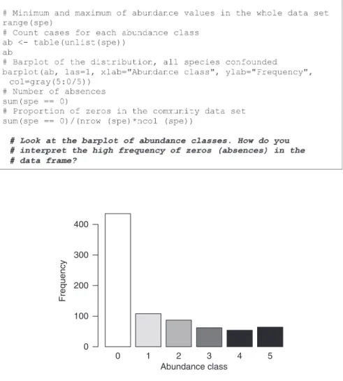
spe created above). Verneaux used a semi-quantitative, species-specific, abun-dance scale (0–5) so that comparisons between species abunabun-dances make sense. However, species-specific codes cannot be understood as unbiased estimates of the true abundances (number or density of individuals) or biomasses at the sites.
Fig. 2.1 Barplot of abundance classes 0 1 2 3 4 5 Abundance class Frequency 0 100 200 300 400
2.2.3 Species Data: A Closer Look
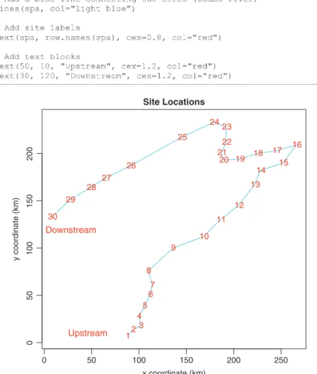
The commands above give an idea about the data structure. But codes and numbers are not very attractive or inspiring, so let us illustrate some features. We first create a map of the sites (Fig. 2.2):
Fig. 2.2 Map of the 30 sampling sites along the Doubs River
0 50 100 150 200 250 0 50 100 150 200 Site Locations x coordinate (km) y coordinate (km) 12 3 4 5 67 8 9 10 11 12 13 14 15 16 17 18 19 20 21 22 23 24 25 26 27 28 29 30 Upstream Downstream
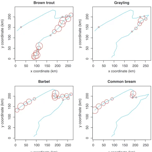
Now, the river looks more real, but where are the fish? To show the distribution and abundance of the four species used to characterize ecological zones in European rivers (Fig. 2.3), one can type:
Hint Note the use of the cex argument in the plot() function: cex is used to define the size of an item in a graph. Here its value is a vector of the spe data frame, i.e. the abundances of a given species (e.g.
cex=spe$TRU). The result is a series of bubbles whose diameter at each site is proportional to the species abundance. Also, since the object spa contains only two variables x and y, the formula has been simplified by replacing the two first arguments for horizontal and ver-tical axes by the name of the data frame.
At how many sites does each species occur? Calculate the relative frequencies of species (proportion of the number of sites) and plot histograms (Fig. 2.4): Fig. 2.3 Bubble maps of the abundance of four fish species
0 50 100 150 200 250 0 50 100 150 200 Brown trout x coordinate (km) y coordinate (km) 0 50 100 150 200 250 0 50 100 150 200 Grayling x coordinate (km) y coordinate (km) 0 50 100 150 200 250 0 50 100 150 200 Barbel x coordinate (km) y coordinate (km) 0 50 100 150 200 250 0 50 100 150 200 Common bream x coordinate (km) y coordinate (km)
Hint Examine the use of the apply() function, applied here to the columns of the data frame spe. Note that the first part of the function call (spe > 0) evaluates the values in the data frame to TRUE/ FALSE, and the number of TRUE cases per column is counted by summing.
Fig. 2.4 Frequency histograms: species occurrences and relative frequencies in the 30 sites
Species Occurrences Number of occurrences Number of species 0 5 10 15 20 25 30 0 2 4 6 8 10 12
Species Relative Frequencies
Frequency of occurrences (%) Number of species 0 20 40 60 80 100 0 1 2 3 4 5 6 7
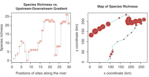
Now that we have seen at how many sites each species is present, we may want to know how many species are present at each site (species richness, Fig. 2.5):
Hint Observe the use of the type="s" argument of the plot() function to draw steps between values.
Hint Note the special use of function rowSums() for the computation of species richness N0. Normally, rowSums(array) computes the sums of the rows in that array. Here, argument spe > 0 calls for the sum of the cases where the value is greater than 0.
Finally, one can easily compute classical diversity indices from the data. Let us do it with the function diversity() of the vegan package.
Fig. 2.5 Species richness along the river
0 5 10 15 20 25 30 0 5 10 15 20 25 Species Richness vs. Upstream-Downstream Gradient
Positions of sites along the river
Species richness 1 23 4 5 6 7 8 910111213 1415 16 171819202122 23 2425 262728 29 30 0 50 100 150 200 250 0 50 100 150 200
Map of Species Richness
x coordinate (km)
Hill’s numbers (N), which are all expressed in the same units, and ratios (E) derived from these numbers, can be used to compute diversity indices instead of popular formulae for Shannon entropy (H) and Pielou evenness (J). Note that there are other ways of estimating diversity while taking into account unobserved species (e.g. Chao and Shen 2003).
2.2.4 Species Data Transformation
There are instances where one needs to transform the data prior to analysis. The main reasons are given below with examples of transformations:
Make descriptors that have been measured in different units comparable (ranging, •
standardization to z-scores, i.e. centring and reduction, also called scaling) Make the variables normal and stabilize their variances (e.g. square root, fourth •
root, log transformations)
Make the relationships among variables linear (e.g. log transformation of •
response variable if the relationship is exponential)
Modify the weights of the variables or objects (e.g. give the same length •
(or norm) to all object vectors)
Code categorical variables into dummy binary variables or Helmert contrasts •
Species abundances are dimensionally homogenous (expressed in the same physical units), quantitative (count, density, cover, biovolume, biomass, frequency, etc.) or semi-quantitative (classes) variables and restricted to positive or null values (zero meaning absence). For these, simple transformations may be used to reduce the importance of observations with very high values: sqrt() (square root),
sqrt(sqrt()) (fourth root), or log1p() (natural logarithm of abundance + 1 to keep absence as zero) are commonly applied R functions. In extreme cases, to give the same weight to all positive abundances irrespective of their values, the data can be transformed to binary 1-0 form (presence–absence).
The decostand() function of the vegan package provides many options for common standardization of ecological data. In this function, standardization, as contrasted with simple transformation (such as square root, log or presence–absence), means that the values are not transformed individually but relative to other values in the data table. Standardization can be done relative to sites (site profiles), species (species profiles), or both (double profiles), depend-ing on the focus of the analysis. Here are some examples illustrated by boxplots (Fig. 2.6):
Hint Take a look at the line: norm <- function(x) sqrt(x%*%x). It is an example of a small function built on the fly to fill a gap in the stan-dard R packages: this function computes the norm (length) of a vector
using a matrix algebraic form of Pythagora’s theorem. For more matrix algebra, visit the Code It Yourself corners.
Another way to compare the effects of transformations on species profiles is to plot them along the river course:
Fig. 2.6 Boxplots of transformed abundances of a common species, Nemacheilus barbatulus (stone loach)
raw data sqrt log 0 1 2 3 4 5 Simple transformation max total 0.0 0.2 0.4 0.6 0.8 1.0 Standardization by species
Hellinger total norm 0.0 0.1 0.2 0.3 0.4 0.5 0.6 Standardization by sites Chi-square Wisconsin 0.0 0.2 0.4 0.6 0.8 1.0 1.2 Double standardization
The Code It Yourself corner #1
Write a function to compute the Shannon–Weaver entropy for a site vector containing species abundances. The formula is:
[
i log( )i]
H′ = −
∑
p × pwhere pi = ni / N and ni = abundance of species i and N = total abundance of all species.
After that, display the code ofvegan’sfunctiondiversity()to see how it has been coded among other indices by Jari Oksanen and Bob O’Hara. Nice and compact, isn’t it?
2.2.5 Environmental Data
Now that we are acquainted with the species data, let us turn to the environmental data (object env).
First, go back to Sect. 2.2.2 and apply the basic functions presented there to
env. While examining the summary(), note how the variables differ from the species data in values and spatial distributions.
Draw maps of some of the environmental variables, first in the form of bubble maps (Fig. 2.7):
Hint See how the cex argument is used to make the size of the bubbles comparable among plots. Play with these values to see the changes in the graphical output.
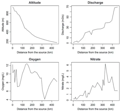
Now, examine the variation of some descriptors along the stream (Fig. 2.8): Fig. 2.7 Bubble maps of environmental variables
0 50 100 150 200 250 0 50 100 150 200 Altitude x y 0 50 100 150 200 250 0 50 100 150 200 Discharge x y 0 50 100 150 200 250 0 50 100 15 0 200 Oxygen x y 0 50 100 150 200 250 0 50 100 150 200 Nitrate x y
Fig. 2.8 Line plots of environmental variables
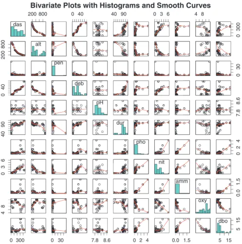
To explore graphically the bivariate relationships among the environmental variables, we can use the powerful pairs() graphical function, which draws a matrix of scatter plots (Fig. 2.9).
Hint Each scatterplot shows the relationship between two variables identi-fied on the diagonal. The abscissa of the scatterplot is the variable above or under it, and the ordinate is the variable to its left or right.
Moreover, we can add a LOWESS smoother to each bivariate plot and draw histograms in the diagonal plots, showing the frequency distribution of each vari-able, using external functions of the panelutils.R script.
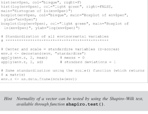
Simple transformations, such as the log transformation, can be used to improve the distributions of some variables (make it closer to the normal distribution). Furthermore, because environmental variables are dimensionally heterogeneous (expressed in different units and scales), many statistical analyses require their standardization to zero mean and unit variance. These centred and scaled variables are called z-scores. We can now illustrate transformations and standardization with our example data (Fig. 2.10).
Fig. 2.9 Scatter plots between all pairs of environmental variables with LOWESS smoothers das 200 800 0 40 40 90 0 3 6 4 8 0 300 200 800 alt pen 0 30 0 40 deb pH 7.8 8.6 40 90 dur pho 0 2 4 0 3 6 nit amm 0.0 1.5 4 8 oxy 0 300 0 30 7.8 8.6 0 2 4 0.0 1.5 5 15 5 15 dbo
Hint Normality of a vector can be tested by using the Shapiro–Wilk test, available through function shapiro.test().
Fig. 2.10 Histograms and boxplots of the untransformed (left) and log-transformed pen variable (slope) Histogram of env$pen env$pen Frequency 0 10 20 30 40 50 0 5 10 20 30 Histogram of ln(env$pen) log(env$pen) Frequency −2 −1 0 1 2 3 4 0 2 4 6 8 10 0 10 20 30 40 Boxplot of env$pen env$pen − 1 0 1 2 3 4 Boxplot of ln(env$pen) log(env$pen )
2.3 Conclusion
The tools presented in this chapter allow researchers to obtain a general impression of their data. Although you see much more elaborate analyses in the next chapters, keep in mind that a first exploratory look at the data can tell much about them. Information about simple parameters and distributions of variables is important to consider in order to choose more advanced analyses correctly. Graphical represen-tations like bubble maps are useful to reveal how the variables are spatially orga-nized; they may help generate hypotheses about the processes acting behind the scene. Boxplots and simple statistics may be necessary to reveal unusual or aberrant values.
EDA is often neglected by people who are eager to jump to more sophisticated analyses. We hope to have convinced you that it should have an important place in the toolbox of ecologists.