Structure
evolution
in
electrorheological
fluids
flowing
through microchannels
Bian Qian, Gareth H. McKinley, and Anette Hosoi
∗Received Xth XXXXXXXXXX 20XX, Accepted Xth XXXXXXXXX 20XX First published on the web Xth XXXXXXXXXX 20XX
DOI: 10.1039/b000000x
Enhanced knowledge of the transient behavior and characteristics of electrorheological (ER) fluids subject to time dependent electric fields carries the potential to advance the design of fast actuated hydraulic devices. In this study, the dynamic response of electrorheological fluid flows in rectilinear microchannels was investigated experimentally. Using high-speed microscopic imaging, the evolution of particle aggregates in ER fluids subjected to temporally stepwise electric fields was visualized. Nonuniform growth of the particle structures in the channel was observed and correlated to field strength and flow rate. Two competing time scales for structure growth were identified. Guided by experimental observations, we develop a phenomenological model to quantitatively describe and predict the evolution of microscale structures and the concomitant induced pressure gradient.
Introduction
Electrorheological (ER) fluids are materials whose rheo-logical characteristics can be altered through the applica-tion of an external electric field1. Typical ER fluids
con-sist of micron-sized non-conductive or weakly-conductive particles suspended in an insulating fluid. Upon the ap-plication of a strong electric field, the particles become polarized and aggregate via electrostatic interactions, into columns aligned along the field direction. The forma-tion of columnar structures induces a dramatic increase in the apparent fluid viscosity, leading to a phase transition in ER fluids from a liquid to a solid-like state. Such tran-sitions occur rapidly and are generally reversible when the electric field is removed. These unique features make ER fluids an ideal class of materials for use in a variety of hydraulic components, including valves2,3, clutches4 and
shock absorbers5. Recently, custom-formulated ER fluids
have been employed in a number of microscale applica-tions6–8 and in various microfluidic devices9–12. With
the recent discovery of nanoparticle-based ER fluids13,
the expansion of applications to even smaller scale de-vices can also be envisioned. As a result of this versa-tility, ER fluids have been of continuing interest to the scientific and engineering communities since their discov-ery. Over the past few decades, numerous research efforts have been made to enhance our fundamental understand-ing of these materials and a prominent theme that arises in these studies centers on the question of the dynamic ER material response.
Early rheology measurements show that the stress
re-sponse of an ER fluid subject to a temporally stepwise electric field is not only dependent on fluid chemistry but also on flow conditions14. For ER fluids undergoing steady shear, the characteristic time for the shear stress to reach steady state is proportional to shear rate and only weakly dependent on electric field strength. The shear-rate dependence of the stress response was con-firmed in later experiments and an exponential increase in shear stress over time was observed15,16. This
shear-rate dependence of the stress response was ascribed to a hypothesized rate-dependence associated with column breakup and formation. However, this explanation lacked supporting evidence owing to the technical challenges as-sociated with direct observation of the evolution of par-ticle structures.
Further investigations of the shear response of ER flu-ids have revealed that the increasing shear stress passes through three sequential stages17. In the first stage, the
shear stress climbs dramatically; this stage occurs on the scale of several tens of milliseconds. During the second stage, the stress increases more moderately. In the last stage, the increase of shear stress is slow and the growth persists for several seconds. A similar temporal response was observed in the optical response of ER fluids18–20; the
measured light transmittance of a quiescent ER suspen-sion displayed a significant transmittance enhancement upon the application of electric field. Following the ini-tial enhancement, the transmitted light intensity continu-ously increased but at a reduced rate, eventually reaching a plateau. Since the variation of light transmittance is a direct result of changes in the microstructure, the
corre-spondence between the stress and optical response of ER fluids suggests a correlation between the stress increase and structure evolution. However, in the absence of di-rect observation of structure growth under relevant flow conditions, the details of this relationship remain unclear. Thanks to advances in high speed imaging, real-time visualization of structure formation in ER fluids has re-cently become feasible. The first such experiments were carried out to observe structure formation in a quiescent ER fluid and measurements correlating particle concen-tration and field strength were performed21,22. A clear dependence of structure formation time on particle con-centration and field strength was found. Further investi-gations revealed that the structure growth – like the evo-lution of stress – is comprised of three stages23,24. In the
earliest stage, randomly distributed particles become po-larized and aggregate into chains. Subsequently, individ-ual chains coalesce into metastable columns. In the final stage, these metastable columns grow into thicker stable columnar structures. These three stages correspond to the three previously observed periods of stress response and the duration of each stage of structure growth was found to be comparable to the corresponding stages ob-served in stress measurements. In addition to these ex-perimental observations, a number of simulation studies have been carried out to advance understanding of the rheology and kinetics of structure formation in ER flu-ids25–29.
These previous studies, however, concentrated on ER fluids in steady shear (Couette flow) or in a quiescent state. For ER fluids in a pressure-driven flow mode (Poiseuille flow), only a few publications exist, despite the relevance of this flow type in many electrorheological applications such as flow valves and dampers. In contrast to direct measurements of the wall shear stress, pressure drop – which quantifies the driving force required to push fluid through a channel of a prescribed geometry at a given flow rate – is typically measured to characterize the response of ER fluids in flow mode. Previous experiments have shown that the evolution in the pressure drop of ER flows in a channel is a nonlinear function of the time that the electric field has been applied30. The transient time
to achieve a steady pressure drop was found to depend on field strength, temperature and particle conductivity. To rationalize this transient pressure drop, a Bingham-fluid-based model was recently proposed31,32. Computed
pressure responses from the proposed model are in good agreements with the experimental measurements, how-ever, the parameters employed in the model cannot be independently determined without additional knowledge of their physical origins.
Further experimental investigations to observe
struc-ture growth in ER fluids33,34have found that the rate of
structure growth and the maximum size of the individual structures are determined by the competition between the field-induced particle interaction force and hydrody-namic forces. Similar dependencies were also observed in flowing magnetorheological fluids35. Corresponding
pressure measurements indicate that the pressure drop is strongly dependent on field strength, which is in con-sistent with the results obtained for ER fluids in shear geometries. The field-strength dependence of the pres-sure response can be rationalized qualitatively from the observed structure growth. However, a quantitative cor-relation between pressure drop and structure growth has not yet been achieved in these studies. In addition, al-though spatial variation in the microstructure was briefly mentioned in previous studies33,34, a systematic
investi-gation of these variations and the resultant effect on the net pressure drop has not been performed.
In the present study, we experimentally investigate the evolution of microstructure in ER fluids under a range of shear rates, between 90 s−1 and 400 s−1. Our study is focused to fluids flowing in rectilinear microchannels and undergoing a temporally stepwise electric field. We aim at understanding the aggregate structure growth across the entire channel and its dependence on flow conditions, rather than the formation of a single column. In addi-tion, the transient pressure drop across the channel is correlated to the structure growth by evaluating the re-sistance ∆QP from the structure to the fluid flow, a ratio of the pressure drop ∆P to the flow rateQ. We present the pressure data in the form of flow resistant ∆P
Q because
∆P
Q can be used conveniently by people in designing chan-nels for valves and dampers (i.e. what ∆P is required for a given Q). Finally, we construct a phenomenological model to complement the experimental observations.
Experimental Methods
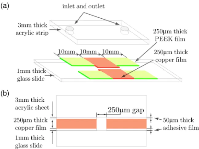
A transparent rectangular microchannel was designed and fabricated for our study. Figure 1 shows the config-uration of the channel, which consists of three sections: a test section for flow visualization, and two auxiliary sections at the entry and the exit. In the test section, two pieces of 250µm thick and 10 mm long copper film were used to form the channel walls, separated by a uni-form 250µm gap. In the auxiliary sections, the channel walls are made up of non-conductive polyether ether ke-tone film (250µm thick, 10 mm long) with a separation
Hatsopoulos Microfluids Laboratory, Department of Mechani-cal Engineering, Massachusetts Institute of Technology, 77 Mas-sachusetts Avenue, Cambridge, MasMas-sachusetts 02139. Fax: +1 617-253-8559; Tel: +1 617-253-4337; E-mail: [email protected]
1mmthick glassslide 250µmthick copperfilm 3mmthick acrylicstrip inletandoutlet 250µmthick PEEKfilm 10mm 10mm 10mm 250µmgap 250µmthick copperfilm 3mmthick acrylicsheet 1mmthick glassslide 50µmthick adhesivefilm (a) (b)
Fig. 1 (a) Schematic of a microchannel fabricated for flow visualization and pressure measurements. (b) Cross-sectional view of the microchannel in the flow direction.
of 3 mm. To form a closed channel, these films were ad-hered, using a 50µm thick adhesive film (3M, 966), to a 1 mm thick glass slide and a 3 mm thick acrylic strip serv-ing as a cover sheet. At either end of the flow channel, tapped holes were fabricated in the cover sheet to mount the inlet and the outlet adapter. To apply the electric field within the flow channel, the conductive copper chan-nel walls were connected to a high voltage power supply (Stanford Research PS350) via a driver circuit board. Us-ing external triggers, the electric field can be switched on and off via the driver circuit board and synchronized with measurement devices.
For flow imaging, the microfluidic chip was mounted onto an inverted optical microscope (Nikon TE-2000S). The flow channel was illuminated from above by a col-limated light source and viewed with a 2X microscope objective (NA=0.06) from below. A high speed camera (Phantom V5) connected to the microscope was used to record the structure evolution at a frame rate of 400 fps. With these optical arrangements, the depth of field of the imaging system was 240µm and the image resolution 8.5µm/pixel.
The ER fluid used in the experiments was a colloidal suspension of polyurethane particles with silicone oil as a carrier fluid (Fluidicon, RheOil4). The mean diameter of the dielectric particles is 2µm and its volume fraction in the stock solution isφf,in= 0.41. For imaging purposes,
the stock solution was diluted with 100 cSt silicone oil to φf,in = 0.02 in all experiments. The prepared
parti-cle solution was injected into the flow channel using a gas-tight glass syringe (Hamilton, 1005TLL) which was connected to the flow channel via stainless steel tubes. To maintain a continuous fluid flow within the channel, a
sy-ringe pump (Harvard Apparatus, PHD Ultra) was used to control the flow rate Q in a range of 20-80µL/min. The shear rate at this flow rate is estimated to be 95-380 s−1 from reference36. A differential pressure sensor (Honeywell, 26PCBFA6D) with a measurement range of 34.47 kPa was inserted to measure the pressure drop be-tween the entry and the exit of the flow channel. Signals from the pressure sensor were amplified and acquired by a data acquisition card (National Instrument, DAQ1200).
Experimental Results and Discussion
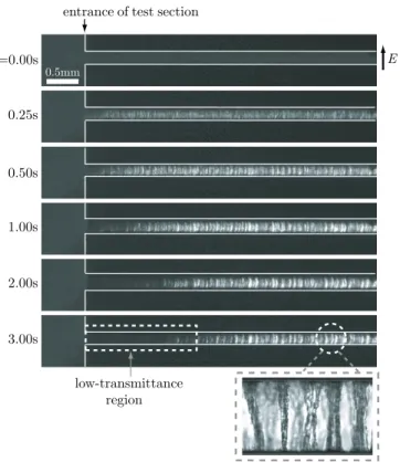
Typical images of the structure evolution in the ER flow within a microchannel are shown in Figure 2. In the ab-sence of an applied electric field, particles disperse uni-formly throughout the carrier fluid. Owing to the differ-ence of refractive index between particles and base fluid, the illuminating light is scattered multiple times as it propagates through the particle solution, resulting in a low transmittance of light. Therefore, the image of the flow in the channel appears as a uniform gray ribbon as shown in Figure 2 (top row). By contrast, when an elec-tric field is applied, particles rapidly aggregate into small clusters and columns. As a result of this phase separa-tion, voids and columns are formed, alternating along the channel and resulting in a spatial variation in transmit-tance of light. At locations of large voids, light is trans-mitted with little loss and the corresponding regions are bright in the image. In regions where particles are closely packed, most of the illumination light is blocked, result-ing in dark shadowed regions. Regularly spaced columnar structures appear as stripes as shown in the lowermost panel of Figure 2.
Following the initial structure formation, the columns initially formed coarsen and new columns form as fresh particle-laden fluid flows into the channel. Continuous coarsening and densification leads to a reduction of poros-ity and a concomitant decrease in optical transmission across the channel. As the number of columns and the thickness of each individual column increase, the parti-cle density reaches a critical value above which almost all of the illumination light is blocked, leaving a con-tinuous dark region as highlighted in Figure 2. This low-transmittance region first appears near the entry and then expands continuously downstream, indicating a faster structure growth rate in the upstream regions. We attribute this inhomogeneous structure growth to the uneven spatial distribution of flowing particles inside the channel. At the entrance, fresh particles are continu-ously injected and therefore the volume fractionφfof free
(i.e. unstuck) particles is high. As particles flow down the channel, some of them adhere to existing fixed columnar
t=0.00s 0.25s 0.50s 1.00s 2.00s 3.00s 0.5mm entranceoftestsection low-transmittance region E
Fig. 2 Images of structure formation and subsequent coars-ening during pressure-driven flow of an ER suspension inside a straight microchannel. The channel is 250µm wide (between the upper and lower electrodes) and 350µm deep (into the page). The channel walls are indicated with white lines. The particle suspension (2% v/v) flowed from left to right at a con-stant flow rate of 60µL/min. An electric field E=4kV/mm was applied perpendicular to the channel walls att= 0. A low-transmittance region which is densely packed with parti-cle columns is highlighted in the final image at the bottom left. The figure insert at the bottom right is a close-up of the loosely spaced particle columns.
structures, resulting in a reduction of number of available free particles downstream. Assuming the rate at which free particles become stuck particles is linearly propor-tional to the number of available free particles, it follows that the number of flowing particles decreases exponen-tially with distancexdown the channel. Therefore, close to the entrance structures grow more rapidly.
However, the local volume fraction of stuck particles
φs(x) cannot grow indefinitely since a minimum porosity
must be maintained to allow for continuous fluid flow; as
φsincreases, the resistance to fluid flow increases. As a
re-sult, the hydrodynamic stressτhon the particle columns
increases untilφsreaches a critical value, at which the
hy-drodynamic stresses exert the maximum stressτythat the
column can withstand. Above this critical value, the col-umn breaks, causing a local reduction ofφswhich leads to
a new round of column formation. These processes of col-umn breakup and formation result in an average steady state value for φs at which the local volume fraction of
stuck particle achieves a maximum, φs,max. In regions
whereφs(x) =φs,max, no net additional flowing particles
are trapped. Instead they move with the fluid flow to-ward regions ofφs(x)< φs,max, driving the expansion of
the low-transmittance region.
The competition of τy and τh determines the
maxi-mum volume fractionφs,max of stuck particle. The
Ma-son number37,38, which is defined by Mn = τy
τh, is used
to characterize the relative importance of τy to τh. We
expect the hydrodynamic stress to scale asτh∼f(φs)ηQAL
where f(φs) is an increasing function ofφs, Aand Lare
the cross sectional area and the length of flow channel, respectively. In addition, the yield stress τy(E) is
ex-pected to increase with field strength E. Sinceφs,max is
achieved when Mn ∼ 1, φs,max ∼ f−1(ALη τyQ(E)). From
this scaling, we expectφs,maxto increase with increasing
E and decrease with increasingQ.
To quantify how the field strength E and flow rate
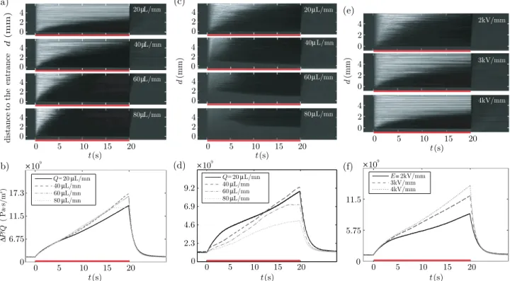
Qaffect structure growth, experiments were carried out over a range of flow rates and electric fields. To simplify comparison among different tests, a two dimensional in-tensity map was generated to display the evolution of particle structures, as illustrated in Figure 3(a). The in-tensity map is an aggregate of the channel center lines shown in Figure 2. Each vertical line on the aggregate map is a snapshot in time. The gray value on the map measures the intensity of the transmitted light and thus it is an indication of the local particle concentration. As the maps show, at the beginning of the image acquisition, no electric field is applied to the channel and the trans-mitted light intensity is constant along the vertical line (corresponding to the dark region fort <0 in Figure 3). However, when the electric field is applied att= 0,
parti-0 2 4 0 2 4 0 2 4 0 5 10 15 20 0 2 4 t(s) distance to the ent rance d ( mm ) (a) 0 6.75 11.5 17.3 t(s) Q=20µL/mn 40µL/mn 60µL/mn 80µL/mn (b) 0 2 4 0 2 4 0 2 4 0 5 10 15 20 0 2 4 d ( mm ) t(s) (c) 20µL/mn 40µL/mn 60µL/mn 80µL/mn 0 2.3 4.6 6.9 9.2 t(s) Q=20µL/mn 40µL/mn 60µL/mn 80µL/mn (d) 0 2 4 0 2 4 0 5 10 15 20 0 2 4 t(s) d ( mm ) (e) 2kV/mm 3kV/mm 4kV/mm 0 5.75 11.5 t(s) E=2kV/mm 3kV/mm 4kV/mm (f) 0 5 10 15 20 0 5 10 15 20 0 5 10 15 20 ∆ P / Q ( P a s /m ) 3 9 . 10 109 109 20µL/mn 40µL/mn 60µL/mn 80µL/mn
Fig. 3(a) Intensity maps displaying structure evolution in a microchannel with an applied electric field ofE=4 kV/mm. Each vertical line on the map is an extraction of the image pixels along the center line of the flow channel from the experimental images as shown in figure 2. The map represents the temporal evolution of transmitted light and the temporal change of number of particles aggregates along the channel. Maps are shown for four different flow rates, 20, 40, 60 and 80µL/min. The red line on each plot indicates the states of electric field (red = on). (c) Intensity maps for flows with a relatively low electric field E = 2 kV/mm. (e) Intensity maps at a constant flow rate, Q = 20µL/min, with varying electric field strengths. (b)(d)(f) Measurements of flow resistance ∆P
cles begin to aggregate and columns form. Fixed particle columns appear as a thin horizontal gray lines on the intensity maps. Subsequent to the initial column forma-tion, more and more particles accumulate at the entry, indicated by a growing region of high particle concentra-tion and low transmittance. On the intensity map, the lower black segment of each vertical line corresponds to an instantaneous image of the growing low-transmittance particle-rich region. The edge of the dark region on the intensity map represents the front of the growing low-transmittance region. After the electric field is switched off, the particle columns are progressively washed out and the channel refills with evenly dispersed moving particles with volume fractionφf = 0.02 (as indicated by the
uni-form dark gray area at late times).
Using the generated intensity maps, we first compare the structure growth at different flow rates with a fixed electric field strength E=4 kV/mm. As shown in fig-ure 3(a), all intensity maps show similar featfig-ures when the electric field is applied. At the initial stage, loosely spaced columns build up along the entire channel. Subse-quently a low-transmittance region forms around the en-try and grows along the flow direction. However, the rate of growth of the low-transmittance region is observed to vary with the fluid flow rate Q: the higher the flow rate the faster the low-transmittance region expands. The change in expansion rate is partly attributed to the vari-ation in the rate at which particles are delivered at the inlet. At high flow rates more particles flow into the channel per unit time, increasing the rate of particle de-livery and accelerating the structure growth. If φs,max
is independent of flow rate, it follows that the flow re-sistance ∆QP builds up more rapidly with increasing flow rate. Measurements of ∆P
Q (figure 3(b)) indeed show a more rapid increase in∆QP whenQis increased from 20 to 40µL/min. However, further increase of flow rate from 40µL/min to 60µL/min and to 80µL/min does not pro-mote additional change in flow resistance, suggesting that
φs,maxis itself a function of flow rateQ. As discussed
pre-viously,φs,maxis expected to decrease with increasingQ.
Therefore, ∆QP might not grow with further increase inQ
since ∆QP is not only determined by the total number of particles flowing into the channel but also by the spatial distribution of particles.
Following measurements at high electric fields, we per-formed a series of experiments at relatively low fields in which the flows exhibit markedly different behavior. As shown in figure 3(c), no stripes are present on the in-tensity maps except at the lowest flow rate, indicating that no fixed particle columns built up along the chan-nel. Although particles still aggregate into small clusters
when the electric field is applied and the flow resistance increases, the interactions between these particle clusters and the channel walls are not strong enough to resist hy-drodynamic stresses and form stationary columns span-ning the channel. Instead the particle clusters move with the fluid flow, leading to random temporal variations in local light transmittance. Although no fixed structures form, particle aggregation still enhances light transmit-tance, resulting in a lighter average gray intensity. This transmittance enhancement becomes weaker as flow rate increases, indicating a slow and relatively weak cluster-ing process at high flow rates. At late stages, even at these low fields and high flow rates, some particle clus-ters may grow sufficiently large, occasionally leading to a fixed particle column that forms across the channel. Once this column nucleates, more and more particle columns form. Correspondingly, on the intensity map, a dark spot emerges at some distance away from the entry and grows both toward the entrance and the exit. The formation of the first fixed column appears to be random and the subsequent growth of the particle dense region is difficult to predict quantitatively. However, a general trend is ob-served for the first appearance of the fixed column: as flow rate increases, the fixed column appears at a loca-tion further away from the entry and at later times. This observation suggests that the higher the flow rate, the smaller the probability of building a full-length column that spans the channel.
Corresponding flow resistance measurements across the channel reveal that the first formation of fixed particle chains is critical to the initial growth of flow resistance. As shown in figure 3(d), the flow resistance builds up fastest at the lowest flow rate. As flow rate increases, flow resistance grows more slowly until fixed chains start building in the channel. This retarded growth of flow resistance with increasing flow rate is in contrast to the enhanced growth in flow resistance at high electric fields. Comparisons were also performed for flows under dif-ferent electric fields as shown in figure 3(e). At a low flow rate Q=20µL/min, fixed columns build along the entire channel upon application of the electric field. Fol-lowing this initial formation, column coarsening and den-sification progresses. As before, a particle dense region forms near the entry and expanded. It is seen from the maps that under a lower electric field the front of the low-transmittance region propagates at a higher speed. This observation indicates a higher φs,max in the
low-transmittance region as field strength increases since the rate at which particles flow into the channel is the same for all three tests. Note that although a stronger elec-tric field leads to faster particle aggregation, the speed of structure growth is less dependent on the strength of
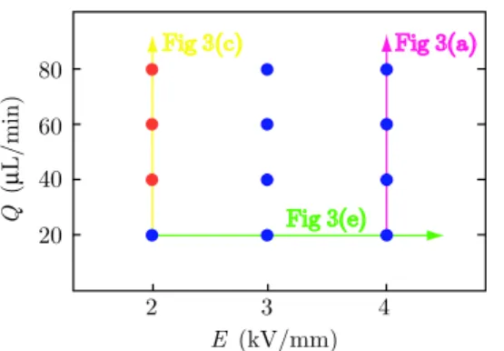
2 3 4 20 40 60 80 E (kV/mm) Q ( µ L /m i n )
Fig. 4A schematic diagram illustrating the different regimes of structure growth. Dots represent experimental tests at dif-ferent settings of Q andE. Colors are used to indicate the types of structure growth: limited by column stability (red) and limited by particle delivery (blue). Typical intensity maps are shown in Fig. 3 for displaying structure growth.
electric field, and rather is limited primarily by the rate of particle delivery.
In accordance with the measured structure growth, the flow resistance built up rapidly under all tested electric fields. At early stages, the growth of flow resistance is al-most indistinguishable between different fields. However, at late stages, a faster growth rate is observed in ∆P
Q un-der higher electric fields. This observation reveals that the flow resistance is not only determined by the total number of particles stuck in the channel but also deter-mined by the spatial distribution of the stuck particles.
Two modes of structure growth are thus identified: lim-ited by chain stability and limlim-ited by particle delivery. For the first one, the hydrodynamic stress is initially high and particle interaction is week. Therefore, parti-cle chains easily break under hydrodynamic stress and stationary chains seldom form across the channel. Mi-crochannel flows operating at highQunder lowEfall into this category. For the second one, hydrodynamic stress is initially low compared to the inter-particle stress. When the electric field is applied, columns spanning over the gap between electrodes form immediately. As free parti-cles are recruited from the incoming flow, columns grow continuously. Since the time for initial column formation is short, the speed of structure growth is limited by parti-cle delivery. Such a mode of structure growth is observed in flows operating at lowQwith highE. A schematic di-agram shown in figure 4 illustrates the different regimes of structure growth.
In addition to qualitative descriptions, we quan-titatively measure the expansion rate of the low-transmittance region by extracting the front position from the intensity map. The front evolution curves
pre-0 2 4 0 2 4 0 2 4 0 5 10 15 20 0 2 4 t(s) d ( mm ) (a) 20 µL/mn 40µL/mn 60µL/mn 80µL/mn 0 5 10 15 20 0 1 2 3 4 5 t(s) d ( mm ) 20µL/mn 40µL/mn 60µL/mn 80µL/mn (b) 0 0.2 0.4 0.6 0 1 2 3 4 5 t/tc (c) d ( mm )
Fig. 5 Expansion of low-transmittance regions at different flow rates. (a) Extracted moving fronts (yellow lines) of the low-transmittance regions plotted on top of the respective the intensity maps. (b) Front movements obtained in (a) for dif-ferent flow rates. (c) Scaled front movements.
sented in figure 5(a) are obtained by first converting the intensity map to a binary image using thresholding and then tracing the boundary of the largest connected clus-ter on the converted binary map. The threshold value for image conversion is selected to be the mean gray in-tensity of the flow image under E = 0 kV/mm. The extracted front locations for different Q are plotted in figure 5(b). All front evolution curves display a quasi-linear increase at short times. The slope of the curve increases with flow rate. Since the slope measures the expansion speed of the low-transmittance region, it can be expressed as Qφf,in
A(φs,max−φf,in)
in whichQis the fluid flow rate,Athe cross-sectional area of the flow channel,φf,in
the volume fraction of free particles in the fluid in the absence of electric fields and φs,max the maximum
vol-ume fraction of stuck particles in the channel. With the average measured slopes and the prescribed experimen-tal parametersQ, φf,in and A, φs,max= 0.45, 0.36, 0.31
and 0.27 can be obtained for corresponding flow rates
Q=20, 40, 60 and 80µL/min, respectively. The decrease ofφs,max with increasingQis in agreement with our
ini-tial expectation. Using the estimatedφs,max, we define a
characteristic timetc= AL(φs,max−φf,in) Qφf,in
which character-izes the time scale to fill the channel with particles that are delivered by the incoming fluid stream. By normaliz-ing timet with the defined tc, all front evolution curves
collapse on to a single curve as shown in figure 5(c).
Model
The experimental observations described above are markedly different from anything that could be simulated
with a continuum model, e.g. Bingham flow in a chan-nel31,34,39,40. The Bingham fluid model is commonly used
to describe the macroscopic plastic behaviors of ER sus-pensions and it is useful for predicting the steady pressure drop of ER flows in a channel. However, the Bingham fluid model is not itself amenable to description via a mi-croscopic view of suspension structure. Therefore, it does not allow one to capture any structure evolution along the channel and hence precisely predict the transient pressure drop across the channel.
Guided by the experimental observations, we construct a simple model for describing the evolution of particle structures and the accompanied change of flow resistance. Since the size of a particle and the radius of a particle column are both small compared to the length of the flow channel, we take a continuum approach to model particle distribution. With this assumption, the volume fraction of stuck particlesφs(x, t) and the volume fraction of free
particles φf(x, t) can be approximated as a continuous
function of timetand distance from the entrancex. Note thatφsis computed relative to the volume of channel slice
Adx while φf is defined relative to the volume of fluid
within this slice, A(1−φs)dx. With these definitions of
φf andφs, conservation of particles can be expressed as
∂φf(1−φs) ∂t +u(1−φs) ∂φf ∂x + dφs dt = 0, (1)
in whichu(x, t) is the average local flow speed. For a con-stant flow rate,ucan be related toφsbyu=A(1Q−φs). 1D
plug flow is assumed in the model so that uis constant across the cross section perpendicular to the channel axis. The first term in equation 1 represents the rate of change of the number of free particles. The second term describes the change of free particles due to flow convection. The final term denotes the rate of change from free particles into stuck particles. To get a closed-form solution for equation 1, an expression for dφs
dt is required. Since the particle dense region exhibits a quasi-linear expansion at short times, we assume that the growth of stuck particles
dφs
dt is linearly proportional to the number of free parti-cles in the fluid phase,αφf(1−φs). The proportionality
constant α represents the probability for a free particle become incorporated into the structure per unit time and it is a measurement of the time scale for particle aggrega-tionα−1. For simplicity,αis assumed to be constant for fixedE. Given this, an equation for the volume fraction growth of stuck particles can be written as
dφs
dt =α(E)φf(1−φs){1−erf[ Q
M A− P(E)]}, (2)
in which the growth ofφsis cutoff with an error function.
The argument of the error function M AQ −P(E) is a com-parison between the hydrodynamic stress on the particle
structures and the holding stress of particle columns. The maximum pressure gradient which the particle structures can sustain is given byP. SinceP measures the strength of particle-particle attraction, it is primarily determined by the strength of the applied electric field E. Growth in the number of stuck particles is arrested when this maximum pressure gradient is comparable to the local pressure drop M(x,tQ)AwhereM(x, t) is the flow mobility. Flow mobility is a monotonically decreasing function of
φs. The error function defines a maximum fraction of
stuck particlesφs,max above which M AQ − P(E) becomes
positive and the growth ofφsstops.
To relate the local flow mobilityM(x, t) toφs(x, t), the
particle columns are assumed to be an array of cylinders in a hexagonal packing arrangement. With this approx-imation, the flow mobility can be calculated using the analytical expression obtained in41,
M = M1ξ1+M2ξ2, (3) in which M1 = 1 3√3 r2 η (1−l2)2 l " 3arctanp (1 +l)/(1−l) √ 1−l2 +l 2 2 + 1 −1 , (4) and M2= r2l2 4η ( 1 8l− 4−s s2 )− 1. (5) Here l = 2√3 π φs, s = lnl− 3 4 +l 2−1 4l− 4, η is the fluid
viscosity andris the radius of the particle column. The mobility coefficients M1 and M2 represent the flow
mo-bility obtained for high and low φs, respectively. They
are only valid for φs at the extreme ends. To calculate
M over a wide range ofφs, equation 1 was constructed
by asymptotically matchingM1 andM2 at the extreme
ends using the weighted functions ofξ1 = 1−eβ[1/φs+1]
andξ2= 1−eβ[−1/(1−φs)+1]. The constantβ = 0.8 was
chosen from literature41.
Note that the flow mobility predicted by equations 3-5 is not only dependent onφs but also dependent on the
radius of the particle columnsr. In the experiments, r
varies over time due to column coarsening. However, for simplicity, r is set to be constant in the calculation, a valid approximation provided the growth of stuck par-ticles primarily increases the number of columns rather than thickening existing particle structures. Sincerand
P are unknown from experiments, they were adjusted to match the calculations to the experimental measure-ments. With the calculatedM(x, t), flow resistance ∆PQ(t) can be evaluated byRL
0 1
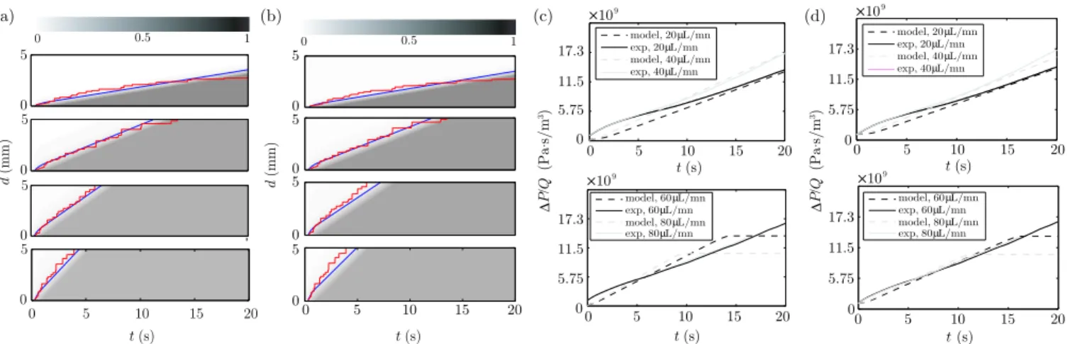
0 0.5 1 (a) 0 5.75 11.5 17.3 (c) 0 5 10 15 20 0 5.75 11.5 17.3 t(s) ∆ P / Q ( P a s /m ) 0 5 0 5 d (mm) 0 5 t(s) 0 5 10 15 20 0 5 model, 20µL/mn exp, 20µL/mn model,40µL/mn exp,40µL/mn model,60µL/mn exp,60µL/mn model,80µL/mn exp,80µL/mn 0 5 10 15 20 t(s) 0 0.5 1 (b) (d) d (mm) t(s) 0 5 10 15 20 0 5.75 11.5 17.3 t(s) model, 20µL/mn exp, 20µL/mn model,40µL/mn exp,40µL/mn 0 5 10 15 20 0 5.75 11.5 17.3 t(s) model,60µL/mn exp,60µL/mn model,80µL/mn exp,80µL/mn 0 5 0 5 0 5 0 5 10 15 20 0 5 . 3 9 10 109 ∆ P / Q ( P a s /m ) . 3 9 10 109
Fig. 6 Comparisons of front positions and flow resistance between experiments and calculations. (a) Contour plots of the calculatedφs(x, t) for varying flow rates, Q=20, 40, 60 and 80µL/min, from top to bottom. Equation 3 is used to compute
the mobility M in the calculations. The gray value at each point represents the value of φs, as indicated by the gray scale bar on the top. Red curves indicate experimentally measured front positions from figure 5. Blue curves are lines of φs = 0.1.
(b) Calculatedφs(x, t) using equation 6. (c)(d) Calculated flow resistance ∆P/Q (dashed) in comparison with the measured
resistance for different flow rates. (c)(d) correspond to (a)(b), respectively. The plateau of the dashed line in the bottom panels indicates a steady state of ∆P
Q at whichφs,max in the entire channel.
In addition to equation 3, a simpler expression, which asymptotically captures the low and highφsflow mobility
limits exactly, was used for comparison:
M = (1−φs)nM0. (6)
Here M0 is the mobility of a flow in an empty channel
φs= 0. Given the channel dimensions and the fluid
vis-cosity,M0= 3.03×10⁻⁸ m2
Pa·s can be determined analyt-ically for a rectilinear channel. The constant n is fit to the data.
To solve equations 1-2, appropriate initial and bound-ary conditions are needed forφs,φf. To reproduce
exper-iments,φf(x,0) =φf(0, t) =φf,in= 0.02 andφs(x,0) = 0
for all calculations. In addition, a constant flow rate con-straint was enforced in the calculation. The model equa-tions were solved numerically using an upwinded scheme to approximate the spatial derivatives and integrating the resulting ordinary differential equations with a forth or-der Runge-Kutta method.
Numerical Results
The calculated evolution in φs(t) are presented in
fig-ure 6(a)(b). Parameter valuesr= 33µm,P = 6 MPa/m,
α=10 s−1 and n = 6.2 were chosen for all calculations. The column radiusr used in calculations is about twice larger than the experimental one which is measured from the images of the visible columns. Considering only the columns in the region φs(x) φs,max are visible,
we expect larger column radius in the particle dense re-gionφs(x) = φs,max since coarsening process progresses
as φs(x) < φs,max. Note that τh is related to P by
Phw ∼= 2τh(h+w), in which h and w are the width
and the height of the channel36. With the fitting
pa-rameter P, we get an estimation on the yield stress
τy ∼ τh ∼ 438 Pa. The evaluated τy is about half of
the one,τy = 1000 kPa, obtained from steady shear
mea-surement for an undiluted fluid (41% v/v) operating at
E = 4 kV/mm. The discrepancy in τy might be
at-tributed to the change of particle volume fraction since the volume fraction of stuck particle φs,max in the flow
channel might be lower than the one of an undiluted fluid used in the shear measurement. Moreover, the measure-ments in different geometries, Poiseuille flow and Couette flow, might lead to a differentτy, which has been reported
in previous experiments42. As the contour maps show in
figure 6(a)(b), the calculatedφsusing Eqn. 3 and Eqn. 6
are almost identical. In agreement with the experimen-tal observation, a particle-dense region (φs(x) = φs,max)
originating at the entrance continuously expands toward the exit. Under the same electric fieldE=4 kV/mm, the expansion rate increases with flow rate, as seen in ex-periments. Since the relationship of light transmittance withφs is unknown, it is challenging to extract the front
movements from the contour map ofφs(x, t) and directly
compare them to the ones measured from experiment. To extract the front movements from model calculations, we define the front as the locations where φs(x) reaches at
a critical value. With this definition, the front motions can be traced from model calculation by finding the con-tour line ofφson the plot ofφs(x, t). We found that the
lines of φs=0.1 best fit with the front movements from
experimental measurements as shown in figure 6(a)(b). Figure 6(c)(d) also shows the calculated flow resistance
∆P
Q with a direct comparison to the experimental mea-surements. As the number of stuck particles increases, the calculated flow resistance increases over time. Us-ing either Eqn. 3 or Eqn. 6 for computUs-ing M, the cal-culated flow resistances (dashed lines) are quantitatively comparable to the measured ones (solid lines) in principle for all flow rates. However, it is also seen that calcula-tions predict a slower initial growth of ∆P
Q relative to those measured in experiments. A potential reason for the slow initial rises in calculated ∆P
Q is that the resis-tance to fluid flow that arises from particle migration to-wards walls have not been included in our simple model. In the experiments, when the field is initially applied par-ticles are dragged perpendicular to the flow direction at the onset of particle chaining. This leads to a significant disruption to the primary flow and hence a large added flow resistance. In addition to these secondary flows, the change of column radiusr during initial column forma-tion provides another possible explanaforma-tion. According to equation 4-5, the flow mobility M scales quadratically with r for constant φs. At the initial phase of column
formation, thin particle chains (one particle wide) first form upon the application of electric field and then chains merge into thicker columns. This integration process re-sults an increase ofrand thus a slowed growth in ∆P
Q at the late stage.
In addition to the discrepancy in initial growth, the calculated ∆P
Q plateaus to a steady state sooner than the experimental data (bottom plots of figure 6(c)-(d)). At this steady state, the rate at which particles are attracted to the fixed structures is equal to the one at which particle are sheared off from the structures, and an equilibrium is established between particle attaching and detaching. It is clear that the time to reach this steady state is de-termined by the expansion rate of the low-transmittance region. When the front of the low-transmittance region arrives at the exit, φs(x) =φs,max in the entire channel
and no more change in ∆QP is expected. The calculations predict a steady ∆P
Q around t=18 s and 15 s for Q= 60 and 80µL/min respectively (dashed lines). However, the steady ∆P
Q is not achieved in experiments (solid lines) within the time duration of 20 s. The postponement of the steady ∆QP in the experiment indicates that in the low-transmittance region (φs(x) =φs,max)φsis still
grow-ing but at a relatively slow rate (i.e. the growth rateαin
equation 2 is small but not zero) so that the expansion of low-transmittance region slows. This decelerated growth inφs suggests a dependence of α onφs, which we have
not captured in our simple model.
Conclusion
We have designed a microfluidic channel with conduc-tive channel walls that enables direct microscopic imag-ing of a pressure-driven ER fluid flow. With this capabil-ity we have visualized the structure evolution in a dilute ER fluid for varying flow rates Qand field strengths E. Quantitative measurement of the structure growth has been made and related to the change of flow resistance using models of flow in porous media.
For a given flow rate Qand field strengthE, there ex-ists a maximum volume fraction of particlesφs,max
incor-porated into the fibrillar structure that develops in the matrix for structure growth. When φs,max, an
equilib-rium is established between the rate of column formation and destruction. The value of φs,max can be determined
by balancing the hydrodynamic stress which exerts on the column with the yielding stress which the column can hold, Mn ∼ 1. For exact prediction of φs,max,
ex-act models for calculations of hydrodynamic stress and yielding stress are required.
The time to achieve the valueφs,maxin the entire
chan-nel is determined by two time scales. One is the time for particle polarization and aggregationta =α−1.
An-other is the convection time for sufficient particles to be delivered ta = AL(φs,max−φf,in)
Qφf,in
. The ratio of ta
tc defines
a dimensionless quantity which determines the limiting rate of structure growth and hence the time for achieving the maximum ∆P
Q . ta is typically small (∼100 ms) un-der electric fields ofE= 3−4 kV. In contrast,tccan be
very small or large, depending on the values ofQ,Land
φf,in. For fixedQandL,tc is much larger thantaat low
φf,in. So the structure growth is limited by the rate of
particle delivery and the time for achieving steady flow resistance is solely determined bytc. As φf,in increase,
tc reduces. When φf,in ≥φs,max, tc is negligible and the
structure growth is dominated by particle aggregation. For fast actuated hydraulic devices, achieving the best performance (i.e. maximum∆QP) at short times is desired and therefore the use of high volume fraction suspension is preferable.
A phenomenological model has been built for predict-ing the growth of the particle structure in the channel and the evolution in the flow resistance. By adjusting two unknown parameters, calculation using this one di-mensional model reproduces the principle experimental
observations of structure growth and predicts an increase of flow resistance. Although the calculated flow resis-tance is quantitatively comparable to experimental mea-surement, an earlier approach to the steady state for ∆P
Q is predicted by the model. In addition, there is some discrepancy observed in the initial rise of flow resistance when the porous media is very sparse. These differences reveal the complexity of the coupled interactions between particles, fluid flow and electric field, and indicate that exact models for describing these interactions are needed for precise prediction of structure growth.
Although the analysis performed in the study is for microchannel flows operating at constant flow rate, the phenomenological model can be easily adapted for flows operating at constant pressure, by changing the boundary condition at the entry. With the modified model, the performance of a realistic ER valve can be simulated with given system parameters.
Acknowledgments
We would like to thank Ahmed Helal and Maria Telle-ria for the rheological measurements of yield stress, and Marc Strauss and Mike Murphy for the construction of high voltage driver circuit. This work was supported by DARPA M3.
References
1 W. M. Winslow,J. Appl. Phys., 1949,20, 1137–1140. 2 M. Whittle, R. Firoozian and W. A. Bullough,J. Intell. Mater.
Syst. Struct., 1994,5, 105–111.
3 S. B. Choi, C. C. Cheong, J. M. Jung and Y. T. Choi, Mecha-tronics, 1997,7, 37–52.
4 D. Carlson and T. G. Duclos,Proc. 2nd Int. Conf. on ER Flu-ids, 1990, 353–367.
5 S. B. Choi, Y. M. Han, H. J. Song, J. W. Sohn and H. J. Choi, J. Intell. Mater. Syst. Struct., 2007,18, 1169–1174.
6 T. Tateishi, K. Shimada, N. Yoshihara, J. W. Yan and T. Kuriyagawa,Adv. Mater. Res., 2009,69-70, 148–152. 7 L. Wang, M. Zhang, J. Li, X. Gong and W. Wen, J.
Mi-cro/Nanolith. MEMS MOEMS, 2009,8, 021103.
8 L. Wang, M. Zhang, J. Li, X. Gong and W. Wen,Lab Chip, 2010,10, 2869–2874.
9 K. Yoshida, M. Kikuchi, J. H. Park and S. Yokota,Sens. and Actuator A: Phys., 2002,95, 227–233.
10 X. Niu, W. Wen and Y. K. Lee,Appl. Phys. Lett., 2005,87, 243501.
11 L. Liu, X. Chen, X. Niu, W. Wen and P. Sheng,Appl. Phys. Lett., 2006,89, 083505.
12 L. Liu, X. Niu, W. Wen and P. Sheng,Appl. Phys. Lett., 2006, 88, 173505.
13 W. Wen, X. Huang, S. Yang, K. Lu and P. Sheng,Nat. Mater., 2003,2, 727–730.
14 J. M. Ginder and S. L. Ceccio,J. Rheol., 1995,39, 211–234. 15 Y. Tian, Y. Meng and S. Wen,J. Intell. Mater. Syst. Struct.,
2004,15, 621–626.
16 Y. Tian, C. Li, M. Zhang, Y. Meng and S. Wen, J. Colloid Interface Sci., 2005,288, 290–297.
17 K. Tanaka, A. Sahashi and R. Akiyama,Phys. Rev. E, 1995, 52, R3325.
18 K. L. Smith and G. G. Fuller,J. Colloid Interface Sci., 1993, 155, 183–190.
19 J. M. Ginder,Phys. Rev. E, 1993,47, 3418–3429.
20 K. Tanaka, K. Nakamura and R. Akiyama,Phys. Rev. E, 2000, 62, 5378–5382.
21 J. C. Hill and T. H. V. Steenkiste,J. Appl. Phys., 1991,70, 1207–1211.
22 D. Klingenberg, C. Zukoski and J. C. Hill,J. Appl. Phys., 1992, 73, 4644–4648.
23 W. Wen, D. W. Zheng and K. N. Tu,Appl. Phys. Lett., 1998, 85, 530–533.
24 W. Wen, D. W. Zheng and K. N. Tu,Rev. Sci. Intrum., 1998, 69, 3573–3576.
25 D. Klingenberg and C. Zukoski,Langmuir, 1990,6, 15–24. 26 H. See and M. Doi,J. Rheol., 1992,26, 1143–1163. 27 R. Tao and Q. Jiang,Phys. Rev. Lett., 1994,73, 205–208. 28 R. Tao,Chem. Eng. Sci., 2006,61, 2186–2190.
29 G. Bossis, C. M´etayer and A. Zubarev,Phys. Rev. E, 2007,76, 041401.
30 S. Ulrich, G. B¨ohme and R. Burns, J. of Phys.: conf. Ser., 2009,149, 012031.
31 Y. M. Han, Q. H. Nguyen and S. B. Choi,Smart Mater. Struct., 2009,18, 085005.
32 Y. S. Jeon, Y. M. Han, Q. H. Nguyen and S. B. Choi,J. of Phys.: Conf. Ser., 2009,149, 012012.
33 E. J. Rhee, M. K. Park, R. Yamane and S. Oshima,Exp. Fluids, 2003,34, 316–323.
34 Y. J. Nam, M. K. Park and R. Yamane,Exp. Fluids, 2008,44, 915–926.
35 M. Ocalan and G. H. McKinley,J. Intell. Mater. Syst. Struct., 2011,0, 1–10.
36 Y. Son,Polymer, 2007,48, 632–637.
37 P. A. Arp and S. G. Mason,Colloid Polym. Sci., 1977, 255, 566–1165.
38 A. P. Gast and C. F. Zukoski,Adv. Colloid Interface Sci., 1989, 30, 153–202.
39 H. G. Lee, S. B. Choi, S.S.Han and J. Kim,Int. J. Mod. Phys. B, 2001,15, 1017–1024.
40 Y. T. Choi and N. M. Wereley,J. Intell. Mater. Syst. Struct., 2002,13, 443–450.
41 M. V. Bruschke and S. G. Advani,J. Rheol., 1993,37, 479–498. 42 H. G. Lee and S. B. Choi,Mater. Design, 2002,23, 69–76.