Predicting bid prices in construction projects using non-parametric statistical models

PREDICTING BID PRICES IN CONSTRUCTION PROJECTS USING NON-PARAMETRIC STATISTICAL MODELS

A Thesis by

ROSHAN PAWAR

Submitted to the Office of Graduate Studies of Texas A&M University

in partial fulfillment of the requirements for the degree of MASTER OF SCIENCE

August 2007

PREDICTING BID PRICES IN CONSTRUCTION PROJECTS USING NON-PARAMETRIC STATISTICAL MODELS

A Thesis by

ROSHAN PAWAR

Submitted to the Office of Graduate Studies of Texas A&M University

in partial fulfillment of the requirements for the degree of MASTER OF SCIENCE

Approved by:

Chair of Committee, Seth Guikema

Committee Members, Ken Reinshmidt J. Eric Bickel Head of Department, David Rosowsky

August 2007

ABSTRACT

Predicting Bid Prices in Construction Projects Using Non-parametric Statistical Models. (August 2007)

Roshan Pawar, B.E., University of Mumbai Chair of Advisory Committee: Dr. Seth Guikema

Bidding is a very competitive process in the construction industry; each competitor’s business is based on winning or losing these bids. Contractors would like to predict the bids that may be submitted by their competitors. This will help contractors to obtain contracts and increase their business. Unit prices that are estimated for each quantity differ from contractor to contractor. These unit costs are dependent on factors such as historical data used for estimating unit costs, vendor quotes, market surveys, amount of material estimated, number of projects the contractor is working on, equipment rental costs, the amount of equipment owned by the contractor, and the risk averseness of the estimator. These factors are nearly similar when estimators are estimating cost of similar projects. Thus, there is a relationship between the projects that a particular contractor has bid in previous years and the cost the contractor is likely to quote for future projects. This relationship could be used to predict bids that the contractor might quote for future projects. For example, a contractor may use historical data for a certain year for bidding on certain type of projects, the unit prices may be adjusted for size, time and location, but the basis for bidding on projects of similar types is the same. Statistical tools can be used to model the underlying relationship between

the final cost of the project quoted by a contractor to the quantities of materials or amount of tasks performed in a project. There are a number of statistical modeling techniques, but a model used for predicting costs should be flexible enough that it could adjust to depict any underlying pattern.

Data such as amount of work to be performed for a certain line item, material cost index, labor cost index and a unique identifier for each participating contractor is used to predict bids that a contractor might quote for a certain project. To perform the analysis, artificial neural networks and multivariate adaptive regression splines are used. The results obtained from both the techniques are compared, and it is found that multivariate adaptive regression splines are able to predict the cost better than artificial neural networks.

DEDICATION

Dedicated to my parents Suresh and Sharayu Pawar and brother Abhishek Pawar.

ACKNOWLEDGEMENTS

I would like to thank the committee chair Dr. Seth Guikema for providing his assistance throughout the research. I am grateful to Dr. Ken Reinshmidt and Dr. J. Eric Bickel for providing assistance during the research.

I would like to thank all the faculty members of Civil Engineering Department, Dr. Stuart Anderson, Dr. David Ford and Dr. David Trejo for providing me with valuable knowledge. I would also like to thank the Civil Engineering Department staff for their assistance in administrative matters.

I would like to thank Jeremy Coffelt for providing important information on neural networks and multivariate adaptive regression splines.

I would like to thank Hrishikesh Sharma for providing his assistance for coding in MATLAB. I would like to thank William Imbeah, Shridhar Yamijala, Neethi Rajagopalan, Seung Ryong Han and David Wolter from the Guikema Research group for providing their inputs on the thesis.

I would like to thank Ms. Mary Ellen McWhirter and the staff at Salford Systems for providing their assistance with the MARS software.

TABLE OF CONTENTS

Page

ABSTRACT ... 55Hiii

DEDICATION ... 56Hv

ACKNOWLEDGEMENTS ... 57Hvi

TABLE OF CONTENTS ... 58Hvii

LIST OF FIGURES ... 59Hix LIST OF TABLES ... 60Hx 1. INTRODUCTION ... 61H1 1.1. Background ... 62H4 1.2. Problem statement ... 63H7 2. DATA DESCRIPTION ... 64H8

3. ARTIFICIAL NEURAL NETWORKS ... 65H14

3.1. Introduction ... 66H14

3.2. Background ... 67H17

3.3. Conclusions for neural network ... 68H26

4. MULTIVARIATE ADAPTIVE REGRESSION SPLINES ... 69H29

4.1. Introduction ... 70H29

4.2. Background ... 71H30

4.3. Principal component analysis ... 72H33

4.4. Analysis using MARS ... 73H40

4.5. Results ... 74H43

5. CONCLUSION ... 75H49

Page REFERENCES ... 77H55 APPENDIX A ... 78H61 APPENDIX B ... 79H63 APPENDIX C ... 80H93 APPENDIX D ... 81H105 APPENDIX E ... 82H107 APPENDIX F ... 83H110 APPENDIX G ... 84H123 VITA ... 85H148

LIST OF FIGURES

FIGURE Page

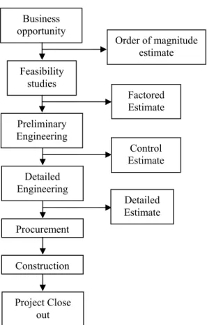
1 Estimates at various stages of a project life cycle ... 3 

2 Correction of error using target data ... 15 

3 Structural classification of neural networks ... 18 

4 Structure of neural network e.g. [1441] network ... 21 

5 Actual vs. predicted for artificial neural network with [1221] configuration .. 26 

6 Actual vs. predicted for validation set of ANN with [1221] configuration ... 27 

7 Output of neural network with data transformed using principal component analysis ... 28

8 Variance explained for the whole dataset ... 37 

9 Cumulative variance explained for the whole dataset ... 38 

10 % variance explained for the first 108 principal components ... 39 

11 Cumulative % variance explained for the first 108 principal components ... 39 

12 Actual vs. predicted for model 5 ... 46 

13 Actual and predicted bid prices for projects in validation set of model 5 ... 47 

14 Percent variation of predicted values from actual values ... 47 

15 Percent variation of actual from predicted vs. bid costs ... 48 

16 Comparison of best models from MARS and ANN ... 49 

LIST OF TABLES

TABLE Page

1 A small sample of the input data ... 102H9

2 Training and validation set statistic ... 103H11

3 Summary of different iterations for the neural network ... 104H25

4 Parameters for different model runs ... 105H44

5 MARS results ... 106H45

6 Results for CND 374 ... 107H51

7 Variation of predictions from actual for CND 374 ... 108H53

1. INTRODUCTION

Estimation of cost is carried out during various phases of construction to assess total project cost or to predict costs that may be incurred during different stages (Hendrickson and Au 1998). There are two types of estimates, as described by Faghri (2000), scratch based estimate and bid based estimate. Scratch based estimate uses information such as price, quantity, equipment, manpower and construction procedure, while bid based estimates use data available from similar projects in the past to predict the cost of the project (Faghri 2000). Hendrickson and Au (1998) has classified cost estimation based on its function into three categories viz., design estimates, bid estimates and control estimates. Design estimates are used by owners or design professionals during various stages of the design phase of the project. At the feasibility phase of the project a screening estimate (or an order of magnitude estimate) is prepared to assess the feasibility of the project, followed by a conceptual estimate which is based on the conceptual design of the facility to make a “go/no go” decision (Hendrickson and Au 1998). A detailed estimate is made when the scope of the work is clearly defined followed by an engineer’s estimate based on plans and specifications before the project is set out for bidding (Hendrickson and Au 1998). Bid estimates are prepared by contactors for the purpose of competitive bidding.

The contractor may either use quantity takeoff for this purpose or base their estimate on the work breakdown structure (Hendrickson and Au 1998). The contractor would like to invest a limited amount of effort in preparing an estimate since this effort is worthless if the work is not awarded to him (Hendrickson and Au 1998).

Cost estimates can also be based on information available from historical and prevailing unit prices of materials used in various construction activities carried out throughout the country. However, every construction project is unique, each project differs due to factors such as location, construction practices, material costs, type of materials used, labor costs, engineering and design, schedule, weather changes, taxes, inflation, budget allocations and legal requirements. Due to these variations, estimating cost of the final facility is difficult and suitable adjustments are made to the final cost estimate to incorporate these variations by including location and time adjustments, contingency, and inflation factors. The goal is to estimate the cost with reasonable accuracy by taking into consideration the sources that introduce such variability, but this is seldom possible due to the limited amount of information available on these factors.

Figure 1 shows the types of estimates prepared during the life cycle of a project. The accuracy of an estimate depends on scope definition and accuracy of information available while preparing the estimate. For an order-of-magnitude estimate, the range of accuracy is +/- 30 to 50%, for factored estimate the range of accuracy is +/- 25 to 30%, for a control estimate the range of accuracy is +/- 10 to 15% and for a detailed or definitive estimate the range of accuracy is +/- < 10% (Oberlender 2000). A statistical model to predict the total cost of a project based on historical data can be developed only

if the projects are similar in scope. In the construction industry, roads, highways, bridges, and such other projects have similar scope of work. Statistical models to predict project costs could be developed for such projects which have fairly similar scope of work for example construction of a bridge measuring certain miles in length.

Figure 1: Estimates at various stages of a project life cycle

Predicting a competitors’ bid can help a contractor adjust his bid accordingly to win a contract. Scratch based cost estimation is a tedious and time consuming process which not only requires detailed knowledge of the scope of the project but also the unit

Business opportunity Preliminary Engineering Detailed Engineering Procurement Construction Feasibility studies Project Close out Factored Estimate Detailed Estimate Order of magnitude estimate Control Estimate

cost for each activity. There is a need for a quick and reliable technique for estimating project costs. If data from previous bids about projects with similar scope of work are available, statistical models may be developed to predict final bid prices. Neural networks are one such tool that can be used in various applications for such predictions. Some of the fields where neural networks are used are predicting sales (Thiesing and Vornberger 1997), forecasting weather (Maqsood et al. 2004), hand written zip code recognition used in US Postal Service (Hassoun 1994), predicting the flow of rivers (Karunanithi et al. 1994) and pattern recognition (Basheer and Hajmeer 2000). Multivariate Adaptive Regression Splines (MARS), developed by Salford Systems, is another powerful statistical tool that is capable of developing adaptive models. The advantage of using MARS is that it is an adaptive tool that uses the data to determine the function to be fitted to segments of data. Cost estimation using historical data by these statistical models could fasten the estimation process. This process of estimating cost is data driven, when extensive data is available this process is both easy and efficient.

1.1. Background

In the construction industry, neural networks have been a topic of research in fields such as structural engineering, structural condition assessment and monitoring, construction scheduling and management, construction cost estimation, resource allocation and scheduling, environmental and water resource engineering, traffic engineering and highway engineering (Adeli 2001). Maru and Nagpal (2004) have

frames using deflections calculated from an approximate procedure. Artificial neural networks are used in diverse fields for prediction and forecasting using data depicting non-linear behavior. Li et al. (1999) used neural network to extract rules for markup estimation after training the network. Li et al. (1999) developed a neural network to predict the mark-up on estimated project cost which would also provide reasons for selecting the specified mark-up. Factors such as project size, location, market conditions, number of competitors, working cash requirements, overhead rate, contractor’s current workload, labor availability and project complexity were used for making a decision for setting up a mark-up percentage from rules extracted from trained neural networks (Li et al. 1999). Adeli and Wu (1998) used a regularization neural network to estimate unit cost for constructing a reinforced concrete pavement. Wilmot and Mei (2005) used neural networks to predict cost escalation in highway construction projects. They used data such as cost of construction materials, labor and equipment along with the characteristics of the contract to predict escalation (Wilmot and Mei 2005). Faghri (2000) used an artificial neural network to estimatetransportation project cost with data such as median unit price and the quantity of material used in projects. Neural networks have also been used to forecast escalation in construction cost using historical data available from Engineering News Record (ENR 2005) using parameters such as material, labor and equipment (Sinha and McKim 1997).

Even though a lot of research work is being done in predicting construction cost, it would be useful if it is possible to predict bids submitted by competing contractors. This may inform a contractor of his chances of winning in a competitive bidding

process. If a statistical model can be trained with data from past bids submitted by the competing contractors it may be able to predict the bids those contractors will quote in other projects.

Multivariate adaptive regression splines is a relatively new technique used for modeling data depicting non-linear relationship. Riedi (1997) has used multivariate adaptive regression splines in modeling segmental duration in speech synthesis for predicting natural sounding durations for German language. Leathwick et al. (2005) has used MARS to predict the distribution of New Zealand’s freshwater diadromous fish by determining relationship between fish species and different environmental variables. Chou et al. (2004) has used artificial neural network and MARS in developing diagnostic techniques that help in identifying breast cancer using a fine needle aspiration cytology dataset. Loizos and Karlaftis (2006) have used an artificial neural network and multivariate adaptive regression spline models for a comparative analysis of pavement condition assessment. Sephton (2005) has used MARS to find a relationship between changes in inflation and interest rate spread. Using MARS, Sephton (2005) estimated models to link changes in inflation rates over a number of policy horizons. The author concludes that tightening the yield spread will reduce inflation when the horizon of study is three to five years as opposed to a three month period.

1.2. Problem statement

The prediction of total project cost is important to determine the investment that a contractor might have to make in a project. To win a bid, a contractor should have information on the estimated cost of the project as well as the bid prices quoted by competing contractors. The aim of this research is to test different models and find out a model which may predict bid prices that other contractors may quote in certain projects. For this to be possible projects with similar scope and construction conditions are required. Highway construction projects are largely similar due to specifications and regulations in place which standardize their scope. The Tennessee Department of Transportation (TDoT) provides information about quantity for each activity performed for a project and the different tasks to be completed for the project. This information can be used to predict bids. Since the data available from TDoT has a lot of variability a statistical tool that is flexible enough to model the variability should be used to perform the analysis. Artificial neural networks and multivariate adaptive regression splines are two such non-parametric, adaptive statistical tools which are data driven. Comparison between the two models will be done using the same dataset on the basis of predicted values. If a model could predict the bid prices reasonably for each of the subcontractors participating in the bid as well as the bid a contractor should submit there would be considerable saving in time and energy in estimating the total cost of the project.

2. DATA DESCRIPTION

Data for the analysis was obtained from the website of the Tennessee Department of Transportation (TDoT 2006). The data obtained consists of highway projects undertaken by TDoT during the year 2005. The information available on the website includes a brief description of work, location of the projects, a unique identifier for each work item involved (referred to as the line item number), quantity of each line item, unit price quoted for each line item by every contractor participating in the bidding process, name of the contractors bidding for the projects and place and date when the bid was opened. Historical cost indices for the entire year are available from Engineering News Record. TDoT has divided the state of Tennessee into four regions for managing the work in each region. Data from all the four regions was used to build the model. TDoT uses unit price bidding for all their projects. The data collected contains information such as unit prices quoted by each contractor for each line item, the contractors participating in the bidding process for a certain project, amount of task performed for each line item and the total bid price quoted by each contractor. Cost indices for the analysis are obtained from Engineering News Record for each month for the year 2005 (refer: Appendix A).

The data obtained from TDoT was sorted on an Excel spreadsheet to collect together all the line items or tasks used in different projects. A standard list of line items, assigned with a uniform identification number for each line item for all the projects

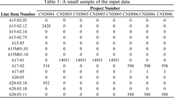
under consideration, was used to collect and group the data. Table 1 shows the format in which input was provided to the neural network.

Table 1: A small sample of the input data

Project Number

Line Item Number CND004 CND005 CND005 CND005 CND005 CND006 CND006 CND006

615-02.05 0 0 0 0 0 0 0 0 615-02.12 2428 0 0 0 0 0 0 0 615-02.14 0 0 0 0 0 0 0 0 615-02.75 0 0 0 0 0 0 0 0 615-05 0 0 0 0 0 0 0 0 615M01.03 0 0 0 0 0 0 0 0 615M01.10 0 0 0 0 0 0 0 0 617-01 0 14951 14951 14951 14951 0 0 0 617-02 518 0 0 0 0 598 598 598 617-05 0 0 0 0 0 3 3 3 620-03 0 0 0 0 0 0 0 0 620-03.10 952 0 0 0 0 0 0 0 620-03.10 0 0 0 0 0 0 0 0 620-03.11 0 0 0 0 0 588 588 588

The first column titled line item number represents a unique number which identifies the line item or task for each project. Projects below $6 million were selected for the analysis to reduce computational complexity by reducing the amount of data to be analyzed. The input vector includes quantities for the project, cost indices for the month in which the project was undertaken and a vector that identifies the contractor which bid on the project. The cost indices include construction cost index, which is comprised of common labor and wages per hour, and material cost index which covers fluctuation in the cost of cement, steel and lumber. The vector which identifies various contractors consists of a matrix of binary digits which are unique for each contractor.

The data set comprising of quantities, cost indices and contractor identifiers was then divided into training and validation set. The training set is used to train the model whereas the validation set is used to test the accuracy of the predictions obtained by using inputs from the validation set. A comparison of the predicted values from the testing process and the actual bid prices quoted by the contractors for the data used in the validation set is made to judge the accuracy of the model. The training set comprises of approximately 86% of the observations and the validation set forms the remaining 14%. The split between the training and validation set was selected at random. A random number generator was used to divide the dataset into a training and validation set.

Data was available on the TDoT website in pdf file format, tables were copied from each pdf file onto a spreadsheet. After the data was copied on the spreadsheet the data was filtered to include information that would be used for the analysis. The data was initially sorted according to project numbers, each project included information including date of opening the bid, place where the work is performed, line item number, description of line item, quantity for each line item, contractors who submitted their bid for the project and the amount bid by each contractor. In the next step, a uniform list of line items was used to sort all the activities that were performed in all the projects. Using this list all the projects were collected on a single spreadsheet, if there was an activity performed for a particular line item in a certain project the amount of that activity was included otherwise a zero was used. For example, in Table 1 for project CND004 the line item number 615-02.12 describes a prestressed concrete box beam (42” x 48”), this project requires 2428 linear feet of the prestressed concrete box beam, hence the number

2428 is included whereas line item number 620-03 which describes a concrete parapet is not included in the scope of work hence a zero is put in its place.

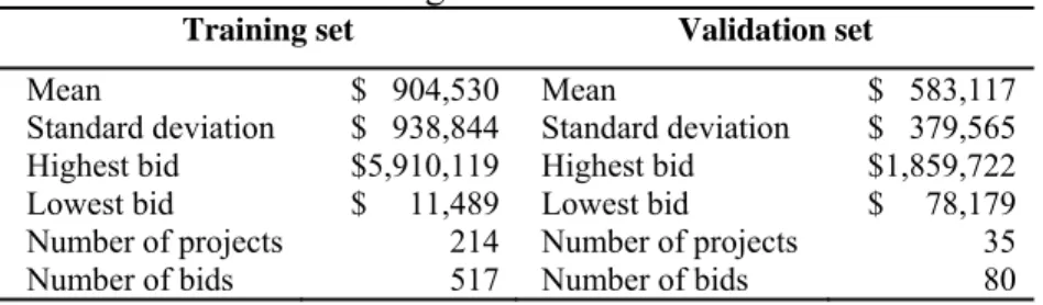
Table 2 shows statistics of the data that was used for the training and the validation set.

Table 2: Training and validation set statistic

Training set Validation set

Mean Standard deviation Highest bid Lowest bid Number of projects Number of bids $ 904,530 $ 938,844 $5,910,119 $ 11,489 214 517 Mean Standard deviation Highest bid Lowest bid Number of projects Number of bids $ 583,117 $ 379,565 $1,859,722 $ 78,179 35 80

A t-test was carried out on the means of the two datasets to compare the difference in means between the two sets. A t-test was conducted using the means and standard deviations listed in Table 2 using the following equation (Montgomery and Runger 2003): * 1 2 0 _{2 2} 1 2 1 1 0 x x t n n σ σ − − = + (2-1) where, 1

x and x₂ are the means of the training and validation sets respectively

1

σ _and σ_{2 are the standard deviations of the training and validation sets}

respectively and

n1 and n2 are the sample sizes of the training and validation sets respectively

The degree of freedom on * 0

t is calculated from the following equation (Montgomery and Runger 2003):

(

) (

)

From equation (2-1), the value of * 0

t was calculated as 3.541 and the degree of freedom (ν ) was equal to 117. Using a significance level of 0.05 and a degree of freedom of 117, the t_0.025,117 value is found to be equal to 1.981 from the t-distribution table. Since *

0

t = 3.541 > 1.981, the null hypothesis that the means are equal can be rejected and it can be concluded that the two datasets are drawn from two different populations. This conclusion suggests that a non-parametric model could be used to predict the bid costs using the given data.

The range of data for the training set is from $11,000 to $5.9 million whereas for the validation set the range of data is from $78,000 to $1.8 million. The following assumptions are made for simplification of the analysis:

1. The size of the contractors bidding on the projects has no effect on the bids submitted by them. This assumption is made because it is not possible to obtain data regarding the financial standing of the participating contractors in 2005. 2. Contract is awarded to the lowest bidder where information about winning bid is

3. Prices quoted for the materials are in accordance with the specifications provided by TDoT. This assumption is made to ensure that there is uniformity of selection of materials.

4. Contingency, profit, management fee and other overheads are included in the bid. This is assumed because the data does not indicate a separate division for such costs.

5. It is assumed that there are no delays in the projects causing cost increase and the projects have been completed successfully.

6. It is assumed that no contractor has been disqualified from the bidding process due to any reasons, this assumption is necessary because there is no information about contractors that have been disqualified from the bidding process.

3. ARTIFICIAL NEURAL NETWORKS

3.1. Introduction

According to Rumelhart et al. (1986), there are eight components of a parallel distributed processing model such as the neural network. These eight components are the processing units or neurons, the activation function, the output function, the connectivity pattern, the propagation rule, the activation rule, the learning rule and the environment in which the system operates. Neural networks are a series of interconnected artificial neurons which are trained using available data to understand the underlying pattern. They consist of a series of layers with a number of processing elements within each layer. The layers can be divided into input layer, hidden layer and output layer. Information is provided to the network through the input layer, the hidden layer processes the information by applying and adjusting the weights and biases and the output layer gives the output (Karna and Breen 1989). Each layer may have a number of processing units called neurons. The inputs are weighted to determine the amount of influence it has on the output (Karna and Breen 1989), input signals with larger weights influence the neurons to a higher extend. An activation function is then applied to the weighted inputs, to produce an output signal by transforming the input. The input can be a single node or it may be multiple nodes depicting different parameters where each of the input nodes acts as an input to the hidden layer. The hidden layer consists of a number of neurons/nodes which calculate the weighted sum of the input data. 113H

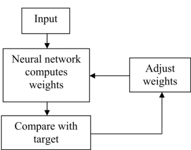
Figure 2 shows how neural network adjusts the weights and biases by comparing the output with the target. The weights are not fixed but they change over time by gaining experience after several iterations (Rumelhart et al. 1986). Artificial neural networks are used in pattern classification, clustering/categorizing, function approximation, predicting, optimization, control and content-addressable memory (Jain et al. 1996).

Figure 2: Correction of error using target data

Reference: Demuth H., Beale M., and Hagan M (2006)

Depending upon the type of input data and the output required, there are five types of activation functions used to transform input signal into output viz., linear function, threshold function, sigmoid function, hyperbolic tangent function and radial basis function. The activation functions are described briefly below:

Input Neural network computes weights Compare with target Adjust weights

Linear function: The linear function is of the type f(s) = s and is used for linear

transformation of the input. This type of activation function is used for data that have a linear relationship.

Threshold function: The threshold function is used to output a value of 1 if the value of

the function is above a threshold. For example, if st is the threshold value then for all s > st, the neural network will output a value of 1 and for all other values it will output a value of 0. The equation (3-1) shows the threshold function,

1, ( ) 0, otherwise t if s s f s _{= ⎨}⎧ > ⎩ (3-1)

Sigmoid function: The sigmoid function transforms the input into a value between zero

and one. A log sigmoid function transforms any value of the input data from + infinity and – infinity to a value between zero and one.

1 ( ) (1 exp( ) f s s ⎛ ⎞ = ⎜ _{+ −} ⎟ ⎝ ⎠ (3-2)

For the data used in this project a log-sigmoid transfer function is used in the input and intermediate layers and a linear transfer function is used in the output layer. A log-sigmoid activation function is used because it transforms any number into a value between zero and one. The equation for the log-sigmoid function is as shown in below:

1 (1 X) O e− = + (3-3)

where,

O: is the log-sigmoid transfer function.

X: is the weighted sum of the inputs from the previous layer to a particular neuron/node obtained from equation (3-3)

3.2. Background

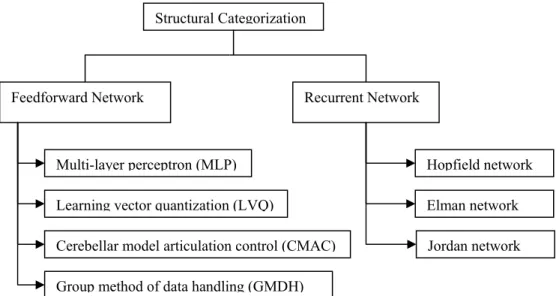
According to Pham and Liu (1995), neural networks can be categorized according to the structure and learning algorithm used. According to structure they have classified neural networks into feedforward networks and recurrent networks. Pham and Liu (1995) have classified neural networks according to the learning algorithm used into supervised learning networks and unsupervised learning networks.

In a feedforward neural network, information flows from one layer to the next from the input layer to the hidden layer and then to the output layer. The flow of information is unidirectional. The neurons in one layer are connected to the neurons in the next layer. As shown in 114HFigure 3, feedforward neural networks are further classified

into multi-layer perceptron networks (MLP), learning vector quantization networks (LVQ), cerebellar model articulation control networks (CMAC) and group-method of data handling networks (GMDH) network (Pham and Liu 1995).

Multilayer perceptron networks (MLP): A multilayer perceptron network is a neural

network with a number of layers consisting of neurons with sigmoid activation function (Pal and Mitra 1992). In a multilayer perceptron network, the information is not

exchanged within the layer but neurons from one layer are interconnected with neurons of the adjacent layers with weights determining the degree of correlation between the neurons of the adjacent layers (Pal and Mitra 1992). Multilayer perceptrons uses error back-propagation algorithm to train the network. The error back-propagation technique is a two step process, in the forward step constant weights are assigned to the nodes to compute a response, in the backward step the weights and biases are adjusted to reduce the error between the calculated response and the target values (Haykin 1994).

Figure 3: Structural classification of neural networks

Learning vector quantization (LVQ): It is a supervised learning technique in which

the input signal is classified into separate classes, these classes are based on similarity in the data structure (Haykin 1994). Vector quantization techniques are used for data

Structural Categorization

Feedforward Network

Multi-layer perceptron (MLP)

Group method of data handling (GMDH) Learning vector quantization (LVQ)

Cerebellar model articulation control (CMAC)

Recurrent Network

Hopfield network Elman network Jordan network

Cerebellar model articulation control (CMAC): It is a type of supervised learning

feedforward network which utilizes fuzzy associative memory (Pham and Liu 1995).

Group method of data handling (GMDH) network: The group method of data

handling network has a structure which produces an output which is a linear combination of two inputs (Pham and Liu 1995). For example if the inputs are x1 and x2 and the output is given by y, then the output is given by (Pham and Liu 1995)

2 2

0 1 1 2 1 3 1 2 4 2 5 2

y w= +w x +w x +w x x +w x +w x (3-4)

The GMDH network increases in size during training because in this type of network the weights are adjusted for each neuron, and at the same time, the numbers of layers are increased until required accuracy is achieved.

Hopfield network: Hopfield networks are a type of recurrent network which accepts

binary and bipolar inputs (Pham and Liu 1995). These types of network consist of a single layer of neuron which is connected to each others in a recurrent manner (Pham and Liu 1995).

Elman and Jordan networks: These networks are made up of multiple layers which are

similar to the multilayer perceptron except in addition to a hidden layer they have a special layer called context. In an Elman net, this context layer receives feedback from the output layer or from a hidden layer. In a Jordan network, the signal is send back from each neuron in the context layer to itself (Pham and Liu 1995).

Neural networks can also be categorized according to the learning methods used to train the network. The most common learning methods used are supervised learning, reinforcement learning and unsupervised learning. In the supervised learning method, the network is provided with input and output, the network adjusts the weights after comparing the results from the network with the output to minimize the error. In reinforcement learning, the network is not provided with the output but it is informed if the output is a good fit or not (Karna and Breen 1989). In the unsupervised learning method, input is provided to the network which adjusts the weights and segregates the input patterns into clusters with similar characteristics eg., the Kohonen learning algorithm (Pham and Liu 1995).

Using the three parameters viz., quantity for each line item, contractor identity matrix and cost indices, an input layer consisting of a single node was constructed as shown in Figure 4. The number of hidden layers can be varied depending upon the accuracy of the output required. The network is trained using data from the training set. This trained network is then used to simulate an output using the input data of the validation set. The output of this simulated network is a vector of predicted bid prices for the input data of the validation set.

Figure 4: Structure of neural network e.g. [1441] network

The input data was scaled down between zero and one so that it can be used as an input in MATLAB for constructing the network. Scaling down of the dataset was necessary because the inputs for neural network program in MATLAB require that the input be within the range of zero and one. The scaling down was done by subtracting each value with the minimum value of the whole dataset and then dividing this by the difference between the maximum value and the minimum value of the whole dataset.

Original value Minimum Changed Value Maximum Minimum − = − (3-5) Target values INPUT

LAYER LAYERS HIDDEN OUTPUT LAYER

w11

wji

Predicted values

Various iterations were performed by changing the number of layers and the number of neurons in each layer. A levenburg-marquardt algorithm was used for training the network. The neural network program in MATLAB uses the levenberg-marquardt algorithm to achieve numerical optimization through nonlinear least squares. The levenberg-marquardt algorithm aims to minimize the least squres error by approximating the Hessian matrix to achieve second order training speed, as follows (Demuth et al. 2006):

T

H J J= (3-6)

where,

H is the Hessian matrix and

J is the Jacobian matrix of the first derivatives of the errors with respect to the weights and biases (Demuth et al. 2006)

The gradient can be computed using the network error (Demuth et al. 2006)

T

g J e= (3-7)

where,

J is the first order derivative of the network errors with respect to the biases and weights and e is the vector of errors of the network (Demuth et al. 2006).

According to Demuth et al. (2006), this approximation of the Hessian matrix is similar to the Newton’s method (Demuth et al. 2006).

1

1 T T

k k

x ₊ =x −⎡_⎣J J+μ⎤_⎦− J e (3-8) The algorithm uses the above form to calculate the performance function. When

whereas if the value of µ is zero the equation (3-8) takes the form of the Newton’s method (Demuth et al. 2006). The Hessian matrix approximation using Jacobian transformation is used to arrive at the least squares error faster (Demuth et al. 2006).

In the neural network, the inputs to a node from the previous layer are multiplied by weights and summed as shown in equation (3-9) (Warner and Misra 1996).

1 (1 X) O e− = + _(3-9) where,

X: is the weighted sum of the inputs from the previous layer to a particular neuron/node.

wji: are the weights

xi: are the inputs from the previous layer

Since the inputs to the neural network are scaled down between zero and one, the output has to be scaled up to get the predicted bid prices. This process is reverse of the scaling down process which is done by using the equation shown below:

(

)

New value = ⎡_⎣Changed value Maximum Minimum− ⎤_⎦+Minimum (3-10) Using the method described above, a neural network using data from 214 projects was constructed and thirty five projects were used to validate the network. The network was trained using different configurations of the network and different neurons in each layer. The results from different runs of the validation set are as shown in

Appendix B and 115HTable 3. The projects that were used in the training and the validation

set are as listed in Appendix C.

The analysis was performed by changing the number of iterations also called epochs and the configuration of the network. The configuration of the network was changed by varying the number of neurons in each layer and/or changing the number of layers. For example, a [1 2 1] configuration denotes that it is a three layered network and there are 1, 2 and 1 neurons in the input, hidden and the output layer of the network respectively. 116HTable 3 shows a summary of the different iterations performed to analyze

the data. Root mean square error and coefficient of determination are the two parameters that are used to compare the models. The root mean square error is mathematically expressed as follows:

(

)

∑

The coefficient of determination is calculated from the regression sum of squares (SSR) and the total corrected sum of squares (SST). The regression sum of squares is given by 2 ˆ ( ) n R i i SS =

∑

y −y are the residuals

The total corrected sum of squares (SST) is the sum of the regression sum of squares and the error sum of squares (SSE).

T R E

SS =SS +SS (3-13)

The error sum of square is calculated as follows

2 ˆ ( ) n E i i i SS =

∑

The coefficient of determination is the ratio of regression sum of square (SSR) and the total corrected sum of squares (SST).

2 R T SS R SS = (3-15)

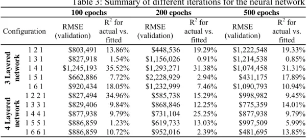
The root mean squared error and the coefficient of determination for the validation set, for different configurations of the network and for different epochs are shown in 117HTable 3. The average cost of the projects in the validation set is $583,117.

From the results it can be seen that the root mean squared error is large when compared to the average cost of the projects in the validation set.

Table 3: Summary of different iterations for the neural network

100 epochs 200 epochs 500 epochs

Configuration _(validation) RMSE R 2 _for actual vs. fitted RMSE (validation) R2 _for actual vs. fitted RMSE (validation) R2 _for actual vs. fitted 3 L ayere d network 1 2 1 $803,491 13.86% $448,536 19.29% $1,222,548 19.33% 1 3 1 $827,918 1.54% $1,156,026 0.91% $1,214,538 0.85% 1 4 1 $1,245,193 35.52% $1,293,271 31.38% $1,074,458 31.31% 1 5 1 $662,886 7.72% $2,228,929 2.94% $431,175 17.89% 1 6 1 $920,434 18.05% $1,232,999 7.46% $1,090,793 10.94% 4 L ayere d network 1 2 2 1 $827,494 34.96% $585,738 15.29% $998,982 9.45% 1 3 3 1 $829,406 9.84% $868,846 12.25% $775,359 14.01% 1 4 4 1 $877,938 9.79% $731,104 25.25% $877,938 9.79% 1 5 5 1 $886,859 1.23% $619,733 13.03% $997,509 5.99% 1 6 6 1 $886,859 10.72% $952,016 2.39% $481,695 13.85%

3.3. Conclusions for neural network

After performing different iterations, the neural network with a [1 2 2 1] configuration and 100 epochs produces the best result. It has a coefficient of determination of 0.34 and a root mean squared error of $827, 494. The plot of actual versus predicted for the neural network with [1 2 2 1] configuration is as shown in

118H

Figure 5.

Actual vs. pre dicte d plot y = 1.5151x - 101917

R2 _{= 0.3496} $0.00 $0.20 $0.40 $0.60 $0.80 $1.00 $1.20 $1.40 $1.60 $1.80 $2.00 $0.00 $0.50 $1.00 $1.50 $2.00 M illio ns Millions Actual P red ic te d

Figure 5: Actual vs. predicted for artificial neural network with [1221] configuration

Figure 6: Actual vs. predicted for validation set of ANN with [1221] configuration

119H

Figure 6 shows the ability of the network to predict most of the values for the project except a few projects. Projects number CND055 (3 and 4), CND284 (52, 53, 54 and 55) and CND334 (62) are over estimated by the neural network and these values skew the root mean square values. The average predicted error for the neural network with [1221] configuration is 141%. Though some of the values are close to the actual, there is a lot of variation in the predicted values. The actual and predicted values for neural network with [1221] configuration are as shown in Appendix D. The usefulness of the model developed by neural network can be judged only after comparing it with the model obtained from MARS.

The data transformed using principal component analysis (explained in the next section) was used to train neural network, the results obtained were not promising.

Figure 7 shows the output of the analysis using dataset transformed by principal component analysis. All the predicted values were similar to each other hence further analysis using data transformed by principal component analysis was not done.

Figure 7: Output of neural network with data transformed using principal component analysis

4. MULTIVARIATE ADAPTIVE REGRESSION SPLINES

4.1. Introduction

Multivariate Adaptive Regression Splines (MARS) is an adaptive modeling process popularized by J. H. Friedman for non-linear relationships. The modeling technique expands product spline basis functions by selecting the number of basis functions, the locations of the knots and the degrees of freedom automatically depending upon the data (Freidman 1995). The aim of the model is to capture the relationship between the dependent variable and the independent variable from the data. According to Leathwick et al. (2005), MARS divides the predictor variables into piece-wise linear segments to describe non-linear relationships between the predictor and the dependent variable.

The MARS software developed by Salford Systems was used and the results were compared with the results obtained from neural network. The MARS software automatically develops and adjusts the model by comparing the target values and the dependent variables supplied as input to the model. This is done by selecting the appropriate variables that contribute to the model fit, determining the degree of interaction between the predictor variables and conducting tests to avoid over fitting to the dataset (MARS 2001). The MARS software has a number of input/output options and is available with a graphical user interface. The data set can be entered in a number of file formats. The problem faced in fitting a model to the dataset is the type of function that will best fit to it. This problem is overcome by MARS by fitting piecewise linear

basis functions to small segments of the dataset. The other advantage of the MARS model is that it is adaptive, meaning that the model chooses the locations of the knot points depending upon several strategies. One such strategy is minimization of the least squares criterion given in equation (4-1) (Friedman and Roosen 1995),

2 ( ) 1 0 ( ) K q N q i k k i k y + a B x = = ⎡ ₋ ⎤ ⎢ ⎥ ⎣ ⎦

∑

∑

a represents the coefficient of expansion

( )q _{( )} k

B x are the basis functions that are selected for inclusion in the model of order q

4.2. Background

The aim of any regression model is to derive a relationship between the independent variables and the dependent or the predictor variables. A simple linear regression model takes the form given in equation (4-2).

i 0 1 1 2 2

y =β +β x +β x +...+β_{n n}x +ε (4-2) In equation 4-2, the β’s are called regression coefficients and ε is the error term. The x’s are the independent variables and the y’s are the dependent variables whose values can be estimated using the predictor also known as independent variables. In a MARS model the range of x values are divided into disjoint regions separated by “knot” points (Friedman and Roosen 1995). According to Friedman and Roosen (1995), a qth

degree polynomial is then fitted separately and locally to these disjoint regions and each of the qth order polynomials are then adjusted to fit the disjoint regions locally while satisfying the least squares criterion. Thus, the basis functions are used to determine a relationship between the dependent and the independent variables (Friedman and Roosen 1995). The model iteratively decreases the average squared error, shown in equation (4-3) by attempting to make the predicted values close to the actual values.

2 1 ( ) n i i i y y mse n = − =

∑

In equation (4-3), the average sum of squared error term (mse) can be minimized if the values of yi are close to ŷi. This minimization problem is converted into an

optimization problem by choosing basis functions of the form ( )q _{( )} k

B x for each of the disjoint sets between the knot points (Friedman and Roosen 1995). A linear least squares fit is then performed on each of these basis functions (Friedman and Roosen 1995). The expansion in the piece-wise linear basis function are of the form (x – t)+ and (t – x)+,,

where + signifies that the equation retains positive values (Hastie 2001). This linear basis function is of the form (Friedman and Roosen 1995)

0 ( ) ( ) k q k _q k k x t x t x t x t + ≤ ⎧⎪ − _⎨ − > ⎪⎩ (4-4)

Knots are selected adaptively in a forward/backward stepwise selection approach. A large number of knot locations are selected for the dataset during the forward selection and deleted or retained, depending upon the least squares criterion, in the backward selection process. The advantage of the adaptive knot selection process is

that outliers in the independent variables affect the model locally and there is minimal affect on the overall model (Friedman and Roosen 1995).

After the knot locations are selected, the MARS algorithm selects a number of basis functions with the aim to overfit the data. The splines for the disjoint regions separated by knots are tensor products of the splines over the independent variable (Friedman and Roosen 1995). Basis functions are selected locally, depending upon the variable and the contribution of the variable to the overall fit, the basis function is then either retained or deleted to improve the overall fit of the model. The selection of the basis function is a two step process, in the forward stepwise selection a large number of basis functions are selected (Friedman and Roosen 1995). According to Friedman and Roosen (1995), the forward stepwise process is a recursive process and at each step new two basis functions are introduced into the pool of previously entered basis functions. Interactions can be allowed between each of the basis function or for selected variables depending upon the underlying knowledge of the variable. The basis functions selected in the forward step are compared to each other depending upon some lack of fit criterion such as cross-validation. The MARS algorithm uses generalized cross-validation for pruning until the best fit model is obtained. The data used for comparing the lack-of-fit is required to be independent of the training data hence sample reuse techniques such as the cross validation technique or bootstrapping technique is used for comparing the model fit (Friedman and Roosen 1995).

The MARS algorithm implemented by Salford Systems uses the following equation proposed originally by Craven and Wahba for comparing the fit (Friedman 1991) 2 2 1 1 _ˆ ( ) ( ) N _{i M}( ) / 1_i i C M GCV M y f x N = N ⎡ ⎤ ⎡ ⎤ = _⎣ − _⎢ − _⎥ ⎦ ⎣ ⎦

∑

M : number of non constant basis functions

ˆ ( )M i

f x _{: is the model of the M basis function considered for deletion during the}

backward step

C(M) : is the cost complexity of the model and is given by C(M) = M.(d/2 + 1) + 1 and

d : smoothing parameter

The MARS program however accepts a maximum of 8019 variables hence it was necessary to reduce the dataset. To reduce the dataset and at the same time to retain the variability in the original dataset principal component analysis was used which also makes the dataset uncorrelated. Principal component analysis is discussed in the next section.

4.3. Principal component analysis

The data set from TDoT was found to be correlated. Due to computational constraints the amount of data to be analyzed was required to be reduced. Principal

component analysis (PCA) reduces the dataset while retaining most of the variability and at the same time makes the transformed data uncorrelated. Principal component analysis was performed on the whole dataset. Principal component analysis finds orthogonal linear combinations of the original dataset which have the largest variance and at the same time can be used to reduce the dimensionality of the dataset (Fodor 2002). Fodor (2002) has expressed the independent variables as

1

( ,..., )T

p

x= x x (4-6)

whose mean values are given by,

1

( ) ( ,..., _p)

E x = =μ μ μ (4-7)

The covariance matrix for the data can be represented as (Fodor 2002),

[( )( ) ]T

p p

E _× =E x−μ x−μ (4-8)

and its lower dimension or principal components (pc’s) are represented by,

1

( ,..., )T k

s= s s (4-9)

where k ≤ p

Let μi and σi denote the mean and the standard deviation of the ith observation,

such thatσ_i = Σ_{( , )i i} . The observations are standardized in order to transform the variables with different units to a set of variables that have zero mean and unit standard deviation (Fodor 2002). The sample mean ( ˆμ_i) and the standard deviation ( ˆσ_i) are given as (Fodor 2002),

( )

∑

(

)

∑

The data is standardized using the mean and the standard deviation as follows (Fodor 2002):

(

)

The principal components are linear combinations of the original variables (Fodor 2002), ,1 1 ... , i i i p p s =w x + +w x (4-13) for i = 1,……,k and k ≤ p or s Wx= (4-14)

Principal component analysis arranges the transformed variables in descending order of variance with the first few principal components explaining hopefully most of the variability. Mathematically, Fodor (2002) expresses the first principal component as follows:

1 1

T

s =x w (4-15)

(

)

1 1,1 ... 1, T p

w = w + +w (4-16)

and ₁ arg max ₁

( )

w

w = ₌ Var x w (4-17)

The second principal component explains the second largest variance and is

orthogonal to the first principal component (Fodor 2002). Thus a number of principal components are computed which retain the variance of the original data and at the same time reduces the size of the dataset. The data is standardized to have a mean zero and standard deviation of one so that they are comparable even when the variables have different units (Fodor 2002). After the data is standardized the covariance matrix can be given by (Fodor 2002),

1 T

pxp XX n

Σ = (4-18)

According to Fodor (2002), ∑ can be written using the spectral decomposition theorem as follows: T U U Σ = Λ (4-19) where, 1 ( ,..., _p) diag λ λ

Λ = is the diagonal matrix of the eigenvalues such thatλ_p ≥...≥λ₁and

U is the orthogonal matrix containing the eigenvectors.

The p rows of the p x n matrix S, in the equation below, gives the principal components (Fodor 2002).

T

S U X= (4-20)

The eigenvalues are the variances and the eigenvectors are the loadings. MATLAB was used to perform the transformation into principal components. 120HFigure 8

shows the variation explained after principal component analysis is performed on the entire dataset. 121HFigure 9 shows the cumulative percentage of variation explained.

Principal Component Analysis - % Variance explained

0 2 4 6 8 10 12 14 1 201 401 601 801 1001 1201 1401 Transformed Covariates P erc en t va ri at ion e xpl ai ne d

0 20 40 60 80 100 120 1 201 401 601 801 1001 1201 1401 Cum ul at ive % va ri at ion expl ai ne d Transformed Covariates

PCA - Plot of cumulative % variance explained

Figure 9: Cumulative variance explained for the whole dataset

Only those principal components that explain 90 percent of the variability are retained for further analysis. The first 108 principal components explain 90 percent of the variability in the whole dataset hence they are used for analyzing using multivariate adaptive regression splines. The components that explain 90 percent of the variability are retained because after this value the percentage variation explained is very small and does not change substantially.

Principal Component Analysis - % Variance explained 0 2 4 6 8 10 12 14 1 13 25 37 49 61 73 85 97 109 Transformed Covariates Pe rc en t v ar ia tion e xpl ai ne d

Figure 10: % variance explained for the first 108 principal components

PCA - Cumulative plot

0 10 20 30 40 50 60 70 80 90 100 1 13 25 37 49 61 73 85 97 Transformed Covariates Cum ul at ive % va ri at ion e xpl ai ne d

Figure 11: Cumulative % variance explained for the first 108 principal components

Figure 10 and Figure 11 shows the plot of percent variation explained and cumulative percent variation explained for the first 108 principal components.

4.4. Analysis using MARS

The dataset used for training and validation using MARS is the same as that used for analysis using artificial neural networks, except the data used for MARS was transformed using principal component analysis and only the first 108 principal components were retained. The same dataset was used so that comparison between the results using the two methods could be made. Several trials were done by fitting different models by changing various parameters, to the training set and then validating the results. The parameters were changed depending upon the results obtained by testing previous models. Models were fitted by changing certain parameters (discussed below) of the program and comparing the results for the validation set using root mean square error and plotting the predicted values against the actual values. The parameters that were varied are speed factor, penalty on added variable, maximum number of basis functions, maximum interactions, records to process, minimum observations between knots and degree of freedom. These parameters are discussed below:

Maximum number of basis functions: MARS initially constructs a number of models

in a bid to over fit the data. The number of models to be fitted is dependent on the number of basis functions allowed. It is advised to have the number of basis functions equal to two to four times of the number of predictors (MARS 2001). The number of basis function is a user specified parameter and affects the speed of the MARS run

(MARS 2001). The maximum number of basis functions is varied from 15 to 200 while performing different iterations.

Penalty on added variables: This parameter directs the MARS model to reuse the

available variables i.e. MARS will increase the number of knots for the existing variables or increase interaction between the already present variables rather than generating new variables from combination of the variables already present in the model (MARS 2001).

Minimum number of observations between knots: This parameter allows the user to

specify the number of data points between adjacent knots. By default, MARS will generate knots at every observed data point. The default setting allows MARS to select knots depending upon the data (MARS 2001). Increasing the distance between the knots will make the model more global in nature rather than being locally adaptive (MARS 2001).

Speed factor: The speed factor can be adjusted on a scale of one through five, five being

the fastest. A speed of one makes the model slower but improves the accuracy of the model. At a speed of one, MARS does intensive search of all the basis functions and chooses the one which contributes the most to the least squares criterion or any other criterion used for evaluating model fit.

Records to process: The records to process option specifies the percent of original data

that the program can process, if the option is set to zero it will process the entire dataset, if the option is set to a specific number, the program will process the specified number of observations (MARS 2001).

Maximum interactions: This setting allows the user to specify the amount of

interaction between the variables of the model. A value of one for the interaction terms makes the model additive, a value of two allows two way interaction and a value of three or more specifies that the model can be a product of one or more basis functions (MARS 2001).

Degree of freedom: The degree of freedom allows the user to impose a penalty to the

knot selection process to avoid over fitting the model to the data. Three methods are available to select the degree of freedom they are: setting it to a particular value, determining by x – fold cross-validation and by using a test sample randomly set aside from every nth _{observation. Using the first option the user can set the degree of freedom}

to a particular number, the default is set to 3.00 but it can be set to as high as 200 (MARS 2001). The second option allows the MARS model to select the degree of freedom by fold cross validation, for example if a value of 10 – fold cross-validation is specified, MARS will compute ten more models to optimize the knot selection process. In the third option, the program will set aside a randomly selected sample after every nth

4.5. Results

Different models were run by varying the parameters described above. The configurations of the different runs are as shown in 124HTable 4. The parameters were

changed depending on results obtained from previous runs. Of the thirteen different models developed, three models showed substantially good results. The results of the different runs are compared using root mean square error and coefficient of determination.

Different models were developed by changing the speed factor, penalty on added variable, maximum basis function, maximum interactions allowed, minimum observations between knots and degree of freedom. The initial model were analyzed using low values for each case, in the first three set of models the number of interactions were changed steadily while keeping the maximum number of basis functions constant. In these three models the penalty on added variable was changed to see if there was any difference in the output. The testing method for determining degree of freedom was kept constant but the value was changed in the third model (Table 4). It was observed that changing the degree of freedom affected the model. Hence, the method of determining degree of freedom was changed in subsequent iterations. It should be noted that changing the method of determining the degree of freedom to “X – cross-validation” gives better results. Other parameters that affected the model significantly are number of maximum basis function and maximum number of interactions. The model prediction improves by increasing the maximum number of basis functions and the number of

interactions. MARS selects the degree of freedom by using a generalized cross validation (GCV) criterion as discussed before. There are three methods used to determine the degrees of freedom and the “x-fold cross validation” method is the most effective method that improves prediction for this dataset.

Table 4: Parameters for different model runs

Options and Limits Testing

Model Speed factor Penalty on added variable Max. basis functions Max. Interac tions Records to process Min. observations between knots

Select method for determining degree of freedom Set to X - fold Cross validation Use test sample randomly set aside at every nth observation Model 1 4 None 15 1 0 0 3.00 - - Model 2 1 Moderate 15 2 0 0 3.00 - - Model 3 1 Heavy 15 3 0 2 4.00 - - Model 4 1 Heavy 20 10 0 0 - 10 - Model 5 1 None 100 50 0 0 - 110 - Model 6 1 None 100 100 0 0 - 10 - Model 7 1 Heavy 200 200 0 0 - 10 - Model 8 4 None 50 100 0 0 3.0 - - Model 9 1 None 100 100 0 50 - 10 Model 10 1 Moderate 50 50 0 0 - - 2 Model 11 1 None 100 100 0 110 - 110 - Model 12 1 None 110 110 0 0 - 110 - Model 13 1 None 200 200 0 0 - 500 -

The results from the models developed using the different parameters are as shown in 126HTable 5. Model number 5, 12 and 13 have R-square values of 58.27%, 42.53%

(Figure 12) shows that the MARS program is able to capture the variability in the data set reasonably well. Model number 5 has the best R-square value of 58.27% while model number 6 has the lowest root mean square error of $1,342,011.

Table 5: MARS results

127H

Figure 12 and 128HFigure 13 show the plots of the actual and the predicted for the

validation set of model 5. The predicted values for model 5 are close to the actual values for the projects in the validation set. The output from the MARS program for model 5 is attached in Appendix G. The level of accuracy achieved depends on the size of the project, the number of contractors participating in the bidding process, the type of project and the total project cost. The predictions from MARS can be improved by providing more information about the location, the total number of projects performed

Model # RMSE Coefficient of determination (R2) Model 1 $ 2,535,132 16.78% Model 2 $ 1,555,689 18.57% Model 3 $ 1,651,545 23.95% Model 4 $ 1,489,013 16.68% Model 5 $ 2,157,533 58.27% Model 6 $ 1,342,011 13.62% Model 7 $ 1,162,633 16.94% Model 8 $ 6,258,412 17.99% Model 9 $ 2,859,332 14.56% Model 10 $ 1,340,552 6.67% Model 11 $ 4,593,369 13.86% Model 12 $ 1,642,966 42.53% Model 13 $ 2,467,507 54.17%

by each contractor bidding on the project, the revenue earned by each contractor, the expected duration required to complete the project etc.

Actual vs. Predicted y = 0.7777x + 166507 R2 _{= 0.5827} 0 0.5 1 1.5 2 2.5 0 0.5 1 1.5 2 Mill ions ( $) Millions ($) Actual Pred ic te d

Figure 12: Actual vs. predicted for model 5

The average percent variation of the predicted values from the actual is about 43% with the lowest variation of 0.23% and a highest variation of 217.8%. 129HFigure 14

shows the plot of the percent variation of the predicted values against the actual values. Figure 15 shows the percent variation of the actual bid prices from the predicted values plotted against the actual bid prices.

Actual and predicted bid prices $0.00 $0.50 $1.00 $1.50 $2.00 $2.50 1 4 7 10 13 16 19 22 25 28 31 34 37 40 43 46 49 52 55 58 61 64 67 70 73 76 79 Millio ns Projects Pr o je ct bi d pr ic es ($ ) Actual values Predicted values

Figure 13: Actual and predicted bid prices for projects in validation set of model 5

0 50 100 150 200 250 0 20 40 60 80 100 % Projects

Percent variation from actual

% variation from actual

Percent variation from actual vs. actual bid cost 0.00% 50.00% 100.00% 150.00% 200.00% 250.00% $- $500,000 $1,000,000 $1,500,000 $2,000,000 Actual %

% variation from actual

5. CONCLUSION

130H

Figure 16 shows the comparison of the best models obtained from both the methods i.e. MARS and ANN with the actual values. The values obtained from MARS are closer to the actual values than those obtained from ANN.

Comparison of the best models of MARS and ANN

$-$0.50 $1.00 $1.50 $2.00 $2.50 $3.00 $3.50 $4.00 $4.50 $5.00 1 5 9 13 17 21 25 29 33 37 41 45 49 53 57 61 65 69 73 77 Mi llions Projects ($) Actual MARS ANN

Figure 16: Comparison of best models from MARS and ANN

Bid prices for some of the projects are predicted higher than the actual values by the MARS and ANN model. This is a major drawback of both the models because if the predicted values are higher than the actual values quoted by other contractors, the contractor might lose the contract. If all the contractors bidding on a project use this model to predict the bid prices, then every contractor will know what the other contractors are going to quote on the project. This situation is a problem of decision