Title: Lighting the black box: explaining individual
predictions of machine learning algorithms
Author: Pol Ferrando Hernández
Advisor: Pedro Delicado Useros, Lluís Belanche Muñoz
Department: Estadística i Investigació Operativa
University: UPC-UB
Academic year: 2017-2018
Interuniversity Master
in Statistics and
Operations Research
UPC-UB
Universitat Polit`
ecnica de Catalunya
Facultat de Matem`
atiques i Estad´ıstica
Master Thesis (MESIO)
Lighting the black box: explaining individual
predictions of machine learning algorithms
Pol Ferrando Hern´
andez
Advisors: Pedro Delicado Useros, Llu´ıs Belanche Mu˜
noz
First and foremost, I would like to express my
sincerest gratitude to my advisors, Dr.
Pe-dro Delicado Useros and Dr. Llu´ıs Belanche
Mu˜noz, for the continuous support. Their
guid-ance helped me in all the time of research and writing of this thesis. Finally, I also dedicate it to my family, that always believe in me and made me who I am today.
Abstract
Keywords: machine learning, interpretability
MSC2000: 200068T01
Many machine learning techniques remain “black boxes” because, despite their high predictive perfor-mance, it is difficult to understand the role of each variable involved in the prediction task and how it combines with others to produce a prediction. In this thesis, we have studied in depth and unified the no-tation of three methods found in the literature that can explain individual predictions of any model: Local Interpretable Model-agnostic Explanations (LIME), explanation vectors and Interactions-based Method for Explanation (IME). These methods determine what explanatory variables are most influential for each par-ticular observation, which provides understanding of the reasons behind the model’s decision for a parpar-ticular instance and brings transparency to machine learning algorithms. In addition, we have applied these methods to an artifficial data set for which we know the role of each feature beforehand in order to analyze the strengths and weaknesses of each one of the explanation methods, compare their explanations for the same predictions and determine if the analyzed explanation methods really provide useful explanations of the reasons behind a model’s decisions. Finally, we have explored their usefulness in comparing predictions of different models.
Contents
Introduction 1
Part 1. Explanation methods 3
Chapter 1. Preliminaries 5
Chapter 2. Local Interpretable Model-agnostic Explanations (LIME) 7
1. Intuition behind LIME 7
2. Basic Concepts 7
3. Method 9
4. Sparse Linear Explanations 10
Chapter 3. Explanation vectors 15
1. Intuition behind explanation vectors 15
2. Method for classification 15
Chapter 4. Interactions-based Method for Explanation (IME) 19
1. Intuition behind IME 19
2. Cooperative game theory 19
3. Method 20
4. Example 22
Part 2. Experiment 25
Chapter 5. Cylinder in a cube 27
1. Description 27 2. Methodology 27 3. Explaining predictions 28 4. Comparing methods 36 5. Comparing models 37 Conclusions 41 References 43 Appendix A. R code 45 i
Introduction
Despite their high predictive performance, many machine learning techniques remainblack boxes because it is difficult to understand the role of each feature and how it combines with others to produce a prediction. However, users need to understand and trust the decisions made by machine learning models, especially in sensitive fields such as medicine. For this reason, there is an increasing need of methods able toexplain the individual predictions of a model, that is, a way to understand what features made the model give its prediction for a specific data point. Furthermore, this instance-based point of view allows detecting local peculiarities that could be unperceived in a global view (for example, due to cancellation effects).
A popular approach to this explanation problem is to use aninterpretable(ortransparent) model, from which an explanation can be extracted by observing its components. For instance, a decision tree can be explained by observing the rules that lead from the root to the leaves, or a generalized linear model can be explained by each feature’s estimated coefficient. Interpretable models are a valid solution (and will provide meaningful insights) as long as they are accurate for the task, but limiting ourselves to this kind of models is too restrictive and it can compromise accuracy, so it is preferrable to be able to use models as flexible as needed by the problem, without restrictions.
For less transparent models (i.e, black boxes), an alternative approach is to usemodel-specific(or model-dependent) explanations, that is, explanation methods designed specifically for a certain type of model. For example, according to [6], Breiman provided additional tools for explaining the decisions of random forests, and a lot of work has been done on explaining the decisions of artificial neural networks. The problem of these methods is that the explanation method has to be replaced every time that the model is replaced with one of a different type and, consequently, the final user needs additional time and effort to get used to the new explanation method.
Therefore, we need model-independent (or model-agnostic) explanations or, in other words, a method that can explain the predictions ofanymodel. With such explanations, we are not restricted to a specific type of model. Also, since such method uses the same techniques and representations to explain predictions of any model, it is easier to compare two candidate models for the task or to switch models if they are from different types.
The challenges for model-independent explanations are:
• Type of task. Supervised learning includes classification and regression. The question is: can an explanation method work for both type of tasks? That is, in addition to be model-independent, it would be nice to have a “task-independent” method or, at least, two versions of the method which share its essence.
• Interpretability. Even if a coefficient for each feature can be inspected, explanations can be not interpretable. For example, even a linear model can be difficult to interpret if it has hundreds or thousands of coefficients. The same happens if the input variables for the model are difficult to understand because explanations in terms of these variables will not be interpretable by a human and, consequently, they will be useless.
2 INTRODUCTION
• Locally faithful. If the explanation is generated by approximating the original black box model, we have to ensure that the approximated model behaves similarly to how the original model does in the vicinity of the instance being predicted to properly capture the relationship between the input variables and the response.
• Efficiency. Users often need to understand more than a single prediction, specially if their goal is to decide trusting a model or not. Therefore, the explanation method cannot be too computationally expensive.
• Global understanding. It would be very interesting if individual predictions (local view) can help to trust a model as a whole (global view).
• Actionability. If we can obtain a global understanding of a model with explanations, can these explanations be useful to improve the original model (by feature engineering or feature selection, for instance)?
This thesis has been developed with several objectives. First, we want to introduce the model-independent methods proposed in the literature that are able to explain individual predictions of machine learning models. Second, this work wants to unify the notation of these methods to make the comparison between them easier. Third, we want to apply these methods to a data set in order to analyze the strengths and weaknesses of each one of the chosen methods and, also, compare their explanations for the same predictions. Finally, the main goal of this project is to determine if the analyzed explanation methods really provide useful explanations of the reasons behind a model’s decisions.
The remaining part of this work is organized as follows. There are two parts: part 1 develops the theoretical framework of model-independent explanation methods and part 2 covers the experimental part. In chapter 1, we introduce basic concepts and notation that we need to describe the three considered explanation methods in chapters 2, 3 and 4. In chapter 5 we apply the explanation methods to a simple dataset for which we have previous knowledge of the role of each explanatory variable. In the end, the conclusions of the thesis are described and future work that would complement this study are discussed.
To finish this introduction, I would want to explain my personal motivation to choose this subject as a master thesis. I am interested in both machine learning and data mining, but there are some machine learning techniques that are opaque and it is difficult to extract meaningful insights from them. Consequently, I chose this topic to learn more about methods that bring transparency to machine learning models.
Part 1
Chapter 1
Preliminaries
Data are essential in statistical modeling and machine learning. Specifically, the goal of supervised learning is to predict the value of an outcome measure based on a number of input measures. These input measures that we observe are calledfeatures1, and the space where they are placed is called the feature space.
Definition 0.1. Feature space
The feature spaceX is the cartesian product ofpfeatures.
X =X1×X2×...×Xp We will often considerX =Rp.
Supervised learning algorithms try to find a useful approximation (a model) to the underlying function that determines the relationship between the features and the responses, in the sense that the model is able to properly predict the outcome for unseen instances. To do so, methods learn from a set of examples for which both features and outcome have been measured, known as training data. Furthermore, we distinguish two types of predicting tasks depending on the type of the output: classification tries to predict categorical outputs, while regression attempts to predict quantitative outputs.
Definition 0.2. Classification model (or classifier)
Let{1, ..., C}be a finite set of class labels. A classifierf = (f1, f2, ..., fC) is a mapping from a feature space to aC-dimensional space
f :X →[0,1]C such that C P c=1 fc(x) = 1, ∀x∈ X.
In classification, there are two types of classifiers: hard classifiers, which directly predict the class label of observations, andprobabilistic(or softclassifiers), whose outputs can be interpreted as probabilities. Note that Definition 0.2 includes hard classifiers when we consider that the component of the predicted class is 1 and the rest are 0.
Definition 0.3. Regression model
A regression modelf is a mapping from a feature space to the real numbers
f :X →R
In addition to predictive accuracy, which is not the focus of this work, an important part of data analysis is to gain insights into the underlying function that determines the relationship between the
1Also known asinputs,predictors,dependent variablesorexplanatory variables, specially in statistical literature. 5
6 1. PRELIMINARIES
features and the responses. As discussed in the introduction (see Section ), there are models inherently interpretable whose components can directly provide this understanding. However, many machine learning techniques (e.g., support vector machines or artifficial neural networks) are less transparent in this aspect and it is not clear what features are more influential on the model’s decision, which is the reason why they are calledblack boxes.
For these black box models, explanation methods try to provide qualitative understanding on what input features made a model give its prediction for a particular instance. Therefore, explanation methods assume that the user already has access to a trained modelf and one observation ˜x∈ X
whose prediction wants to be justified. Furthermore, this work focuses on model-independent methods, which do not make any assumption aboutf, so our goal is to produce an explanation for a prediction only using the predictions made by the model.
Finally, the explanation methods discussed in this work will highlight the most influential features on the model’s prediction and show them with visual artifacts to facilitate interpretability. However, it is important to keep in mind that their goal is to explain the prediction made by an specific model, so the generated explanation will be determined by the model. Consequently, on the one hand, these methods will provide meaningful insights if the model has really captured the relationship between the predictors and the outcome. On the other hand, if the model is inaccurate, explanation methods will make the user notice that the model prediction is not reliable and that the model needs to be checked in order to be trustworthy.
Chapter 2
Local Interpretable Model-agnostic
Expla-nations (LIME)
1. Intuition behind LIME
LIME (see Ref. [1] and [2]) stands for Local Interpretable Model-agnostic Explanations, a name that perfectly summarizes the three basic ideas behind this explanation method: model-agnosticism, interpretabilityandlocality.
First, LIME do not make any assumptions about the black-box model because its purpose is to be model-independent (or model-agnostic, as Ribeiro et al. say). Consequently, the only way that LIME has to understand the black-box’s behavior is perturbing the input and see how the predictions change.
Second, Ribeiro et al. argue that, for the benefit of interpretability, the input variables used to produce explanations may need to be different from the actual features used by the model. According to them, explanations have to provide qualitative understanding of the relationship between the input variables and the response, but they have to be easy to understand by users above all, which is not necessarily true of the feature space used by the model as we have seen in section??. For this reason, LIME’s explanations use a data representation (calledinterpretable representation) that is different from the original feature space.
Finally, according to LIME’s authors, it is much easier to approximate a black-box model by a simple model locally (i.e., in the neighborhood of the instance we want to explain) rather than approximate it globally. For this reason, LIME produces an explanation by approximating the black-box model by an interpretable model (for instance, a linear model with a few non-zero coefficients) learned on perturbations of the original instance weighted by their similarity to it.
In summary, LIME generates an explanation for a prediction from the components of an inter-pretable model (for instance, the coefficients in a linear regression) which resembles the black-box model at the vicinity of the point of interest and which is trained over a new data representation to ensure interpretability.
2. Basic Concepts
2.1. Interpretable representation. To ensure that the explanation isinterpretable, Ribeiro et al. (see Ref. [1] and [2]) distinguish aninterpretable representationX0 from theoriginalfeature spaceX
that the model uses.
8 2. LOCAL INTERPRETABLE MODEL-AGNOSTIC EXPLANATIONS (LIME)
The interpretable representation has to be understandable to humans, so its dimension is not necessarily the same as the dimension of the original feature space. Letp be the dimension of the original feature spaceX and letp0 be the dimension of the interpretable spaceX0.
The interpretable inputs map to the original inputs through a mapping functionhx˜:X0→ X (see
Reference [?]), specific to the instance ˜xwe want to explain. Different types of mappings are used for different input spaces.
For text data, a possible interpretable representation is a binary vector indicating the presence or absence of a word, although the classifier may use more complex and incomprehensible features such as word embeddings. Formally,X0={0,1}p0 ≡ {0,1} × · · · × {0,1}
| {z }
(p’)
wherep0 is the number of words
that contains the instance being explained ˜xand the mapping function converts a vector of 1’s or 0’s (presence or absence of a word, respectively) into the representations used by the model: if it uses word counts, the mappinghx˜ will map 1 to the original word count and 0 to 0; but if the model uses
word embeddings, the mapping should convert any sentence expressed as a vector of 1’s and 0’s into its embedded version.
For images, a possible interpretable representation is a binary vector indicating the presence or absence of a set of contiguous similar pixels (also called super pixel). Formally,X0={0,1}p0 wherep0
is the number of super pixels considered, usually obtained by an image segmentation algorithm such as quick shift (see Figure 1 for an example). In this case, the mapping function maps 1 to leaving the super pixel as in the original image and 0 to gray the super pixel out (which represents being missing).
Fig. 1. Original representation (left) and interpretable representation (right)
of an image. Sets of contiguous similar pixels (delimited by yellow lines) are called super pixels. Each super pixel defines one interpretable fea-ture. Source: https://www.oreilly.com/learning/introduction-to-local-interpretable-model-agnostic-explanations-lime
For tabular data (i.e., matrices), the interpretable representation depends on the type of features: categorical, numerical or mixed data. For categorical data,X0 ={0,1}pwherepis the actual number of features used by the model (i.e.,p0=p) and the mapping function maps 1 to the original class of the
instance and 0 to a different one sampled according to the distribution of training data. For numerical data,X0=X and the mapping function is the identity. However, we can discretize numerical features so that they can be considered categorical features. For mixed data, the interpretable representation will be ap-dimensional space composed of both binary features corresponding to categorical features and numerical features corresponding to numerical features (if they are not discretized). Each com-ponent of the mapping function is also defined according to the previous definitions depending on the type of the explanatory variable.
3. METHOD 9
2.2. Locality. Although a simple model may not be able to approximate the black box model glob-ally, approximating it in the neighborhood of the individual instance we want to explain may be feasible. In other words, LIME relies on the assumption that every complex model is linear on a local scale.
Formally, we need a weight function wx˜ : X → R+ that gives the most weight to the instances
z ∈ X closest to the instance we want to explain ˜x∈ X and the least weight to the instances that are furthest away. Ribeiro et al. (see Ref. [1] and [2]), this role as a similarity measure between any instance to ˜xis said to definelocalityaround the instance ˜x.
2.3. Fidelity-interpretability trade-off. Ribeiro et al. (see Ref. [1] and [2]) define an explanation as a modelg:X0→
Rsuch thatg∈G, whereGis a class of “potentially” interpretable models. Note
that the domain of g is the interpretable space X0. According to them, “potentially” interpretable
models are models that can be readily presented to the user with visual or textual artifacts, such as linear models or decision trees.
LetL(f, g, w˜x) be aloss functionthat measures how accurateg is in approximatingf taking into account the weightsw˜x. As not everyg∈Gmay be simple enough to be interpretable, we let Ω(g) be a regularization term that measures the complexity (as opposed to interpretability) of the explanation
g ∈G.1 For example, for linear models Ω(g) may be the number of non-zero coefficients, while for decision trees Ω(g) may be the depth of the tree.
3. Method
LetX =Rp be the feature space. Let ˜x∈
Rp be the original representationof an instance being
explained, and ˜x0 ∈ X0 be itsinterpretable representation.
Also, letf :X =Rp→
Rbe the model being explained. In classification,f(x) is the probability
(or a binary indicator) thatx belongs to a certain class. For multiple classes, LIME explains each class separately, thusf(x) is the prediction of the relevant class. In regression,f(x) is the regression function.
Finally, letg:X0→
Rbe the explanation model. LetL(f, g, w˜x) be aloss functionthat measures how unfaithfulg is in approximatingf in the locality defined by wx˜, and let Ω(g) be a measure of
complexity of the explanationg∈G.
In order to ensure both interpretability and local fidelity, we must minimize L(f, g, wx˜) while
having Ω(g) be low enough to be interpretable by humans. Thus, the explanation produced by LIME is obtained by the following:
(3.1) ξ(˜x) = argmin
g∈G
n
L(f, g, wx˜) + Ω(g)
o
Note that this formulation can be used with different explanation familiesG, loss functionsLand regularization terms Ω.
In practice, the general approach LIME uses to produce an explanation is the following:
(1) GenerateN “perturbed” samples of the interpretable version of the instance to explain ˜x0. Let
{zi0∈ X0 |i= 1, ..., N} be the set of these observations.
(2) Recover the “perturbed” observations in the original feature space by means of the mapping function. Let
zi ≡hx˜(zi0)∈ X |i= 1, ..., N be the set in the original representation.
1References [1] and [2] refer toL(f, g, w
˜
10 2. LOCAL INTERPRETABLE MODEL-AGNOSTIC EXPLANATIONS (LIME)
(3) Let the black box model predict the outcome of every “perturbed” observation. Let nf zi
∈
Ri= 1, ..., N o
be the set of responses.
(4) Compute the weight of every “perturbed” observation. Let {w˜x zi
∈R+ |i= 1, ..., N} be the
set of weights.
(5) Solve the optimization problem (3.1) using the dataset of “perturbed” samples with their re-sponsesZ =nzi0, f zi ∈ X0× Ri= 1, ..., N o as training data.
Note that the complexity does not depend on the size of the training set (because it produces the explanation for an individual prediction), but instead on time to computef(z) and on the number of samplesN.
The sampling process described in step 1 depends on the interpretable space X0, so it is different
depending on the type of input data (see Section 2.1). For text data or images, whose interpretable space is composed of binary features (i.e.,X0={0,1}p0), the samplesz0
i∈ X0 are obtained by drawing non-zero elements of ˜x0 uniformly at random, where the number of such draws is also uniformly
sampled. For tabular data (i.e., matrices), step 1 depends on the type of features and it requires the original training set.
For text data, since the interpretable space is a binary vector indicating the presence or absence of a word, the process means randomly removing words from the instance being explained. For example, if we are trying to explain the prediction of a text classifier for the sentence “I hate this movie”, we will perturb the sentence and get predictions on sentences such as “I hate movie”, “I this movie”, “I movie”, “I hate”, etc. Note that if the classifier uses some uninterpretable representation such as word embeddings, this still works: in step 2 we will represent the perturbed sentences with word embeddings, and the explanation will still be in terms of words such as “hate” or “movie”.
For images, since the interpretable space is a binary vector indicating the presence or absence of a super pixel, the process consists of randomly making some of the super pixels gray. In other words, if we want to explain the prediction for an image, we will perturb the image and get predictions on images which have one or more hidden super pixels. This process is described in Figure 2.
For tabular data (i.e., matrices), there are differences between categorical and numerical features, but both types are dependent on the training set. For categorical features (whose interpretable repre-sentation is binary) perturbed samples are obtained by sampling according to the training distribution and making a binary feature that is 1 when the value is the same as the instance being explained. For numerical features, the instance being explained is perturbed by sampling from a Normal(0,1) distri-bution and doing the inverse operation of mean-centering and scaling (using the means and standard deviations of the training data).
4. Sparse Linear Explanations
Ribero et al. (see Ref. [1]) focus on what they callsparse linear explanations, which correspond to specific choices of the explanation familiyG, the loss functionLand the regularization term Ω. The choices are not explicitly justified, but some probable reasons can be inferred. They are the following:
• The class of linear models as explanation familyG.
g(z0) =β·z0
Linear models let us measure each feature’s influence in a prediction by inspecting both the mag-nitude and the sign of its coefficient. Therefore, linear models provide qualitative understanding between the explanatory variables and the response, which makes them potentially interpretable models suitable for being explanation models.
4. SPARSE LINEAR EXPLANATIONS 11
Fig. 2. Examples of perturbed instances of an image and their
predic-tions. Source: https://www.oreilly.com/learning/introduction-to-local-interpretable-model-agnostic-explanations-lime
• An exponential kernel defined on some distance functionDas weight function.
wx˜(z) =e−D(˜x,z)
2/σ2
The choice of using an exponential kernel is not justified in Ref. [1] nor [2]. The distance functions used are the cosine similarity measure2 for text data (which is the standard in text analysis according to Ref. [11]) and the Euclidean distance3 for images and tabular data. However, the implementations of LIME (see Ref. [10] and [11]) accept any other distance chosen by the user. Finally, even though the choice of the kernel widthσ is not discussed, it defaults toσ= 34√p, wherepis the number of features.
• Weighted least squares error as loss function.
L(f, g, wx˜) = N X i=1 wx˜(zi) f(zi)−g(zi0) 2
wherezi0 ∈ Z (the dataset of “perturbed” samples with their responses described in section 3) andzi≡hx˜(zi0).
Quadratic loss functions are often more mathematically tractable than other loss functions and, specifically, the weighted least squares problem has a closed form solution.
• Limiting toKthe number of non-zero coefficients as regularization term. Ω(g) =∞1{||β||0>K}≡ ∞, if||β||0> K 0 , if||β||0≤K where||β||0= p0 P j=1
|βj|0is the`0 “norm”4(i.e., the number of non-zero entries ofβ).
The regularization parameter K is crucial for the explanation task because it establishes the number of components that will be presented to the user. Ribeiro et al. (see Ref. [1]) say that
2D(˜x, z) = x˜·z ||x˜||||z||= p P i=1 ˜ xizi s p P i=1 ˜ x2 i sp P i=1 z2 i 3D(˜x, z) =||x˜−z||= s p P i=1 (˜xi−zi)2
12 2. LOCAL INTERPRETABLE MODEL-AGNOSTIC EXPLANATIONS (LIME)
K can be adapted to be as big as the user can handle but they used a constant value forK in their experiments, saying that they leave the exploration of different values to future work. Note that there are two hyperparameters: the kernel widthσand the number of features Kused for the explanation.
With the previous choices, Eq. (3.1) becomes:
(4.1) ξ(˜x) = argmin β ( N X i=1 e−D(˜x,z)2/σ2f(zi)−β·zi0 2 +∞1{||β||0>K} )
According to Ref. [1], Eq. (4.1) cannot be directly solved due to this particular choice of Ω, so they approximate the solution by first selecting K features using a feature selection technique and then estimating the coefficients via weighted least squares. In Ref. [1], the authors selectKfeatures using the regularization path produced by LASSO (i.e., the estimated coefficients by LASSO as a function of the shrinkage factor) and then estimate the coefficients via weighted least squares5.
Nevertheless, implementations of LIME (see Ref. [10] and [11]) currently support two more feature selection algorithms for selecting theKfeatures:
• Forward selection: features are added one by one based on their improvements to a ridge regres-sion fit of the complex model outcome.
• Highest coefficients: theK features with highest absolute weight in a ridge regression fit of the complex model outcome are chosen.
Also, all features can be used for the explanation, but it is not recommended unless there are very few features.
In summary, the current approach that LIME uses to approximate the solution of equation (4.1) and produce an explanation for instance ˜xis:
(1) GenerateN “perturbed” samples of the interpretable version of the instance to explain ˜x0. Let
{zi0∈ X0 |i= 1, ..., N} be the set of these observations.
(2) Recover the “perturbed” observations in the original feature space by means of the mapping function. Letzi ≡hx˜(zi0)∈ X |i= 1, ..., N be the set in the original representation.
(3) Let the black box model predict the outcome of every “perturbed” observation. Let nf zi
∈
Ri= 1, ..., N o
be the set of responses, and letZ =nz0i, f zi
∈ X0×
R i= 1, ..., N o
be the the dataset of “perturbed” samples with their responses.
(4) Compute the weight of every “perturbed” observation. Let {w˜x zi
∈R+ |i= 1, ..., N} be the
set of weights.
(5) SelectK features best describing the black box model outcome from the perturbed datasetZ. (6) Fit a weighted linear regression model6to a feature-reduced dataset composed of theK selected
features in step 5. If the black box model is a regressor, the linear model will predict the output of the black box model directly. If the black box model is a classifier, the linear model will predict the probability of the chosen class.
(7) Extract the coefficients from the linear model and use them as explanations for the black box model’s local behavior.
An example of this procedure for images is shown in Figure 3. Note that, in addition to a black box model (classifier or regressor)f and an instance to explain ˜x(and its interpretable representation
5Ribeiro et al. call this procedure K-LASSO.
6Actually, current implementations of LIME (see Ref. [10] and [11]) fit a weighted ridge regression with the regularization
4. SPARSE LINEAR EXPLANATIONS 13
˜
x0), the previous procedure requires setting in advance the number of samplesN, the kernel widthσ
and the length of the explanationK.
Fig. 3. Explaining the prediction of a classifier with LIME. Source:
https://www.oreilly.com/learning/introduction-to-local-interpretable-model-agnostic-explanations-lime
Chapter 3
Explanation vectors
1. Intuition behind explanation vectors
According to Ref. [4], explaining a decision of a black box model implies understanding what input features made the model give its prediction for the observation being explained.
Intuitively, a feature has a lot of influence on the model decision if small variations in its value cause large variations of the model’s output, while a feature has little influence on the prediction if big changes in that variable barely affect the model’s output.
Since a model is a scalar function (see Section 1), its gradient points in the direction of the greatest rate of increase of the model’s output, so it can be used as a measure of features’ influence. In classification tasks, if c is the predicted class for an instance, the gradient of the conditional probability P(Y 6= c|X = x) evaluated at the instance points in the direction to where the data point has to be moved to change its predicted label, so it provides qualitative understanding of the most influential features in the model decision. Similarly, although Baehrens et al. (see Ref. [4]) left to future work the generalization to regression tasks, it seems natural to use the gradient of the regression function because it points in the direction to where local small variations of the data point would mean large variations of the model’s output.
In summary, explanations can be defined as gradient vectors that characterize how a data point has to be moved to change its prediction, which is the reason why they are calledexplanation vectors.
2. Method for classification
Baehrens et al. (see Reference [4]) propose to explain a prediction of any classifier by the gradient at the point of interest of the conditional probability of the class not being the predicted one given its feature values. Therefore, the explanation is a vector (calledexplanation vector) which characterizes how the data point has to be moved to change the predicted label of the instance.
This definition can be directly applied to probabilistic(or soft) classifiers because they explicitly estimate the class conditional probabilities. However,hard classifiers (e.g., support vector machines) directly estimate the decision rule, that is, they assign the predicted class label without producing a probability estimation. For this type of classifiers, Baehrens et al. propose to use a kernel density estimator (also called Parzen-Rosenblatt window) to estimate the class conditional probabilities so that we can approximate the hard classifier by a probabilistic classifier.
2.1. Probabilistic classifiers. LetX = Rp be the feature space. LetX = (X
1, ..., Xp) ∈ Rp be
a vector ofpcontinuous random variable and Y be a discrete random variable with possible values (class labels) in{1, ..., C}. LetP(X, Y) be the joint distribution, which is unknown most of the time.
16 3. EXPLANATION VECTORS
Let f : Rp → [0,1]C such that PC
c=1
fc(x) = 1, ∀x ∈ X, be the “probabilistic” classifier being explained. Furthermore, we assume that all components off are first-order differentiable with respect to X for all classes c and over the entire input space. Finally, let ˜x∈ Rp be the observation being explained.
Each component fc of a prediction f(x) is an estimation of the conditional probability P(Y =
c|X =x). However, “probabilistic” classifiers can then be turned to “hard” classifiers using the Bayes rule, which is the optimal decision rule for the 0-1 loss function:
ˆ y= argmin c∈{1,...,C} 1−fc(x) Note that
1−fc(x) is an estimation ofP(Y 6=c|X =x). That is, the predicted class is the one which has the highest probability.
Baehrens et al. (See Ref. [4]) define the explanation vector of a data point ˜xas the gradient at
x= ˜xof the conditional probability ofY 6= ˆy givenX=x.
Definition2.1. Let{1, ..., C}be a finite set of class labels and letf :Rp→[0,1]C be a classifier.
Let ˆy be the predicted class label by the classifier f. Theexplanation vectorof a data point ˜xis:
ζ(˜x) :=∇ 1−fyˆ(x)
x=˜x
Note that 1−fˆy(x)is an estimation ofP Y = ˆ6 y|X=x. Thus, the explanation vectorζ(˜x) is a
p-dimensional vector that points in the direction to where the data point has to be moved to change its predicted class. A positive (negative) sign of a component implies that increasing the corresponding feature would lower (raise) the probability that ˜x is assigned to ˆy. Furthermore, the larger is the absolute value of a component, the more influential is that feature in the class label prediction.
One issue with explanation vectors is that they can become a zero vector. According to Ref. [4], if this happens because of a local maximum or minimum, we can learn from the eigenvectors of the Hessian the features that are relevant for the model decision even though we will not obtain an orientation for them. However, if the classifier outcome is a probability distribution which is flat in some neighborhood of ˜x, no meaningful explanation can be obtained. In summary, the explanation vectors method fits well to classifiers that outputs a probability of the class function not completely flat.
In the case of binary classification, Baehrens et al. (see Ref. [4]) define the explanation vectoras the local gradient of the probability functionP(Y = 1|X =x) of the learned model for the positive class. Formally:
Definition 2.2. Letf :Rp→[0,1] be a binary classifier. Theexplanation vectorof a data point
˜ xis: ζ(˜x) :=∇ f(x) x=˜x
Note thatf(x) is an estimation of P(Y = 1|X =x). Therefore, the explanation vector points in the direction of the steepest ascent from the data point to higher probabilities for the class 1. Also, the sign of each component indicates whether the predicted probability of being 1 would increase or decrease when the corresponding feature of ˜xis increased locally. Finally, note that Def. 2.2 will differ from Def. 2.1 when ˆy= 1, case in which the negative version−ζ(˜x) may be especially helpful because it indicates how to move the data point to be assigned to class 0.
Fig. 1 shows an example of how explanation vectors are applied to explain predictions of a binary classifier: we have labeled training data (Fig. 1(a)) that we use to train a model (in this case, a Gaussian Process Classifier), which assigns a probability of being in the positive class to every data point of the feature space (Fig. 1(b)). Then, we compute explanation vectors of the data points we
2. METHOD FOR CLASSIFICATION 17
want to explain in order to understand what features made the model give its predictions. For instance, in Fig. 1(c)-(d) we can see that explanation vectors along the hypothenuse and at the corners of the triangle produced by the data have both components different from zero, while explanation vectors along the edges only have one non-zero component. Thus, both explanatory variables influence the model decision for observations along the hypothenuse and at the corners of the triangle, while only one feature was relevant to the model prediction for observations along the edges. Furthermore, the length of the explanation vectors (Fig. 1(c)) represents the degree of importance of the relevant features, so we can compare explanations between observations.
Fig. 1. Example of how explanation vectors are applied to model predictions learned by a Gaussian Process Classifier (GPC), which provides probabilistic predictions. Panel (a) shows the training points and their labels (class +1 in red, class -1 in blue). Panel (b) shows the trained model, which assigns a probability of being in the positive class to every data point. Panels (c) and (d) show the explanation vectors and the direction of the explanation vectors, respectively, together with the contour map of the model. Source: Reference [4]
.
2.2. Hard classifiers. LetX =Rp be the feature space. Let X = (X
1, ..., Xp)∈Rp be a vector of
pcontinuous r.v. andY be a discrete random variable with possible values (class labels) in{1, ..., C}. LetP(X, Y) be the joint distribution, which is unknown.
18 3. EXPLANATION VECTORS
Letf : X =Rp → {1, ..., C} be the “hard” classifier being explained. Finally, let ˜x∈
Rp be the
observation being explained.
Letx1, ..., xn∈Rpbe training points with labelsy1, ..., yn∈ {1, ..., C}. LetIc={i∈ {1, ..., N}|f(xi) =
c}be the set of indexes of the training set whose predicted labels arec. According to Ref. [4], for every classc, the conditional probabilityP(Y =c|X =x) can be approximated by the following quotient of kernel density estimators:
(2.1) fˆc(x) =Pσ(Y =c|X =x) V ≈ P i∈Ic kσ(x−xi) P i kσ(x−xi) , ∀c∈ {1, ..., C}
wherekσ(z) is a Gaussian kernel
that is,kσ(z) = √21πσ2e −z|z 2σ2 .
Consequently, we can define a classifier ˆfσ(x) = ( ˆf1(x),fˆ2(x), ...,fˆC(x)) whose components are estimations ofP(Y =c|X =x). Note that we can use the trained classifier f to generate as much labeled data as we want for constructing ˆfσ. As we did for probabilistic classifiers, we can use the Bayes rule in order to get a predicted class:
ˆ yσ(x) = argmin c∈{1,...,C} Pσ(Y 6=c|X =x) V = argmin c∈{1,...,C} 1−fˆc(x)
Then, Baehrens et al. (see Reference [4]) define the estimatedexplanation vectorof a data point ˜
x∈Rp as follows:
Definition 2.3. Letf :Rp→ {1, ..., C}be a “hard” classifier. The estimatedexplanation vector
of a data point ˜x∈Rp is:
ˆ ζ(˜x) :=∇ P(Y 6=f(˜x)|x) V x=˜x= = P i /∈If( ˜x) kσ(˜x−xi) P i∈If( ˜x) kσ(˜x−xi)(˜x−xi) − P i /∈If( ˜x) kσ(˜x−xi)(˜x−xi) P i∈If( ˜x) kσ(˜x−xi) σ2Pn i=1kσ(˜x−xi) 2
Note thatf(˜x) is used instead of ˆyσ(˜x). This is done to ensure that ˆζ(˜x) points in the direction to where the observation has to be moved to change the actual label predicted byf, instead of the one assigned by the approximated classifier ˆyσ (which could be different).
Finally, according to Ref. [4], the single hyperparameterσis chosen such that the “new” predicted class labels ˆyσare as similar as possible to the actual predictions made by the original “hard” classifier
f on a test set. Letz1, ..., zm∈
Rp be test data points, and letf(z1), ..., f(zm) be the labels predicted
by the classifier for the test points. Then, the chosen value forσis:
ˆ σ:= argmin σ m X j=1 1{f(zj)6=ˆyσ(zj)}
Chapter 4
Interactions-based Method for Explanation
(IME)
1. Intuition behind IME
When a model gives a prediction for an observation, all features do not play the same role: some of them may have a lot of influence on the model’s prediction, while others may be irrelevant. Conse-quently, one may think that the effect of each feature can be measured by checking what the prediction would have been if that feature was absent; the bigger the change in the model’s output, the more important should be the feature.
However, observing only a single feature at a time implies that dependencies between features are not taken into account, which could produce inaccurate and misleading explanations of the model’s decision-making process according to Ref. [6] and [7]. Therefore, to avoid missing any interaction between features, we should observe how the prediction changes for each possible subset of features and then combine these changes to form a unique contribution for each feature value.
Precisely, IME is based on the idea that the feature values of an instance work together to cause a change in the model’s prediction with respect to the model’s expected output, and it divides this total change in prediction among the features in a way that is “fair” to their contributions across all possible subsets of features.
2. Cooperative game theory
Definition 2.1. A cooperative (or coalitional) game is a tuple ({1, ..., p}, v), where{1, ..., p} is a finite set ofpplayers andv: 2p→
Ris a characteristic function such thatv(∅) = 0.
Subsets of playersS⊂ {1, ..., p}arecoalitionsand the set of all players{1, ..., p}is called thegrand coalition. Characteristic function v describes the worth of each coalition. We usually assume that the grand coalition forms and the goal is to split its worth (defined by the characteristic function) among the players in a “fair” way. Therefore, the solution is an operatorϕwhich assigns to the game ({1, ..., p}, v) a vector of payoffsϕ= (ϕ1, ϕ2, ..., ϕp).
For each game with at least one player there are infinite solutions, some of which are more “fair” than others. The following four properties are attempts at axiomatizing the notion of “fairness” of a solutionϕ:
Axiom1 (Efficiency). P
i∈{1,...,p}
ϕi(v) =v({1, ..., p}).
20 4. INTERACTIONS-BASED METHOD FOR EXPLANATION (IME)
Axiom2 (Symmetry). If for two playersiandj,v(S∪ {i}) =v(S∪ {j})holds for everyS, where
S⊂ {1, ..., p} andi, j /∈S, thenϕi(v) =ϕj(v).
Axiom3 (Dummy). If v(S∪ {i}) =v(S) holds for everyS, whereS ⊂ {1, ..., p} andi /∈S, then
ϕi(v) = 0.
Axiom4 (Additivity). For any pair of gamesv, w:ϕ(v+w) =ϕ(v) +ϕ(w), where(v+w)(S) =
v(S) +w(S)for all S.
The Shapley value is a “fair” way to distribute the total gainsv({1, ..., p}) to thepplayers in the sense that it is the only distribution with the four previous desirable properties.
Theorem 1. For the game ({1, ..., p}, v) there exists a unique solution ϕwhich satisfies axioms 1
to 4 and it is the Shapley value:
Shi(v) = X S⊆{1,...,p}\{i} (p− |S| −1)!|S|! p! v(S∪ {i})−v(S), i= 1, ..., p
Proof. For a detailed proof of this theorem refer to Shapley’s paper (1953). ut
Moreover, there is an equivalent formula for the Shapley value:
(2.1) ϕi(∆˜x) = 1 p! X O∈Sp v P rei(O)∪ {i} −v P rei(O), i= 1, ..., p
where Sp is the symmetric group of the finite set {1, ..., p} (i.e., the set of all permutations of the set of players{1, ..., p}) and P rei(O) is the set of players which are predecessors of player i in permutationO ∈Sp (that is, the numbers that appear before numberiin permutationO ∈Sp).
3. Method
LetX =X1×X2×...×Xpbe the feature space of pfeatures, represented with the set{1, ..., p}. Letf be the model being explained. In classification,f(x) is the probability (or a binary indicator) thatxbelongs to a certain class1. In regression,f(x) is the regression function.
Finally, let ˜x= (˜x1, ...,˜xp)∈ X the instance from the feature space whose prediction we want to explain.
ˇ
Strumbelj and Kononenko (see References [7] and [8]) define theprediction differenceof a subset of feature values in a particular instance as the change in expectation caused by observing those feature values. Formally:
Definition3.1. Letf be a model. LetS={i1, i2, ..., is} ⊆ {1, ..., p}be a subset of features. The prediction difference ∆˜x(S) of the subset of featuresS ⊆ {1, ..., p}in instance ˜x= (˜x1, ...,x˜p)∈ X is:
∆x˜(S) =E f(X1, ..., Xp)|Xi1 = ˜xi1, ..., Xis = ˜xis −E f(X1, ..., Xp)
Note that ∆x˜ defines a function ∆x˜ : 2p → R from the set of all possible subsets of features to Rthat satisfies ∆˜x(∅) = E f(X1, ..., Xp) −E f(X1, ..., Xp)
= 0. Therefore, ∆x˜ is a valid
charac-teristic function for the cooperative (or coalitional) game with thepfeatures as players. Therefore, ({1, ..., p},∆x˜) forms a cooperative game as defined in Def. 2.1. In other words, IME considers
fea-tures to be players of a game where the worth of the coalitions is the change in the model’s prediction
3. METHOD 21
defined by ∆˜x, so the goal of IME is to split the total difference in prediction ∆˜x({1, ..., p}) among the features in a “fair” way.
The suggested contribution of the i-th feature for the explanation of the prediction of ˜x is the Shapley value (see Theorem 1) of the cooperative game ({1, ..., p},∆˜x):
Definition3.2. Let{1,...,p}be the set of features and let ∆x˜be the prediction difference defined
as in Definition 3.1. The contribution of the i-th feature for the explanation of the prediction of ˜xis:
ϕi(∆x˜) :=Shi(∆x˜) = X S⊆{1,...,p}\{i} (p− |S| −1)!|S|! p! ∆˜x(S∪ {i})−∆x˜(S) , i= 1, ..., p
Or, equivalently, using the alternative formula for the Shapley value (see Eq. 2.1):
(3.1) ϕi(∆˜x) = 1 p! X O∈Sp ∆x˜ P rei(O)∪ {i} −∆x˜ P rei(O) , i= 1, ..., p
whereSpis the set of all permutations of the set of features{1, ..., p}andP rei(O) is the set of features which are predecessors of featureiin permutationO ∈Sp.
Note that this definition of contributions is not casual: as discussed in section 2, the Shapley value
ϕof a coalitional game ({1, ..., p}, v) is a “fair” way to distribute the total gains to thepplayers. In our case, axioms 1 to 3 become three desirable properties of IME as an explanation method:
1. Efficiency axiom:
X
i∈{1,...,p}
ϕi(∆˜x) = ∆x˜({1, ..., p}) =E[f|x˜]−E[f] =f(˜x)−E[f]
That is, the sum of allpcontributions in an observation’s explanation is equal to the difference between the model’s prediction for the instance and the model’s expected output given no information about the instance’s feature values. This property makes contributions easier to compare across different observations and different models.
2. Symmetry axiom:
If for two featuresi andj, ∆x˜(S∪ {i}) = ∆x˜(S∪ {j}) holds for every S, whereS⊂ {1, ..., p} and
i, j /∈S, thenϕi(∆x˜) =ϕj(∆˜x).
In other words, if two features have an identical influence on the prediction, they are assigned identical contributions.
3. Dummy axiom:
If ∆˜x(S∪ {i}) = ∆˜x(S) holds for everyS, where S⊂ {1, ..., p}andi /∈S, thenϕi(∆x˜) = 0.
That is to say, a feature is assigned a contribution of 0 if it has no influence on the prediction. Both the magnitude and the sign of the contributions are important. First, if a feature has a larger contribution than another, it has a larger influence on the model’s prediction for the observa-tion of interest. Second, the sign of the contribuobserva-tion indicates whether the feature contributes towards increasing (if positive) or decreasing (if negative) the model’s output. Finally, the generated contri-butions sum up to the difference between the model’s output prediction and the model’s expected output given no information about the values of the features. In summary, we can discern how much the model’s output changes due to the specific feature values for the observation, which features are responsible for this change, and the magnitude of influence of each feature.
22 4. INTERACTIONS-BASED METHOD FOR EXPLANATION (IME)
In practice, the main challenge of this method is the exponential time complexity because the computation of the contributions requires to use all possible subsets of features. To avoid this is-sue, ˇStrumbelj and Kononenko (see Ref. [7] and [8]) developed an efficient sampling procedure to approximate feature contributions by perturbing the instance’s input features.
The sampling procedure developed by ˇStrumbelj and Kononenko considers Sp× X as sampling population, so each order-instance pair (O, z) defines one sample TO∈Sp,z∈X =f(x
0)−f(x00), where
f(x0) and f(x00) are the model’s predictions for two observations x0 and x00 constructed by taking instancezand then changing the value of each feature which appears before the i-th feature in order
O(forx0 this includes the i-th feature) to that feature’s value in ˜x. That is:
x0k = ˜ xk , ifk∈P rei(O)∪ {i} zk , ifk /∈P rei(O)∪ {i} and x00k = ˜ xk , ifk∈P rei(O) zk , ifk /∈P rei(O)
According to ˇStrumbelj and Kononenko, E[TO∈Sp,z∈X] = ϕi if we draw samples completely at
random. Thus, if N such samples are drawn (with replacement) and observe the random variable ˆ
ϕi =N1 N
P
j=1
Tj, whereTjis the j-th sample. According to the central limit theorem, ˆϕiis approximately normally distributed with meanϕi and variance
σ2i
N, whereσ
2
i is the population variance for the i-th feature. Thus, ˆϕi is an unbiased and consistent estimator of ϕi. The computation is summarized in Algorithm 1.
Algorithm 1Approximating the contribution of the i-th feature’s valueϕi for instance ˜x∈ X and modelf
Require: modelf, instance ˜x
Require: number of samplesN
1: ϕi←0
2: forj= 1 toN do
3: choose a random permutation of features O ∈Sp
4: choose a random instancez∈ X
5: x0←if k∈P rei(O)∪ {i} thenx0 k= ˜xk elsex0k=zk 6: x00←if k∈P rei(O)thenx00 k= ˜xk elsex00k =zk 7: ϕi←ϕi+f(x0)−f(x00) 8: ϕi← ϕNi
4. Example
LetX1,X2 be two binary features,C={0,1}a binary class, andX ={0,1} × {0,1} our feature
space. We assume that all feature value combinations are equiprobable, as seen in Table 1.
Assume that the class is defined by the disjunction C =X1∨X2, that is, C = 1 if X1 = 1 or
X2= 1, and 0 otherwise. Letf :X →[0,1] be an (ideal) classifier.
We will compute the explanation produced by IME to explain the prediction for the observation ˜
x = (1,0) from the perspective of class value 1. In this case, we can compute analytically the contribution of each feature. Specifically, we will use the alternative formula for the Shapley value (see 3.1).
First, we need to compute the symmetric group S2 of the finite set {1,2}, which has 2! = 2
elements:
4. EXAMPLE 23 X1 X2 C(=f(X)) 0 0 0 1 0 1 0 1 1 1 1 1
Table 1. A simple data set used for illustrative purposes. All combinations of fea-tures are equally probable.
Second, we have to compute the prediction differences (see Def. 3.1) for all subsets of features, so we first compute the expected prediction if no feature values are known:
E f(X1, X2) = X (x1,x2)∈X f(x1, x2)·P(X1=x1, X2=x2) = 1 4(0 + 1 + 1 + 1) = 3 4 Now we can compute the prediction differences:
∆x˜(∅) = 0 ∆x˜({1}) =E f(X1, X2)|X1= 1 −Ef(X1, X2) = (1+1)2 −3 4 = 1− 3 4 = 1 4 ∆x˜({2}) =Ef(X1, X2)|X2= 0−Ef(X1, X2)= (1+0)2 −34 = 12−34=−14 ∆x˜({1,2}) =E f(X1, X2)|X1= 1, X2= 0 −Ef(X1, X2) =11−3 4 = 1− 3 4 = 1 4
Finally, we can compute the contributions of the features:
ϕ1=2!1 h ∆x˜ P re1({1,2})∪{1} −∆x˜ P re1({1,2} +∆x˜ P re1({2,1})∪{1} −∆x˜ P re1({2,1}) i = 1 2 h ∆˜x ∅ ∪ {1} −∆x˜(∅) +∆x˜ {2} ∪ {1} −∆˜x {2} i = 12h∆x˜ {1} −∆˜x(∅) +∆x˜ {1,2} − ∆x˜ {2} i =12h14−0+14−(−1 4) i = 38 ϕ2=2!1 h ∆x˜ P re2({1,2})∪{2}−∆x˜ P re2({1,2} +∆x˜ P re2({2,1})∪{2}−∆x˜ P re2({2,1}) i = 1 2 h ∆˜x {1} ∪ {2} −∆x˜({1}) +∆x˜ ∅ ∪ {2} −∆˜x ∅ i = =12h∆x˜ {1,2} −∆x˜({1}) +∆x˜ {2} −∆x˜ {∅} i = 12h14−1 4 +−1 4−0 i =−1 8
The contribution of the first feature is positive while the contribution of the second feature is negative, which is reasonable. Since the class is 1 when at least one of the features is 1, the first feature of our instance made the model predict 1, so this value contributed to the model’s decision of predicting 1. On the contrary, the second feature made less probable that 1 was the predicted class, so it had a negative influence on the model’s decision. Additionally, the absolute value of the first contribution is larger than the second one, which means that the first feature was decisive for the prediction. Finally, note that the two contributions sum up to the initial difference between the prediction for this instance and the expected prediction when the feature values are unknown:
ϕ1+ϕ2= 38−18 = 14 = 1−34 =f(1,0)−E[f(X1, X2)], which was assured by axiom 1.
In summary, the explanation produced by IME for the prediction of the instance (1,0) is that the model’s decision is influenced by both features, being the first feature more decisive in favor of (correctly) predicting class 1 than the second feature, whose value was against this decision.
Part 2
In this part we will apply the methods described in Part 1 to explain predictions of machine learning models. To do so, we will train models2on a simple data set, explain some of their predictions and compare the explanations with our previous knowledge of the problem. Specifically, there are several questions that we will try to answer with the experiment:
(1) Do the explanation methods produce useful explanations for predictions made by machine learn-ing models (includlearn-ing black box models)?
(2) Do the explanation methods really produce different explanations for different predictions? (3) Do the three explanation methods produce similar explanations for the same prediction made
by a model?
(4) Are the explanation methods really useful to compare models?
First, we will start Chapter 5 by describing the data set used for the experiment (section 1) and by detailing the followed methodology (section 2). Second, four predictions made by one specific trained model will be explained using the three studied explanation methods (section 3) and the explanations produced for one of these four predictions will be used to compare the explanation methods (section 4). Finally, we will compare the explanations produced by the three methods to explain the prediction of four different machine learning models for the same instance (section 5).
The experiment has been run in R. Regarding the explanation methods, while LIME and IME are currently implemented in R (see References [11] and [12], respectively), explanation vectors are not. For this thesis, we have developed our own functions to explain and visualize predictions of any model, taking advantage of the LIME implementation but not the IME one because it only supports models implemented in package CORElearn by now. Finally, the caret package (see Reference [13]) is used to train and tune hyperparameters of all models and the ggplot2 package (see Reference [14]) is used for all data visualizations.
2Note that the focus of the experiments is the application of LIME, explanation vectors and IME instead of the training
Chapter 5
Cylinder in a cube
1. Description
The problem is a binary classification task in three dimensions. All variables (x1, x2, x3) are
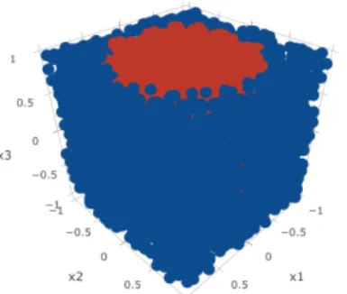
uniformly distributed on the interval [−1,1], so the data points form a cube. Class 1 is a cylinder in the middle of the cube whose section is a circle defined by the first two variables. The remainder forms class 2. The radius of the cylinder is chosen such that both classes have equal prior probability 0.5. An example of the resulting dataset is shown in Figure 2.
Fig. 1. Example of the dataset used for the experiment. The classes form a cylinder
(red points) in a cube (blue points). .
In summary, it is a binary classification task with two features (x1 and x2) which determine the
class and a meaningless one (x3) that does not have any influence in the actual class label of data
points.
2. Methodology
We created two independent sets: a training set of 1,000 observations (see Figure 2) and a test set of 500 observations. Models are trained on the training set of 1,000 examples. 5-fold cross validation is used for parameter tuning and model selection, except for the random forest model, for which the out-of-bag error is used instead. The test set is used to both compute the accuracy of the trained models and choose observations that are representative of the problem to be explained with the three explanation methods described in Part 1.
28 5. CYLINDER IN A CUBE
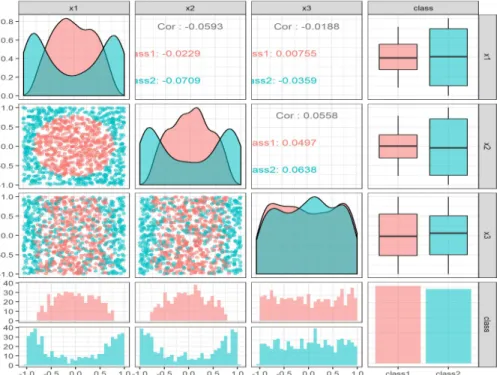
Fig. 2. Pairs plot of the training set. Each element of the matrix of plots displays the relationship between two variables in the dataset.
.
For LIME explanations, we produced linear explanations using K= 3, that is, using all features. In this case, since explanations composed of three parts are understandable for humans, there is no need to reduce the number of features used in the explanations1. Furthermore, we used asinterpretable representationthe resulting from converting the three continuous variables into three binary variables that specify whether an observation belongs to the same quantile (defined according to the training data) of the instance being explained or not. Since we want to explain each instance separately, the kernel width σ and the number of bins used to convert the original variables into binary are optimized separately for each observation based on the coefficient of determinationR2 of the linear
model obtained as explanation, which is a measure of the quality of the explanation. Although this is not a suggestion by the Ribeiro et al. , we think that this way we use the “best” hyperparameters to explain each obervation instead of a fixed set of hyperparameters for all instances which could not be useful for specific instances and lead to wrong explanations. Finally, we usedN= 10,000 samples.
For explanation vectors, there is only a hyperparameter σif we want to explain a hard classifier and we have to estimate the explanation vectors using a kernel density estimator. In that case, we optimized the value of the kernel widthσusing the test data as described in Chapter 3.
For IME, we used the sampling algorithm described in Chapter 4 (Section 3) withN = 10,000.
3. Explaining predictions
In this section, we will explain four predictions made by an artifficial neural network from the perspective of class 1 and using the three explanation methods: LIME (see Chapter 2), explanation
1However, in high dimensional problems we should choose a small number of featuresKin order to have an
understand-able explanation. The number of features could be optimized using the coefficient of correlationR2of the explanation
3. EXPLAINING PREDICTIONS 29
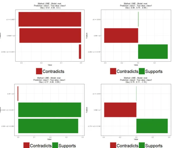
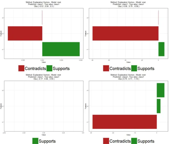
vectors (see Chapter 3) and IME (see Chapter 4). In order to facilitate the explanation process, we will visualize the explanations produced by any of the three methods with an horizontal bar chart that represents the contribution to the prediction of each considered variable, a common approach found in the literature (see References [1] or [7]). In addition, bars are green for features whose values influence the model in favor of the class being explained, and red for feature whose values influence the model against the class being explained. An example of this visualization is Figure 4.
The final neural network after tuning the hyperparameters has a single hidden layer with 5 neurons and decay parameterλ= 10−5. The accuracy of this model is 98.8% on the test data.
The instances that we will explain are four representative points of the problem from the test set: (1) Observation 1: a point close to the border of the cylinder with|x1| ≈ |x2|, ˜x(1)= (−0.53,0.56,0.3)
(2) Observation 2: a point close to the border of the cylinder withx1≈0, ˜x(2)= (−0.06,0.79,−0.96)
(3) Observation 3: a point close to the axis of the cylinder, ˜x(3) = (−0.17,0.06,0.99)
(4) Observation 4: a point close to the border of the cylinder withx2≈0, ˜x(4)= (0.79,0.11,−1.19)
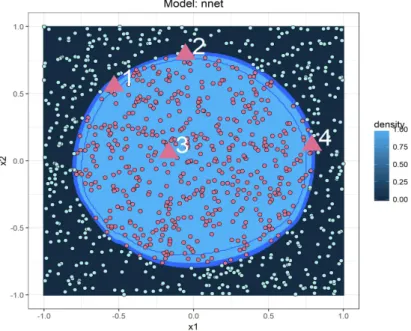
The first two variables (the meaningful ones) of these observations can be seen in Figure 3 along with the contour map of the probability functionf learned by the neural network when x3= 0. All
these observations are of actual class 1. The neural network is able to correctly classify observations 1 to 3, but it incorrectly predicts class 2 for observation 4. Specifically, the predicted probabilities (from the perspective of class 1) are: 0.9999820, 0.6556746, 1.0 and 0.1322022.
Fig. 3. Scatterplot of x2 against x1 of the training data (circular points) overlaid
on the contour map of the probability function f learned by a neural network when
x3= 0. Points inside the circle belong to class 1 (in violet) while points outside the
circle belong to class 2 (in turquoise). Also, four test points (triangular points) are displayed.
Theoretically, if the model were perfect, we would expect that the contribution of x3 to any
prediction was 0, while the contributions ofx1 andx2 should be different depending on their values.
First, it is reasonable to think that the prediction for observation 1 should take into account both
x1 andx2 in order to make a correct prediction because the combination of the two makes it more
30 5. CYLINDER IN A CUBE
observation 2 is extreme for a point of actual class 1, but the value ofx1makes it possible. Therefore,
the correct explanation for this prediction is that both features are important but in different ways: while the value ofx1 supports that the class is 1, the value of x2 contradicts this possibility. Third,
observation 3 is clearly from class 1 (because it is inside the cylinder) and bothx1andx2have typical
values of class 1, so both contribute to be class 1. Finally, observation 4 is comparable to observation 2 but with the opposite roles of variables 1 and 2, so the explanation for its prediction is that, despite the fact thatx1gives arguments against class 1, the actual class is 1 thanks tox2.
In the remaining part of this section we will discuss the explanations produced by the studied ex-planation methods and check if they are similar to the theoretical ones described in the last paragraph. The latter would be a first step to determine if the trained neural network has correctly learned when a data point belongs to class 1. However, in order to know for certain that we cantrustthis model, we would need to check explanations for much more predictions made by the model. At this point, it should be remembered that the explanations that we will obtain are specific for this neural network model and they could be completely different if we had used a different model because the learned probability functionf would be different.
3.1. LIME. The explanations produced by LIME are shown in Figure 4. First, we see that the method produces different explanations for different predictions, that is, it is able to determine that the model had different reasons behind each prediction. Second, we see that the explanations are in a binaryinterpretable representation, so this method has the advantage that it highlights the range of values of each feature that really has influence on the model’s prediction. For instance, stating that “the fact thatx1 has a value smaller than−0.4927 gives arguments against predicting class 1”
is more informative than just stating that “the value ofx1 gives arguments against predicting class
1”. Finally, it is worth noting that LIME would be able to produce simple (and short) explanations even in high dimensional problems because we can decide the number of variablesK to use for the explanations. Although the simple 3-dimensional data set that we are using in this chapter allows us to keep all three variables (i.e.,K= 3), this could make a big difference if our data set had hundreds or thousands of variables. However, the flexibility of LIME has the drawback that there are several hyperparameters that need to be set: the number of featuresKto use for each explanation, the kernel widthσthat determines the weight function to define the locality around the instance being explained and, in our case of tabular data, the number of groups used in the interpretable representation defined by converting continuous features into binary variables.
The best explanation found for observation 1 has σ = 1 and the continuous features are split into 4 groups. The coefficient of correlation of the interpretable linear model obtained, which can be interpreted as a measure of the explanation’s quality, isR2 = 0.19. The interpretable linear model
obtained is:
gx˜(1)(x) = ˆfx˜(1)(x) = 0.663−0.3141x1≤−0.4927(x)−0.311x2>0.49097(x)−0.011 10.0108<x3≤0.5371(x)
That is, the contributions of the features are: -0.314 forx1, -0.31 forx2and -0.011 forx3. According
to LIME, since the absolute value of the latter is very small compared to the other two, we can conclude that the model’s decision of predicting class 1 is influenced by bothx1 and x2, but not by
x3. Specifically, both meaningful features have the same influence on the prediction because they
have very similar absolute values and the sign of their contributions is negative, which means that their values reduce the probability of predicting class 1. This is reasonable because observation 1 is a data point with values ofx1 andx2 quite large for an observation that belongs to class 1. It may
seem counterintuitive that both meaningful variables gives arguments against predicting class 1 but the final prediction of the neural network is still class 1. This happens because the model intercept is larger than 0.5, which means that instances close to the observation (recall that LIME weights by the distance from the observation being explained) but that do not belong to any of the quartiles of the observation (recall that the explanation model is fitted using a binary interpretable representation) are more likely to belong to class 1. Therefore, the explanation for this prediction would be that
3. EXPLAINING PREDICTIONS 31
Fig. 4. LIME explanations for the predictions produced by a neural network for four
observations: ˜x(1)= (−0.53,0.56,0.3) (upper left), ˜x(2)= (−0.06,0.79,−0.96) (upper
right), ˜x(3)= (−0.17,0.06,0.99) (bottom left) and ˜x(4)= (0.79,0.11,−1.19) (bottom right).
the neural network (correctly) predicts class 1 for this observation because the given evidence against predicting this class by the fact that ˜x(1)1 ≤ −0.4927 and ˜x(1)2 > 0.49097 is not strong enough to change the predicted class of similar instances. This explanation coincides with the knowledge that we have of this data set and that we discussed in the previous section, which is an indication that the model has correctly learned the underlying function that determines the relationship between the three variables and the class.
The best explanation found for observation 2 has σ= 1 and the features are split into 5 groups. The coefficient of correlation of the interpretable linear model obtained isR2= 0.25. The interpretable
linear model obtained is:
gx˜(2)(x) = ˆfx˜(2)(x) = 0.52 + 0.358 1−0.208<x1≤0.187(x)−0.411x2>0.595(x) + 0.0041x3≤−0.616(x)
Again, the model’s decision of predicting class 1 is influenced by bothx1and x2, but in different
ways and being the role of x2 a little more important than the one of x1. On the one hand, the
value ofx1 supports that the class is 1 because its contribution has positive sign, which means that
having the value on the interval (−0.208,0.187) increases the probability of predicting class 1. On the other hand, the value ofx2 gives arguments against predicting t