What Energy Functions Can Be Minimized
via Graph Cuts?
Vladimir Kolmogorov,
Member,
IEEE, and Ramin Zabih,
Member,
IEEE
Abstract—In the last few years, several new algorithms based on graph cuts have been developed to solve energy minimization problems in computer vision. Each of these techniques constructs a graph such that the minimum cut on the graph also minimizes the energy. Yet, because these graph constructions are complex and highly specific to a particular energy function, graph cuts have seen limited application to date. In this paper, we give a characterization of the energy functions that can be minimized by graph cuts. Our results are restricted to functions of binary variables. However, our work generalizes many previous constructions and is easily applicable to vision problems that involve large numbers of labels, such as stereo, motion, image restoration, and scene reconstruction. We give a precise characterization of what energy functions can be minimized using graph cuts, among the energy functions that can be written as a sum of terms containing three or fewer binary variables. We also provide a general-purpose construction to minimize such an energy function. Finally, we give a necessary condition for any energy function of binary variables to be minimized by graph cuts. Researchers who are considering the use of graph cuts to optimize a particular energy function can use our results to determine if this is possible and then follow our construction to create the appropriate graph. A software implementation is freely available.
Index Terms—Energy minimization, optimization, graph algorithms, minimum cut, maximum flow, Markov Random Fields.
æ
1
I
NTRODUCTION ANDO
VERVIEWM
ANYof the problems that arise in early vision can be naturally expressed in terms of energy minimization. The computational task of minimizing the energy is usually quite difficult as it generally requires minimizing a nonconvex function in a space with thousands of dimen-sions. If the functions have a very restricted form, they can be solved efficiently using dynamic programming [2]. However, researchers typically have needed to rely on general purpose optimization techniques such as simulated annealing [3], [16], which requires exponential time in theory and is extremely slow in practice.In the last few years, however, a new approach has been developed based on graph cuts. The basic technique is to construct a specialized graph for the energy function to be minimized such that the minimum cut on the graph also minimizes the energy (either globally or locally). The minimum cut, in turn, can be computed very efficiently by max flow algorithms. These methods have been successfully used for a wide variety of vision problems, including image restoration [9], [10], [18], [21], stereo and motion [4], [9], [10], [20], [24], [27], [32], [35], [36], image synthesis [29], image segmentation [8], voxel occupancy [39], multicamera scene reconstruction [28], and medical imaging [5], [6], [25], [26]. The output of these algorithms is generally a solution with some interesting theoretical quality guarantee. In some cases [9], [18], [20], [21], [35], it is the global minimum, in other cases, a local minimum in a strong sense [10] that is within a known factor of the global
minimum. The experimental results produced by these algorithms are also quite good. For example, two recent evaluations of stereo algorithms using real imagery with dense ground truth [37], [41] found that the best overall performance was due to algorithms based on graph cuts.
Minimizing an energy function via graph cuts, however, remains a technically difficult problem. Each paper con-structs its own graph specifically for its individual energy function and, in some of these cases (especially [10], [27], [28]), the construction is fairly complex. One consequence is that researchers sometimes use heuristic methods for optimiza-tion, even in situations where the exact global minimum can be computed via graph cuts. The goal of this paper is to precisely characterize the class of energy functions that can be minimized via graph cuts and to give a general-purpose graph construction that minimizes any energy function in this class. Our results play a key role in [28], provide a significant generalization of the energy minimization methods used in [4], [5], [6], [10], [18], [26], [32], [39], and show how to minimize an interesting new class of energy functions.
In this paper, we only consider energy functions involving binary-valued variables. At first glance, this restriction seems severe since most work with graph cuts considers energy functions with variables that have many possible values. For example, the algorithms presented in [10] use graph cuts to address the standard pixel labeling problem that arises in early vision, including stereo, motion, and image restoration. In the pixel-labeling problem, the variables represent individual pixels and the possible values for an individual variable represent, e.g., its possible displacements or intensities. However, as we discuss in Section 2, many of the graph cut methods that handle multiple possible values work by repeatedly minimizing an energy function involving only binary variables. As we will see, our results generalize many graph cut algorithms [4], [5], [6], [10], [18], [26], [39] and can be easily applied to . The authors are with the Computer Science Department, Cornell
University, Ithaca, NY 14853. E-mail: {vnk, rdz}@cs.cornell.edu. Manuscript received 2 May 2002; revised 17 Mar. 2003; accepted 16 June 2003.
Recommended for acceptance by M.A.T. Figueiredo, E.R. Hancock, M. Pelillo, and J. Zerubia.
For information on obtaining reprints of this article, please send e-mail to: [email protected], and reference IEEECS Log Number 118731.
problems like pixel labeling, even though the pixels have many possible labels.
1.1 Summary of Our Results
In this paper, we focus on two classes of energy functions. Let fx1;. . .; xng,xi 2 f0;1gbe a set of binary-valued variables.
We define the classF2to be functions that can be written as a
sum of functions of up to two binary variables at a time,
Eðx1;. . .; xnÞ ¼ X i EiðxiÞ þ X i<j Ei;jðxi; xjÞ: ð1Þ
We define the classF3to be functions that can be written as
a sum of functions of up to three binary variables at a time,
Eðx1;. . .; xnÞ ¼ X i EiðxiÞ þ X i<j Ei;jðxi; xjÞ þ X i<j<k Ei;j;kðxi; xj; xkÞ: ð2Þ
Obviously, the class F2 is a strict subset of the class F3.
However, to simplify the discussion, we will begin by focusing onF2. Note that there is no restriction on the signs
of the energy functions or of the individual terms. The main results in this paper are:
. A precise characterization of the class of functions in F3that can be minimized using graph cuts.
. A general-purpose graph construction for minimiz-ing any function in this class.
. A necessary condition for any function of binary variables to be minimized via graph cuts.
The rest of the paper is organized as follows: In Section 2, we describe how graph cuts can be used to minimize energy functions and discuss the importance of energy functions with binary variables in the context of two example vision problems, namely, stereo and multicamera scene reconstruc-tion. In Section 3, we formalize the relationship between graphs and energy functions and provide a precise definition of the problem that we wish to solve. Section 4 contains our main theorem for the class of functionsF2and shows how this
result can be used for both stereo and multicamera scene reconstruction. Section 5 gives our results for the broader class F3
and shows how this result can be used for multicamera scene reconstruction. A necessary condition for an arbitrary function of binary variables to be minimized via graph cuts is presented in Section 6. We discuss some related work in the theory of submodular functions in Section 7 and give a summary of our graph constructions in Section 8. Software can be downloaded from http://www.cs.cornell.edu/~rdz/ graphcuts.html that automatically constructs the appropriate graph and minimizes the energy. An NP-hardness result and a proof of one of our theorems are deferred to the Appendix.
2
M
INIMIZINGE
NERGYF
UNCTIONS VIAG
RAPHC
UTSMany vision problems, especially in early vision, can naturally be formulated in terms of energy minimization. Energy minimization has a long history in computer vision (see [34] for several examples). The classical use of energy minimization is to solve the pixel-labeling problem, which is a generalization of such problems as stereo, motion, and image restoration. The input is a set of pixelsPand a set of
labels L. The goal is to find a labeling f (i.e., a mapping fromPtoL) which minimizes some energy function.
A standard form of the energy function is
EðfÞ ¼X p2P DpðfpÞ þ X p;q2N Vp;qðfp; fqÞ; ð3Þ
where N P P is a neighborhood system on pixels.1
DpðfpÞ is a function derived from the observed data that
measures the cost of assigning the label fp to the pixel p.
Vp;qðfp; fqÞmeasures the cost of assigning the labelsfp; fqto
the adjacent pixels p; q and is used to impose spatial smoothness. At the borders of objects, adjacent pixels should often have very different labels and it is important thatEnot overpenalize such labelings. This requires that V be a nonconvex function ofjfpfqj. Such an energy function is
calleddiscontinuity-preserving. Energy functions of the form (3) can be justified on Bayesian grounds using the well-known Markov Random Fields (MRF) formulation [16], [31]. Energy functions like E are extremely difficult to minimize, however, as they are nonconvex functions in a space with many thousands of dimensions. They have traditionally been minimized with general-purpose optimi-zation techniques (such as simulated annealing) that can minimize an arbitrary energy function. As a consequence of their generality, however, such techniques require expo-nential time and are extremely slow in practice. In the last few years, however, efficient algorithms have been devel-oped for these problems based on graph cuts.2
2.1 Graph Cuts
Suppose G ¼ ðV;EÞ is a directed graph with nonnegative edge weights that has two special vertices (terminals), namely, the sourcesand the sinkt. Ans-t-cut (which we will refer to informally as a cut)C¼S; Tis a partition of the vertices inVinto two disjoint sets SandT such thats2S
andt2T. The cost of the cut is the sum of costs of all edges that go fromStoT:
cðS; TÞ ¼ X
u2S;v2T ;ðu;vÞ2E
cðu; vÞ:
The minimums-t-cut problem is to find a cutCwith the smallest cost. Due to the theorem of Ford and Fulkerson [14], this is equivalent to computing the maximum flow from the source to sink. There are many algorithms that solve this problem in polynomial time with small constants [1], [7], [17]. It is convenient to note a cut C¼S; T by a labeling f
mapping from the set of the vertices V fs; tg to f0;1g, where fðvÞ ¼0 means that v2S and fðvÞ ¼1 means that
v2T. We will use this notation later.
Note that a cut is abinarypartition of a graph viewed as a labeling; it is a binary-valued labeling. While there are generalizations of the minimum s-t-cut problem that involve more than two terminals (such as the multiway cut problem [12]), such generalizations are NP-hard.
1. Without loss of generality, we can assume that N contains only ordered pairsp; qfor whichp < qsince we can combine two termsVp;qand
Vq;pinto one term.
2. It is interesting to note that some similar techniques have been developed by algorithms researchers working on the task assignment problem [30], [33], [40].
2.2 Energy Minimization Using Graph Cuts
In order to minimizeEusing graph cuts, a specialized graph is created such that the minimum cut on the graph also minimizesE(either globally or locally). The form of the graph depends on the exact form ofV and on the number of labels. In certain restricted situations, it is possible to efficiently compute the global minimum. If there are only two labels, [18] showed how to compute the global minimum ofE. This is also possible for an arbitrary number of labels as long as the labels are consecutive integers andV is theL1distance. The
construction is due to [20] and is a modified version of [36]. This construction has been further generalized to handle an arbitrary convexV [22].
However, a convexV is not discontinuity preserving and optimizing an energy function with such a V leads to oversmoothing at the borders of objects. The ability to find the global minimum efficiently, while theoretically of great value, does not overcome this drawback. This is clearly visible in the relatively poor performance of such algo-rithms on the stereo benchmarks described in [37].
Moreover, efficient global energy minimization algo-rithms for even the simplest class of discontinuity-preserving energy functions almost certainly do not exist. Consider
Vðfp; fqÞ ¼T½fp6¼fq, where the indicator functionT½is 1 if
its argument is true and otherwise 0. This smoothness term, sometimes called the Potts model, is clearly discontinuity-preserving. Yet, it is known to be NP-hard to minimize [10].
However, graph cut algorithms have been developed that compute a local minimum in a strong sense [10]. As we shall see, these methods minimize an energy function with nonbinary variables by repeatedly minimizing an energy function with binary variables.3
2.3 The Expansion Move Algorithm
One of the most effective algorithms for minimizing discontinuity-preserving energy functions is the expansion move algorithm, which was introduced in [10]. This algorithm can be used wheneverV is a metric on the space of labels; this includes several important discontinuity-preserving energy functions (see [10] for more details).
Consider a labeling f and a particular label . Another labeling f0is defined to be an-expansion move fromf if
fp0 6¼ implies fp0 ¼fp. This means that the set of pixels
assigned the label has increased when going from f to
f0. An example of an expansion move is shown in Fig. 1. The expansion move algorithm cycles through the labels
in some order (fixed or random) and finds the lowest energy
-expansionmove from the current labeling. If this expansion move has lower energy than the current labeling, then it becomes the current labeling. The algorithm terminates with a labeling that is a local minimum of the energy with respect to expansion moves; more precisely, there is no -expansion
move, for any label, with lower energy. It is also possible to prove that such a local minimum lies within a multiplicative factor of the global minimum [10] (the factor is at least 2 and depends only onV).
2.3.1 Applications of the Expansion Move Algorithm
Energy functions like that of (3) arise commonly in early vision, so it is straightforward to apply the expansion move algorithm to many vision problems. For example, the expansion move algorithm can be used for the standard 2-camera stereo problem, as well as for multicamera scene reconstruction.
Stereo. For the stereo problem, the labels are disparities and the data term DpðfpÞ is some function of the intensity
difference between the pixelpin the primary image and the pixelpþfpin the secondary image. On the stereo problem, the
expansion move algorithm and other closely related energy minimization algorithms give very strong empirical perfor-mance. They have been used as a critical component of several algorithms [4], [27], [28], [32], including the top two algo-rithms (and five of the top six) according to a recent published survey [37] that used real data with dense ground truth.
Multicamera scene reconstruction. It is also possible to use the expansion move algorithm for multicamera scene reconstruction, as reported in [28]. In their problem formula-tion, the energy function consists entirely of terms with two arguments (in other words, Dp does not exist). The set of
pixelsPincludes all pixels from all cameras and the labels correspond to planes. Thus, a pairhp; fpispecifies a 3D point
and a labelingfgives the nearest scene element visible in each pixel in each camera.
The expansion move algorithm can be straightforwardly applied to this problem as long as the energy is of the right form. Note that an -expansion move increases the set of pixels labeled in all cameras at once, rather than in a single preferred image.
The actual energy function consists of three terms. All the terms are in the same form asVin that they depend on pairs of labelsfp; fq. One term enforces the visibility constraint. While
this constraint is very important, it has no analogue in the simple pixel labeling problem formulation and we will not discuss it here. The other terms are analogous to the standard stereo data term and smoothness term.
In the multicamera scene reconstruction problem, the data term enforces photoconsistency. LetI be a set of pairs of “nearby” 3D points. These points will come from different cameras, but they will share the same depth (i.e., the points are of the formhp; fpi;hq; fqiwherefp¼fqandp; qare pixels
from different cameras). Then, the data term is
X
fhðp;lÞi;hðq;lÞi2Ig
Dp;q;lðfp; fqÞ; ð4Þ
where
Dp;q;lðfp; fqÞ ¼Dðp; qÞ T½fp¼fq¼l:
We have rewritten each term in the sum as a function of
fp; fq(sincep; qdo not depend onf). The functionDwill be
3. This is somewhat analogous to theZMalgorithm [13], although that method produces a global minimum of a function with nonbinary variables by repeatedly minimizing a function with binary variables.
Fig. 1. An example of an expansion move. The labeling on the right is a white-expansion move from the labeling on the left.
some function of the intensity difference betweenp andq, typically, a monotonically increasing function.
The smoothness term, on the other hand, involves a single camera at a time. It is defined to be
X
fp;qg2N
Vp;qðfp; fqÞ; ð5Þ
where N is a neighborhood system on pixels in a single camera.
2.4 Energy Functions of Binary Variables
The key subproblem in the expansion move algorithm is to compute the lowest energy labeling within a single
-expansionoff. This subproblem is solved efficiently with a single graph cut [10], using a somewhat intricate graph construction.
It is important to note that this subproblem is an energy minimization problem over binary variables, even though the overall problem that the expansion move algorithm is solving involves nonbinary variables. This is because each pixel will either keep its old value underfor acquire the new label.
Formally, any labeling f0within a single-expansion of the initial labeling f can be encoded by a binary vector
x¼ fxpjp2 Pg, where f0ðpÞ ¼fðpÞ if xp¼0 and f0ðpÞ ¼
if xp¼1. Let us denote the labeling defined by a binary
vectorxasfx. Since the energy functionE is defined over
all labelings, it is obviously also defined over labelings specified by binary vectors. The key step in the expansion move algorithm is therefore to find the minimum ofEðfxÞ
over all binary vectors x.
The importance of energy functions of binary variables does not arise simply from the expansion move algorithm. Instead, it results from the fact that a graph cut effectively assigns one of two possible values to each vertex of the graph. So, in a certain sense, any energy minimization construction based on graph cuts relies on intermediate binary variables.
It is, of course, possible to use graph cuts in such a manner that variables in the original problem do not correspond in a one-to-one manner with vertices in the graph. This kind of complex transformation lies at the heart of the graph cut algorithms that compute a global minimum [20], [22]. However, the NP-hardness result given in [10] shows that (unless P = NP) such result cannot be achieved for even the simplest discontinuity-preserving energy function.
3
R
EPRESENTINGE
NERGYF
UNCTIONS WITHG
RAPHSLet us consider a graphG ¼ ðV;EÞwith terminalssandt, thus V ¼ fv1;. . .; vn; s; tg. Each cut onGhas some cost; therefore,G
represents the energy function mapping from all cuts onGto the set of nonnegative real numbers. Any cut can be described bynbinary variablesx1;. . .; xncorresponding to vertices inG
(excluding the source and the sink):xi¼0whenvi2Sand
xi¼1whenvi2T. Therefore, the energyEthatGrepresents
can be viewed as a function ofnbinary variables:Eðx1;. . .; xnÞ
is equal to the cost of the cut defined by the configuration
x1;. . .; xn (xi2 f0;1g). Note that the configuration that
minimizesEwill not change if we add a constant toE. We can efficiently minimizeEby computing the minimum
s-t-cut onG. This naturally leads to the question: What is the class of energy functionsEfor which we can construct a graph
that representsE? We can also generalize our construction. Above, we used each vertex (except the source and the sink) for encoding one binary variable. Instead, we can specify a subsetV0¼ fv1;. . .; vkg V fs; tgand introduce variables
only for the vertices in this set. Then, there may be several cuts corresponding to a configurationx1;. . .; xk. If we define the
energyEðx1;. . .; xkÞas the minimum among the costs of all
such cuts, then the minimums-t-cut onGwill again yield the configuration which minimizesE.
We will summarize the graph constructions that we allow in the following definition.
Definition 3.1.A functionEofnbinary variables is called graph-representableif there exists a graphG ¼ ðV;EÞwith terminals
sandtand a subset of verticesV0¼ fv1;. . .; vng V fs; tg
such that, for any configurationx1;. . .; xn, the value of the
energyEðx1;. . .; xnÞis equal to a constant plus the cost of the
minimums-t-cut among all cutsC¼S; T in whichvi2S, if
xi¼0, and vi2T, if xi¼1(1in). We say thatE is
exactly representedbyG,V0if this constant is zero.
The following lemma is an obvious consequence of this definition.
Lemma 3.2.Suppose the energy functionEis graph-representable
by a graphGand a subsetV0. Then, it is possible to find the exact
minimum ofEin polynomial time by computing the minimum
s-t-cut onG.
In this paper, we will give a complete characterization of the classesF2andF3in terms of graph representability and
show how to construct graphs for minimizing graph-representable energies within these classes. Moreover, we will give a necessary condition for all other classes that must be met for a function to be graph-representable. Obviously, it would be sufficient to consider only the class F3 since
F2 F3
. However, the condition forF2
is simpler, so we will consider it separately.
Note that the energy functions we consider can be negative, as can the individual terms in the energy functions. However, the graphs that we construct must have nonnega-tive edge weights. All previous work that used graph cuts for energy minimization dealt with nonnegative energy func-tions and terms.
4
T
HEC
LASSF
2Our main result for the classF2is the following theorem. Theorem 4.1 (F2 Theorem).Let E be a function of n binary
variables from the classF2
, i.e., Eðx1;. . .; xnÞ ¼ X i EiðxiÞ þ X i<j Ei;jðxi; xjÞ: ð6Þ
Then,E is graph-representable if and only if each term Ei;j
satisfies the inequality
Ei;jð0;0Þ þEi;jð1;1Þ Ei;jð0;1Þ þEi;jð1;0Þ: ð7Þ
We will call functions satisfying the condition of (7)
regular.4 This theorem thus states that regularity is a
necessary and sufficient condition for graph-representabil-ity, at least inF2.
4. The representation of a functionE as a sum in (6) is not unique. However, we will show in Section 5 that the definition of regularity does not depend on this representation.
In this section, we will give a constructive proof that regularity is a sufficient condition by describing how to build a graph that represents an arbitrary regular function inF2
. The other half of the theorem is proven in much more generality in Section 6, where we show that a regularity is a necessary condition for any function to be graph-representable.
Regularity is thus an extremely important property as it allows energy functions to be minimized using graph cuts. Moreover, without the regularity constraint, the problem becomes intractable. Our next theorem shows that mini-mizing an arbitrary nonregular function is NP-hard, even if we restrict our attention toF2.
Theorem 4.2 (NP-Hardness).LetE2be a nonregular function
of two variables. Then, minimizing functions of the form Eðx1;. . .; xnÞ ¼ X i EiðxiÞ þ X ði;jÞ2N E2ðxi; xjÞ;
where Ei are arbitrary functions of one variable and
N fði; jÞj1i < jng, is NP-hard.
The proof of this theorem is deferred to the Appendix. Note that this theorem implies the intractability of mini-mizing the entire class of nonregular functions inF2
. It thus allows for the existence of nonregular functions in F2that
can be minimized efficiently.5 4.1 Graph Construction forF2
In this section, we will prove the constructive part of the F2theorem. LetEbe a regular function of the form given in
the theorem. We will construct a graph for each term separately and then “merge” all graphs together. This is justified by the additivity theorem, which is given in the Appendix.
The graph will containnþ2vertices:V ¼ fs; t; v1;. . .; vng.
Each nonterminal vertexviwill encode the binary variablexi.
For each term ofE, we will add one or more edges that we describe next.
First, consider a termEidepending on one variablex i. If
Eið0Þ< Eið1Þ, then we add the edgeðs; v
iÞwith the weight
Eið1Þ Eið0Þ(Fig. 2a). Otherwise, we add the edgeðv
i; tÞwith
the weightEið0Þ Eið1Þ(Fig. 2b). It easy to see that, in both
cases, the constructed graph represents the functionEi(but
with different constants:Eið0Þin the former case andEið1Þin the latter).
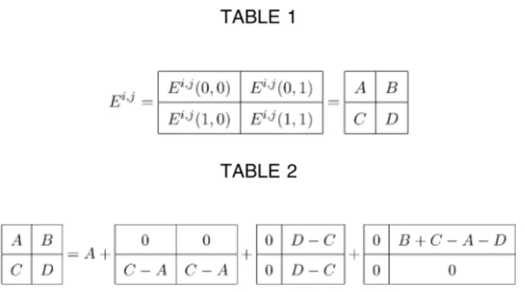
Now, consider a termEi;jdepending on two variablesxi,
xj. It is convenient to represent it in Table 1. We can rewrite
it as it is expressed in Table 2. The first term is a constant function, so we don’t need to add any edges for it. The second and the third terms depend only on one variablexi
andxj, respectively. Therefore, we can use the construction
given above. To represent the last term, we add an edge ðvi; vjÞ with the weight BþCAD (Fig. 2c). Note that
this weight is nonnegative due to the regularity ofE. A complete graph forEi;j will contain three edges. One possible case (CA >0 and DC <0) is illustrated in Fig. 2d.
Note that we did not introduce any additional vertices for representing binary interactions of binary variables. This is in contrast to the construction in [10] which added auxiliary vertices for representing energies that we just considered. Our construction yields a smaller graph and, thus, the minimum cut can potentially be computed faster. 4.2 Example: Applying Our Results for Stereo and
Multicamera Scene Reconstruction
Our results give a generalization of a number of previous algorithms [4], [5], [6], [10], [18], [26], [32], [39] in the following sense. Each of these methods used a graph cut algorithm that was specifically constructed to minimize a certain form of energy function. The class of energy functions that we show how to minimize is much larger and includes the techniques used in all of these methods as special cases.
To illustrate the power of our results, we return to the use of the expansion move algorithm for stereo and multicamera scene reconstruction described in Section 2.3.1. Recall that the key subproblem is to find the minimum energy labeling within a single -expansion of f, which is equivalent to minimizing the energy over binary variablesxi.
Fig. 2. Graphs that represent some functions inF2. (a) Graph forEi,
whereEið0Þ> Eið1Þ. (b) Graph forEi, whereEið0Þ 6> Eið0Þ. (c) Third
edge forEi;j. (d) Complete graph forEi;jifC > AandC > D.
5. Gortler et al. have investigated a particularly simple example, namely, functions that can be made regular by interchanging the senses of 0 and 1 for some set of variables.
TABLE 1
4.2.1 Stereo
The paper that proposed the expansion move algorithm [10] showed how to solve the key subproblem with graph cuts as long asDpis nonnegative andV is a metric on the space
of labels. This involved an elaborate graph construction and several associated theorems.
Using our results, we can recreate the proof that such an energy function can be solved in just a few lines. All that we need is to prove thatEis regular ifDpis nonnegative andV
is a metric. Obviously, the form of Dp doesn’t matter; we
simply have to show that if V is a metric the individual terms satisfy the inequality in (7). Table 3 considers two neighboring pixelsp; q, with associated binary variablesi; j. IfV is a metric, by definition, for any labels; ; Vð; Þ ¼
0andVð; Þ þVð; Þ Vð; Þ. This gives the inequality of (7) and shows thatEcan be minimized using graph cuts.
4.2.2 Multicamera Scene Reconstruction
We can also show that the expansion move algorithm can be used for a different energy function, namely, the one proposed for multicamera scene reconstruction in [28]. We need to show that the smoothness (5) and the data (4) energy functions are regular. The argument for the smoothness term is identical to the one we just gave for stereo because the smoothness term is regular.
The data term for multicamera scene reconstruction is perhaps the best demonstration of the utility of our results. The function in the data term is clearly not a metric on the space of labels (for example, it is entirely possible that
Dp;q;lð; Þ 6¼0for some label). Prior to our results, the only
way to use the expansion move algorithm for this energy function would be to create an elaborate graph construction that is specific to this particular energy function. Worse, it was not a priori obvious that such a construction existed.
Using our results, it is simple to show that the data term can be made regular and the expansion move algorithm can be applied. Let us write out the sum in (4) and consider a single termDðp; qÞ T½fp¼fq¼l, which imposes a penalty ifpandq
both have the labell. Recall that we are seeking the lowest energy labeling within a single-expansionoff. We will have two binary variables which are 0 if the associated pixel keeps its original label infand 1 if it acquires the new label.
There are two cases that must be analyzed separately:l6¼
andl¼. Consider the casel6¼. Iffp6¼lorfq 6¼l, then the
term is zero for any values of the binary variables. If
fp¼fq ¼l, then the penalty is only imposed when the binary
variables are both 0. We can graphically show this in Table 4.
Ifl¼, then, if eitherfporfqare, the penalty imposed is
independent of one of the binary variables and it is easy to see that this is regular. Ifl¼and neitherfpnorfqare, then the
penalty is only imposed when the binary variables are both 1. Graphically, this can be shown in Table 5. Overall, the energy function is regular ifDðp; qÞis nonpositive. Recall thatDðp; qÞ is a photoconsistency term. It is typically a monotonically increasing function of the intensity difference betweenpand
q. By simply subtracting a large constant, we can ensure thatD
is nonpositive and, thus, apply our construction.
5
T
HEC
LASSF
3Before stating our theorem for the classF3
, we will extend the definition of regularity to arbitrary functions of binary variables. This requires a notion ofprojections.
Suppose we have a functionE of n binary variables. If we fixmof these variables, then we get a new functionE0of
nmbinary variables; we will call this function aprojection
ofE. The notation for projections is as follows:
Definition 5.1. Let Eðx1;. . .; xnÞ be a function of n binary
variables and letI,Jbe a disjoint partition of the set of indices
f1;. . .; ng: I¼ fið1Þ;. . .; iðmÞg, J¼ fjð1Þ;. . .; jðnmÞg. Let ið1Þ;. . .; iðmÞ be binary constants. A projection E0¼
E½xið1Þ¼ið1Þ;. . .; xiðmÞ¼iðmÞ is a function of nm
variables defined by
E0ðxjð1Þ;. . .; xjðnmÞÞ ¼Eðx1;. . .; xnÞ;
where xi¼i for i2I. We say that we fix the variables
xið1Þ, . . ., xiðmÞ.
Now, we can give a generalized definition of regularity.
Definition 5.2.
. All functions of one variable are regular.
. A function E of two variables is called regular if
Eð0;0Þ þEð1;1Þ Eð0;1Þ þEð1;0Þ.
. A function E of more than two variables is called
regular if all projections of E of two variables are
regular.
For the classF2, this definition is equivalent to the previous
one. A proof of this fact is given in Section 5.3.
Now, we are ready to formulate our main theorem forF3. Theorem 5.3 (F3
Theorem).Let E be a function of n binary
variables fromF3, i.e.,
Eðx1;. . .; xnÞ ¼ X i EiðxiÞ þ X i<j Ei;jðxi; xjÞ þ X i<j<k Ei;j;kðxi; xj; xkÞ: ð8Þ
Then,E is graph-representable if and only ifEis regular.
TABLE 3
TABLE 4
5.1 Graph Construction forF3
Consider a regular functionEof the form given in (8). The regularity ofEdoes not necessarily imply that each term in (8) is regular. However, we will give an algorithm for converting any regular function inF3
to the form (8) where each term is regular (see the regrouping theorem in the next section). Note that this was not necessary for the class F2
since, for any representation of a regular function in the form (6), each term in the sum is regular.
Here, we will give graph construction for a regular functionEof the form as in theF3
theorem assuming that each term of E is regular. The graph will contain
nþ2 vertices: V ¼ fs; t; v1;. . .; vng as well as some
addi-tional vertices described below. Each nonterminal vertexvi
will encode the binary variable xi. For each term ofE, we
will add one or more edges and, possibly, an additional (unique) vertex that we describe next. Again, our construc-tion is justified by the additivity theorem given in the Appendix.
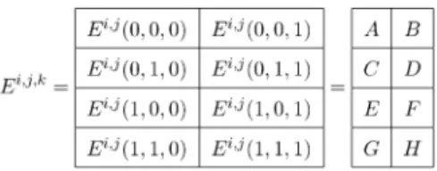
Terms depending on one and two variables were considered in the previous section, so we will concentrate on a term Ei;j;k depending on three variables x
i, xj, xk. It
is convenient to represent it in Table 6.
Let us denote P ¼ ðAþDþFþGÞ ðBþCþEþHÞ. We consider two cases:
Case 1.P >¼0.Ei;j;kcan be rewritten as shown in Table 7,
whereP1¼FB,P2¼GE,P3¼DC,P23¼BþC
AD,P31¼BþEAF,P12¼CþEAG.Ei;j;k is
regular, therefore, by considering projectionsEi;j;k½x1¼0,
Ei;j;k½x
2¼0,Ei;j;k½x3¼0, we conclude thatP23,P31,P12are
nonnegative.
The first term is a constant function, so we don’t need to add any edges for it. The next three terms depend only on one variable (xi,xj,xk, respectively), so we can use the
construc-tion given in the previous secconstruc-tion. The next three terms depend on two variables; the nonnegativity ofP23,P31,P12
implies that they are all regular. Therefore, we can again use the construction of the previous section. (Three edges will be added: ðvj; vkÞ, ðvk; viÞ, ðvi; vjÞ with weights P23, P31, P12,
respectively).
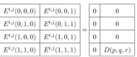
To represent the last term, we will add an auxiliary vertex
uijkand four edgesðvi; uijkÞ,ðvj; uijkÞ,ðvk; uijkÞ,ðuijk; tÞwith the
weightP. This is shown in Fig. 3a. Let us prove these four edges exactly represent the function shown in Table 8. If
xi¼xj¼xk¼1, then the cost of the minimum cut is0(the
minimum cut isS¼ fsg,T ¼ fvi; vj; vk; uijk; tg. Suppose at
least one of the variables xi, xj, xk is 0; without loss of
generality, we can assume thatxi¼0, i.e.,vi2 S. Ifuijk2S,
then the edgeðuijk; tÞis cut; ifuijk2T, the edgeðvi; uijkÞis cut
yielding the costP. Hence, the cost of the minimum cut is at leastP. However, ifuijk2S, the cost of the cut is exactlyP, no
matter where the verticesvi,vj,vkare. Therefore, the cost of the
minimum cut will be0ifxi¼xj¼xk¼1andPotherwise, as
desired.
Case 2.P <0. This case is similar to the Case 1.Ei;j;kcan
be rewritten as shown in Table 9, where P1¼CG,
P2¼BD, P3¼EF, P32¼FþGEH, P13¼Dþ
G CH, P21¼DþFBH. By considering
projec-tionsEi;j;k½x
1¼1, Ei;j;k½x2¼1, Ei;j;k½x3¼1, we conclude
thatP32,P13,P21are nonnegative.
As in the previous case, all terms except the last are regular and depend on at most two variables, so we can use the construction of the previous section. We will have, for example, edgesðvk; vjÞ,ðvi; vkÞ,ðvj; viÞwith weightsP32,P13,
P21, respectively.
To represent the last term, we will add an auxiliary vertex uijk and four edges ðuijk; viÞ, ðuijk; vjÞ, ðuijk; vkÞ,
ðs; uijkÞwith the weight P. This is shown in Fig. 3b.
TABLE 6
Fig. 3. Graphs for functions inF3. (a) Edge weights are allP. (b) Edge
weights are allP.
TABLE 7
Note that, in both cases, we added an auxiliary vertex
uijk. It is easy to see that this is necessary since graphs
without auxiliary vertices can only represent functions in F2
. Each edge represents a function of at most two variables, so the whole graph represents a function that is a sum of terms of at most two variables.
5.2 Constructive Proof of the Regrouping Theorem Now, we will show how to convert a regular function inF3
to the form given in (8) where each term is regular.
Theorem 5.4 (regrouping). Any regular function E from the
classF3can be rewritten as a sum of terms such that each term
is regular and depends on at most three variables.
We will assumeEgiven as
Eðx1;. . .; xnÞ ¼
X
i<j<k
Ei;j;kðxi; xj; xkÞ;
wherei,j,kare indices from the setf1;. . .; ng(we omitted terms involving functions of one and two variables since they can be viewed as functions of three variables).
We begin by giving a definition.
Definition 5.5.The functionalwill be a mapping from the set of all functions (of binary variables) to the set of real numbers
which is defined as follows. For a functionEðx1;. . .; xnÞ
ðEÞ ¼ X
x12f0;1g;...;xn2f0;1g
ni¼1ð1Þxi
Eðx1;. . .; xnÞ:
For example, for a function E of two variables ðEÞ ¼
Eð0;0Þ Eð0;1Þ Eð1;0Þ þEð1;1Þ. Note that a functionE
of two variables is regular if and only ifðEÞ 0. It is trivial to check the following lemma.
Lemma 5.6.The functionalhas the following properties.
. is linear, i.e., for a scalarc and two functions E0,
E00 of n variables ðE0þE00Þ ¼ðE0Þ þðE00Þ and
ðcE0Þ ¼cðE0Þ.
. IfEis a function ofnvariables that does not depend on
at least one of the variables, thenðEÞ ¼0.
We will prove the theorem using the following lemma and a trivial induction argument.
Definition 5.7. Let Ei;j;k be a function of three variables. The
functionalNðEi;j;kÞis defined as the number of projections of
two variables ofEi;j;kwith positive values of the functional.
Note thatNðEi;j;kÞ ¼0exactly whenEi;j;kis regular.
Lemma 5.8. Suppose the function E of n variables can be written as
Eðx1;. . .; xnÞ ¼
X
i<j<k
Ei;j;kðxi; xj; xkÞ;
where some of the terms are not regular. Then, it can be written as Eðx1;. . .; xnÞ ¼ X i<j<k ~ E Ei;j;kðxi; xj; xkÞ; where X i<j<k NEE~i;j;k< X i<j<k N E i;j;k:
Proof. For simplicity of notation, let us assume that the term E1;2;3 is not regular and ðE1;2;3½x
3¼0Þ>0 or
ðE1;2;3½x3¼1Þ>0 (we can ensure this by renaming
indices). Let Ck¼ max k2f0;1g ðE1;2;k½xk¼kÞ k2 f4;. . .; ng C3¼ Xn k¼4 Ck:
Now, we will modify the terms E1;2;3, . . ., E1;2;n as
follows:
~
E
E1;2;kE1;2;kR½Ck k2 f3;. . .; ng;
where R½C is the function of two variables x1 and x2
defined by Table 10 (other terms are unchanged:
~
E
Ei;j;kEi;j;k,ði; jÞ 6¼ ð1;2Þ). We have
Eðx1;. . .; xnÞ ¼ X i<j<k ~ E Ei;j;kðxi; xj; xkÞ sincePnk¼3Ck¼0andPnk¼3R½Ck 0.
If we considerR½Cas a function ofnvariables and take a projection of two variables where the two variables that are not fixed arexiandxj(i < j), then the functionalwill
beC, ifði; jÞ ¼ ð1;2Þ, and0otherwise (since, in the latter case, a projection actually depends on, at most, one variable). Hence, the only projections of two variables that could have changed their value of the functional are
~ E E1;2;k½x 3¼3;. . .; xn¼n,k2 f3;. . .; ng, if we treatEE~1;2;k as functions ofn variables, orEE~1;2;k½x k¼k, if we treat ~ E
E1;2;kas functions of three variables.
TABLE 9
First, let us consider terms with k2 f4;. . .; ng. We haveðE1;2;k½x k¼kÞ Ck, thus ðEE~1;2;k½x k¼kÞ ¼ðE1;2;k½xk¼kÞ ðR½Ck½xk¼kÞ CkCk¼0:
Therefore, we did not introduce any nonregular projec-tions for these terms.
Now, let us consider the term ðEE~1;2;3½x
3¼3Þ. We can write ðEE~1;2;3½x3¼3Þ ¼ðE1;2;3½x3¼3Þ ðR½C3½x3¼3Þ ¼ðE1;2;3½x3¼3Þ ð Xn k¼4 CkÞ ¼ Xn k¼3 ðE1;2;k½xk¼kÞ;
wherek¼arg max2f0;1gðE1;2;k½xk¼Þ,k2 f4;. . .; ng.
The last expression is justðE½x3¼3;. . .; xn¼nÞand
is nonpositive sinceE is regular by assumption. Hence, values ðEE~1;2;3½x
3¼0Þ and ðEE~1;2;3½x3¼1Þ are both
nonpositive and, therefore, the number of nonregular
projections has decreased. tu
The complexity of a single step isOðnÞsince it involves modifying at mostnterms. Therefore, the complexity of the whole algorithm isOðmnÞ, wheremis the number of terms in (8) since, in the beginning,Pi<j<kNðEi;j;kÞis at most6m
and each step decreases it by at least one. 5.3 The Two Definitions of Regularity
Are Equivalent
We now prove that the definition of regularity 5.2 is equivalent to the previous definition of regularity for the classF2
. Note that the latter one is formulated not only as a property of the function E but also as a property of its representation as a sum in (6). We will show equivalence for an arbitrary representation, which will imply that the definition of regularity for the classF2depends only onE
but not on the representation.
Let us consider a graph-representable function E from the classF2: Eðx1;. . .; xnÞ ¼ X i EiðxiÞ þ X i<j Ei;jðxi; xjÞ:
Consider a projection where the two variables that are not fixed are xi and xj. By Lemma 5.6, the value of the
functional of this projection is equal to ðEi;jÞ (all other
terms yield zero). Therefore, this projection is regular if and only if Ei;jð0;0Þ þEi;jð1;1Þ Ei;jð0;1Þ þEi;jð1;0Þ, which
means that the two definitions are equivalent.
5.4 Example: Multicamera Scene Reconstruction We now show an example of function from the classF3that
is potentially useful in vision. Consider the multicamera scene reconstruction problem described earlier. Similar to the data term depending on pairs of pixels, we can define a term depending on triples of pixels.6LetI3be a set of triples
of “nearby” 3D points. These points will come from three different cameras, but they will share the same depth (i.e., the points are of the form hp; fqi;hq; fqi;hr; fri, where fp¼
fq¼fr and p; q; r are pixels from different cameras). The
new data term will be
X
fhp;li;hq;li;hr;li2I3g
Dp;q;r;lðfp; fq; frÞ; ð9Þ
where
Dp;q;r;lðfp; fq; frÞ ¼Dðp; q; rÞ T½fp¼fq ¼fr¼l:
This term can be motivated as follows: If three pixels have similar intensities, then it is more likely that they see the same scene element than if only two pixels have similar intensities. We now show the expansion move algorithm can be used for minimizing this new term, i.e., that the resulting energy function is regular. The proof proceeds similarly to the proof in Section 4.2.2. Consider a single term
Dðp; q; rÞ T½fp¼fq¼fr¼l, which imposes a penalty ifp,
q, andrhave the labell. We will have three binary variables which are 0 if the associated pixel keeps its original label in
fand 1 if it acquires the new label.
Again, there are two cases that must be analyzed separately:l6¼andl¼. Consider the casel6¼. If at least one of labelsfp; fq; fr is notl, then the term is zero for any
values of binary variables. Iffp¼fq ¼fr¼l, then the penalty
is only imposed when the binary variables are all 0. Graphically, we show this in Table 11. Now, consider the casel¼. If at least one of the labelsfp; fq; fristhen the
penalty imposed is independent of one of the binary variables; therefore, this case reduces to a data term depending on two variables, which has been analyzed earlier. Suppose that all labelsfp; fq; frare different from. Then, the
penalty is only imposed when the binary variables are all 1, which is written graphically in Table 12. We get the result similar to the previous one: The energy function is regular if
Dðp; q; rÞis nonpositive.
6
M
OREG
ENERALC
LASSES OFE
NERGYF
UNCTIONSFinally, we give a necessary condition for graph represent-ability for arbitrary functions of binary variables.
TABLE 11 TABLE 12
6. We thank Rick Szeliski for discussions that have led to the development of this term.
Theorem 6.1 (regularity). Let E be a function of binary
variables. IfEis not regular, thenEis not graph-representable.
This theorem will imply the corresponding directions of theF2andF3theorems (Theorems 4.1 and 5.3).
Definition 6.2.LetG ¼ ðV;EÞbe a graph,v1;. . .; vkbe a subset
of verticesV, and1;. . .; kbe binary constants whose values
are fromf0;1g. We will define the graphG½x1¼1;. . .; xk¼
kas follows: Its vertices will be the same as inGand its edges
will be all edges of Gplus additional edges corresponding to
vertices v1;. . .; vk: for a vertexvi, we add the edge ðs; viÞ if
i¼0orðvi; tÞ ifi¼1, with an infinite capacity.
It should be obvious that these edges enforce con-straints fðv1Þ ¼1,. . .,fðvkÞ ¼k in the minimum cut on
G½x1¼1;. . .; xk¼k, i.e., if i¼0, then vi2S and if
i¼1, then vi 2T. (If, for example, i¼0 and vi2T,
then the edge ðs; viÞ must be cut yielding an infinite cost,
so it would not the minimum cut.)
Now, we can give a definition of graph representability which is equivalent to Definition 3.1. This new definition will be more convenient for the proof.
Definition 6.3.We say that the functionEofnbinary variables
is exactly represented by the graph G ¼ ðV;EÞ and the set
V0 V if for any configuration 1;. . .; n the cost of the
minimum cut onG½x1¼1;. . .; xk¼kis Eð1;. . .; nÞ.
Lemma 6.4.Any projection of a graph-representable function is graph-representable.
Proof.LetEbe a graph-representable function ofnvariables and the graph G ¼ ðV;EÞ and the set V0 represents E.
Suppose that we fix variablesxið1Þ;. . .; xiðmÞ. It is straight-forward to check that the graphG½xið1Þ¼ið1Þ;. . .; xiðmÞ¼
iðmÞand the setV00¼ V0 fvið1Þ;. . .; viðmÞgrepresents the functionE0¼E½x
ið1Þ¼ið1Þ;. . .; xiðmÞ¼iðmÞ. tu
This lemma implies that it suffices to prove Theorem 3.1 only for energy functions of two variables.
Let EEðx1; x2Þ be a graph-representable function of two
variables. Let us prove thatEEis regular, i.e., thatA0, where
A¼ðEEÞ ¼EEð0;0ÞþEEð1;1Þ EEð0;1ÞEEð1;0Þ. Suppose this is not true:A >0.
In Table 13, all the functions on the right side are graph-representable, therefore, by the additivity theorem (see the Appendix), the function E is graph-representable as well, where, in Table 14, consider a graphGand a setV0¼ fv1; v2g
representingE. This means that there is a constantKsuch that G,V0exactly representE0ðx1; x2Þ ¼Eðx1; x2Þ þK(Table 15).
The cost of the minimums-t-cut onGisK(since this cost is just the minimum entry in the table forE0); hence,K0. Thus,
the value of the maximum flow fromstotinGisK. LetG0be the residual graph obtained fromGafter pushing the flowK. Let
E0ðx
1; x2Þbe the function exactly represented byG0;V0.
By the definition of graph representability,E0ð1; 2Þ is
equal to the value of the minimum cut (or maximum flow) on the graphG½x1¼1; x2¼2. The following sequence of
operations shows one possible way to push the maximum flow through this graph.
. First, we take the original graphGand push the flowK; then we get the residual graphG0
. (This is equivalent to pushing flow throughG½x1¼1; x2¼2, where we
do not use edges corresponding to the constraintsx1¼
1andx2¼2).
. Then, we add edges corresponding to these con-straints; we get the graphG0½x
1¼1; x2¼2.
. Finally, we push the maximum flow possible through the graphG0½x
1¼1; x2¼2; the amount
of this flow isE0ð1; 2Þaccording to the definition
of graph representability.
The total amount of flow pushed during all steps is
KþE0ð
1; 2Þ; thus,
E0ð1; 2Þ ¼KþE0ð1; 2Þ
or
Eð1; 2Þ ¼E0ð1; 2Þ:
We have proven thatE is exactly represented byG0,V 0.
The value of the minimum cut/maximum flow onG0
is0
(it is the minimum entry in the table forE); thus, there is no augmenting path fromstotinG0. However, if we add the
edges ðv1; tÞ and ðv2; tÞ, then there will be an augmenting
path fromstotinG0½x
1¼1; x2¼2sinceEð1;1Þ ¼A >0.
Hence, this augmenting path will contain at least one of these edges and, therefore, eitherv1orv2will be in the path.
LetP be the part of this path going from the source untilv1
orv2is first encountered. Without loss of generality, we can
assume that it will be v1. Thus, P is an augmenting path
fromsto v1 which does not contain edges that we added,
namely,ðv1; tÞandðv2; tÞ.
Finally, let us consider the graphG0½x
1¼1; x2¼0which
is obtained fromG0by adding edgesðv1; tÞandðs; v2Þwith
infinite capacities. There is an augmenting pathfP ;ðv1; tÞg
from the source to the sink in this graph; hence, the minimum cut/maximum flow on it is greater than zero or
Eð1;0Þ>0. We get a contradiction. TABLE 13
7
R
ELATEDW
ORKThere is an interesting relationship between regular func-tions and submodular funcfunc-tions.7Let Sbe a finite set and
g: 2S! Rbe a real-valued function defined on the set of all subsets ofS.gis calledsubmodularif for anyX; Y S
gðXÞ þgðYÞ gðX[YÞ þgðX\YÞ:
See [15], for example, for a discussion of submodular functions. An equivalent definition of submodular functions is that g is called submodular if, for any X S and
i; j2 S X,
gðX[ fjgÞ gðXÞ gðX[ fi; jgÞ gðX[ figÞ:
Obviously, functions of subsetsXofS ¼ f1;. . .; ngcan be viewed as functions of n binary variables ðx1;. . .; xnÞ; the
indicator variablexiis1ifiis included inXand0otherwise.
Then, it is easy to see that the second definition of submodularity reduces to the definition of regularity. Thus, submodular functions and regular functions are essentially the same. We use different names to emphasize a technical distinction between them: Submodular functions are func-tions of subsets ofSwhile regular functions are functions of binary variables. From our experience, the second point of view is much more convenient for vision applications.
Submodular functions have received significant attention in the combinatorial optimization literature. A remarkable fact about submodular functions is that they can be minimized in polynomial time [19], [23], [38]. A functiong
is assumed to be given as avalue oracle, i.e., a “black box” which, for any input subsetXreturns the valuegðXÞ.
Unfortunately, algorithms for minimizing arbitrary sub-modular functions are extremely slow. For example, the algorithm of [23] runs in Oðn5minflognM; n2logngÞtime, whereMis an upper bound onjgðXÞjamongX22S. Thus, our work can be viewed as identifying an important subclass of submodular functions for which much faster algorithm can be used.
In addition, a relation between submodular functions and certain graph-representable functions calledcut functionsis already known. Using our terminology, cut functions can be defined as functions that can be represented by a graph without the source and the sink and without auxiliary vertices. It is well-known that cut functions are submodular. Cunningham [11] characterizes cut functions and gives a general-purpose graph construction for them.
It can be shown that the set of cut functions is a strict subset ofF2
. We allow a more general graph construction; as a result, we can minimize a larger class of functions, namely, regular functions inF3.
8
S
UMMARY OFG
RAPHC
ONSTRUCTIONSWe now summarize the graph constructions used for regular functions. Software can be downloaded from http:// www.cs.cornell.edu/~rdz/graphcuts.html that takes an en-ergy function as input and automatically constructs the appropriate graph, then minimizes the energy.
Recall that, for a functionEðx1;. . .; xnÞ, we define
ðEÞ ¼ X
x12f0;1g;...;xn2f0;1g
ni¼1ð1Þxi
Eðx1;. . .; xnÞ:
The notation edgeðv; cÞ will mean that we add an edge ðs; vÞ with the weight c if c >0 or an edgeðv; tÞ with the weight c if c <0.
8.1 Regular Functions of One Binary Variable Recall that all functions of one variable are regular. For a functionEðx1Þ, we construct a graphG with three vertices
V ¼ fv1; s; tg. There is a single edgeedgeðv1; Eð1Þ Eð0ÞÞ. 8.2 Regular Functions of Two Binary Variables We now show how to construct a graph G for a regular function Eðx1; x2Þ of two variables. It will contain four
vertices:V ¼ fv1; v2; s; tg. The edgesE are given below:
. edgeðv1; Eð1;0Þ Eð0;0ÞÞ;
. edgeðv2; Eð1;1Þ Eð1;0ÞÞ;
. ðv1; v2Þ with the weightðEÞ.
8.3 Regular Functions of Three Binary Vvariables We next show how to construct a graph G for a regular functionEðx1; x2; x3Þ of three variables. It will contain five
vertices:V ¼ fv1; v2; v3; u; s; tg. IfðEÞ 0, then the edges are
. edgeðv1; Eð1;0;1Þ Eð0;0;1ÞÞ;
. edgeðv2; Eð1;1;0Þ Eð1;0;0ÞÞ;
. edgeðv3; Eð0;1;1Þ Eð0;1;0ÞÞ;
. ðv2; v3Þ with the weightðE½x1¼0Þ;
. ðv3; v1Þ with the weightðE½x2¼0Þ;
. ðv1; v2Þ with the weightðE½x3¼0Þ;
. ðv1; uÞ,ðv2; uÞ,ðv3; uÞ,ðu; tÞwith the weightðEÞ.
IfðEÞ<0, then the edges are
. edgeðv1; Eð1;1;0Þ Eð0;1;0ÞÞ;
. edgeðv2; Eð0;1;1Þ Eð0;0;1ÞÞ;
. edgeðv3; Eð1;0;1Þ Eð1;0;0ÞÞ;
. ðv3; v2Þ with the weightðE½x1¼1Þ;
. ðv1; v3Þ with the weightðE½x2¼1Þ;
. ðv2; v1Þ with the weightðE½x3¼1Þ;
. ðu; v1Þ,ðu; v2Þ,ðu; v3Þ,ðs; uÞwith the weightðEÞ.
A
PPENDIXA
P
ROOF OF THENP-H
ARDNESST
HEOREMWe now give a proof of the NP-hardness theorem (Theorem 4.2), which shows that, without the regularity constraint, it is intractable to minimize energy functions in F2
.
Proof.Adding functions of one variable does not change the class of functions that we are considering. Thus, we can assume without loss of generality thatE2has the form that
is shown in Table 16. (We can transform an arbitrary function of two variables to this form as follows: We subtract a constant from the first row to make the upper left element zero, then we subtract a constant from the second row to make the bottom left element zero, and, finally, we subtract a constant from the second column to make the upper right element zero.)
These transformations preserve the functional, soE2
is nonregular, which means thatA >0. 7. We thank Yuri Boykov and Howard Karloff for pointing this out.
We will prove the theorem by reducing the maximum independent set problem, which is known to be NP-hard, to our energy minimization problem.
Let an undirected graphG ¼ ðV;EÞbe the input to the maximum independent set problem. A subsetU Vis said to be independent if, for any two verticesu; v2 U, the edge ðu; vÞis not inE. The goal is to find an independent subset U Vof maximum cardinality. We construct an instance of the energy minimization problem as follows: There will ben¼ jVjbinary variablesx1;. . .; xncorresponding to the
verticesv1;. . .; vnofV. Let us consider the energy
Eðx1;. . .; xnÞ ¼ X i EiðxiÞ þ X ði;jÞ2N E2ðxi; xjÞ; whereEiðx iÞ ¼ 2AnxiandN ¼ fði; jÞ j ðvi; vjÞ 2 Eg.
There is a one-to-one correspondence between all configurationsðx1;. . .; xnÞand subsetsU V: A vertexvi
is inU if and only if xi¼1. Moreover, the first term of
Eðx1;. . .; xnÞ is 2An times the cardinality of U (which
cannot be less thanA
2) and the second term is0ifU is
independent and at leastAotherwise. Thus, minimizing the energy yields the independent subset of maximum
cardinality. tu
A
PPENDIXB
T
HEA
DDITIVITYT
HEOREMWe now prove the additivity theorem, which plays an important role in our constructions.
Theorem (additivity). The sum of two graph-representable functions is graph-representable.
It is important to note that the proof of this theorem is constructive. The construction has a particularly simple form if the graphs representing the two functions are defined on the same set of vertices (i.e., they differ only in their edge weights). In this case, by simply adding the edge weights together, we obtain a graph that represents the sum of the two functions. If one of the graphs has no edge between two vertices, we can add an edge with weight 0.
Proof.Let us assume for simplicity of notation that E0and
E00 are functions of all n variables: E0¼E0ðx1;. . .; xnÞ,
E00¼E00ðx1;. . .; xnÞ. By the definition of graph
repre-sentability, there exist constants K0, K00, graphs G0¼ ðV0;E0Þ,G00¼ ðV00;E00Þ, and the setV
0¼ fv1;. . .; vng,
V0 V0 fs; tg, V0 V00 fs; tg such that E0þK0 is
exactly represented by G0, V0 and E00þK00 is exactly
represented by G00, V0. We can assume that the only
common vertices of G0 and G00 are V0[ fs; tg. Let us
construct the graphG ¼ ðV;EÞas the combined graph of G0and G00:V ¼ V0[ V00,E ¼ E0[ E00.
LetEE~be the function thatG,V0exactly represents. Let
us prove that EE~Eþ ðK0þK00Þ (and, therefore, E is graph-representable).
Consider a configurationx1;. . .; xn. LetC0¼S0; T0be
the cut on G0 with the smallest cost among all cuts for which vi2S0 if xi ¼0 and vi 2T0 if xi¼1 (1in).
According to the definition of graph representability,
E0ðx1;. . .; xnÞ þK0¼
X
u2S0;v2T0;ðu;vÞ2E0
cðu; vÞ:
LetC00¼S00; T00 be the cut onG00 with the smallest cost among all cuts for whichvi2S00ifxi¼0, andvi2T00 if
xi¼1(1in). Similarly,
E00ðx1;. . .; xnÞ þK00¼
X
u2S0 0;v2T0 0;ðu;vÞ2E0 0
cðu; vÞ:
Let S¼S0[S00,T ¼T0[T00. It is easy to check that
C¼S; T is a cut onG. Thus, ~ E Eðx1;. . .; xnÞ X u2S;v2T ;ðu;vÞ2E cðu; vÞ ¼ X u2S0;v2T0;ðu;vÞ2E0 cðu; vÞ þ X u2S0 0;v2T0 0;ðu;vÞ2E0 0 cðu; vÞ ¼ ðE0ðx1;. . .; xnÞ þK0Þ þ ðE00ðx1;. . .; xnÞ þK00Þ ¼Eðx1;. . .; xnÞ þ ðK0þK00Þ:
Now, letC¼S; Tbe the cut onGwith the smallest cost among all cuts for whichvi2Sifxi ¼0andvi2Tifxi¼1
(1in) and letS0¼S\ V0,T0¼T\ V0,S00¼S\ V00,
T00¼T\ V0. It is easy to see that C0¼S0; T0, and C00¼
S00; T00are cuts onG0andG00, respectively. According to the definition of graph representability,
Eðx1;. . .; xnÞ þ ðK0þK00Þ ¼ ðE0ðx1;. . .; xnÞ þK0Þ þ ðE00ðx1;. . .; xnÞ þK00Þ X u2S0;v2T0;ðu;vÞ2E0 cðu; vÞ þ X u2S0 0;v2T0 0;ðu;vÞ2E0 0 cðu; vÞ ¼ X u2S;v2T ;ðu;vÞ2E0 cðu; vÞ ¼EE~ðx1;. . .; xnÞ: u t
A
CKNOWLEDGMENTSThe authors are grateful to Olga Veksler and Yuri Boykov for their careful reading of this paper and for valuable comments that greatly improved its readability. They would like to thank Jon Kleinberg and Eva Tardos for helping them understand the relationship between their work and submodular function minimization. They would also like to thank Ian Jermyn and several anonymous reviewers for helping them clarify the paper’s presentation. This research was supported by US National Science Foundation grants IIS-9900115 and CCR-0113371 and by a grant from Microsoft Research. A preliminary version of this paper appeared in the Proceedings of the European
Conference on Computer Vision, May 2002.
R
EFERENCES[1] R.K. Ahuja, T.L. Magnanti, and J.B. Orlin,Network Flows: Theory, Algorithms, and Applications.Prentice Hall, 1993.
[2] A. Amini, T. Weymouth, and R. Jain, “Using Dynamic Program-ming for Solving Variational Problems in Vision,” IEEE Trans. Pattern Analysis and Machine Intelligence,vol. 12, no. 9, pp. 855-867, Sept. 1990.
[3] S. Barnard, “Stochastic Stereo Matching Over Scale,” Int’l J. Computer Vision,vol. 3, no. 1, pp. 17-32, 1989.
[4] S. Birchfield and C. Tomasi, “Multiway Cut for Stereo and Motion with Slanted Surfaces,”Proc. Int’l Conf. Computer Vision,pp. 489-495, 1999.
[5] Y. Boykov and M.-P. Jolly, “Interactive Organ Segmentation Using Graph Cuts,”Proc. Medical Image Computing and Computer-Assisted Intervention,pp. 276-286, 2000.
[6] Y. Boykov and M.-P. Jolly, “Interactive Graph Cuts for Optimal Boundary and Region Segmentation of Objects in N-D Images,”
Proc. Int’l Conf. Computer Vision,pp. 105-112, 2001.
[7] Y. Boykov and V. Kolmogorov, “An Experimental Comparison of Min-Cut/Max-Flow Algorithms for Energy Minimization in Computer Vision,” Proc. Int’l Workshop Energy Minimization Methods in Computer Vision and Pattern Recognition,Lecture Notes in Computer Science, pp. 359-374, Springer-Verlag, Sept. 2001.
[8] Y. Boykov and V. Kolmogorov, “Computing Geodesics and Minimal Surfaces via Graph Cuts,” Proc. Int’l Conf. Computer Vision,pp. 26-33, 2003.
[9] Y. Boykov, O. Veksler, and R. Zabih, “Markov Random Fields with Efficient Approximations,”Proc. IEEE Conf. Computer Vision and Pattern Recognition,pp. 648-655, 1998.
[10] Y. Boykov, O. Veksler, and R. Zabih, “Fast Approximate Energy Minimization via Graph Cuts,”Proc. IEEE Trans. Pattern Analysis and Machine Intelligence,vol. 23, no. 11, pp. 1222-1239, Nov. 2001.
[11] W.H. Cunningham, “Minimum Cuts, Modular Functions, and Matroid Polyhedra,”Networks,vol. 15, pp. 205-215, 1985.
[12] E. Dahlhaus, D.S. Johnson, C.H. Papadimitriou, P.D. Seymour, and M. Yannakakis, “The Complexity of Multiway Cuts,” Proc. ACM Symp. Theory of Computing,pp. 241-251, 1992.
[13] J. Dias and J. Leitao, “The ZM Algorithm: A Method for Interferometric Image Reconstruction in SAR/SAS”IEEE Trans. Image Processing,vol. 11, no. 4, pp. 408-422, Apr. 2002.
[14] L. Ford and D. Fulkerson, Flows in Networks. Princeton Univ. Press, 1962.
[15] S. Fujishige, “ Submodular Functions and Optimization,” vol. 47,
Annals of Discrete Math.,North Holland, 1990.
[16] S. Geman and D. Geman, “Stochastic Relaxation, Gibbs Distribu-tions, and the Bayesian Restoration of Images,”IEEE Trans. Pattern Analysis and Machine Intelligence,vol. 6, pp. 721-741, 1984.
[17] A. Goldberg and R. Tarjan, “A New Approach to the Maximum Flow Problem,”J. ACM,vol. 35, no. 4, pp. 921-940, Oct. 1988.
[18] D. Greig, B. Porteous, and A. Seheult, “Exact Maximum A Posteriori Estimation for Binary Images,” J. Royal Statistical Soc., Series B,vol. 51, no. 2, pp. 271-279, 1989.
[19] M. Gro¨tschel, L. Lovasz, and A. Schrijver,Geometric Algorithms and Combinatorial Optimization.Springer-Verlag, 1988.
[20] H. Ishikawa and D. Geiger, “Occlusions, Discontinuities, and Epipolar Lines in Stereo,” Proc. European Conf. Computer Vision,
pp. 232-248, 1998.
[21] H. Ishikawa and D. Geiger, “Segmentation by Grouping Junc-tions,”Proc. IEEE Conf. Computer Vision and Pattern Recognition,
pp. 125-131, 1998.
[22] H. Ishikawa, “Exact Optimization for Markov Random Fields with Convex Priors,” IEEE Trans. Pattern Analysis and Machine Intelligence,vol. 25, no. 10, pp. 1333-1336, Oct. 2003.
[23] S. Iwata, L. Fleischer, and S. Fujishige, “A Combinatorial, Strongly Polynomial Algorithm for Minimizing Submodular Functions,”
J. ACM,vol. 48, no. 4, pp. 761-777, July 2001.
[24] J. Kim, V. Kolmogorov, and R. Zabih, “Visual Correspondence Using Energy Minimization and Mutual Information,”Proc. Int’l Conf. Computer Vision,pp. 1033-1040, 2003.
[25] J. Kim and R. Zabih, “Automatic Segmentation of Contrast-Enhanced Image Sequences,” Proc. Int’l Conf. Computer Vision,
pp. 502-509, 2003.
[26] J. Kim, J. Fisher, A. Tsai, C. Wible, A. Willsky, and W. Wells, “Incorporating Spatial Priors into an Information Theoretic Approach for FMRI Data Analysis,”Proc. Medical Image Computing and Computer-Assisted Intervention,pp. 62-71, 2000.
[27] V. Kolmogorov and R. Zabih, “Visual Correspondence with Occlusions Using Graph Cuts,”Proc. Int’l Conf. Computer Vision,
pp. 508-515, 2001.
[28] V. Kolmogorov and R. Zabih, “Multi-Camera Scene Reconstruc-tion via Graph Cuts,”Proc. European Conf. Computer Vision,vol. 3, pp. 82-96, 2002.
[29] V. Kwatra, A. Scho¨dl, I. Essa, G. Turk, and A. Bobick, “Graphcut Textures: Image and Video Synthesis Using Graph Cuts,”ACM Trans. Graphics, Proc. SIGGRAPH 2003,July 2003.
[30] C.-H. Lee, D. Lee, and M. Kim, “Optimal Task Assignment in Linear Array Networks,”IEEE Trans. Computers, vol. 41, no. 7, pp. 877-880, July 1992.
[31] S. Li,Markov Random Field Modeling in Computer Vision. Springer-Verlag, 1995.
[32] M.H. Lin, “Surfaces with Occlusions from Layered Stereo,” PhD thesis, Stanford Univ., Dec. 2002.
[33] I. Milis, “Task Assignment in Distributed Systems Using Network Flow Methods,”Proc. Combinatorics and Computer Science,Lecture Notes in Computer Science, pp. 396-405, Springer-Verlag, 1996.
[34] T. Poggio, V. Torre, and C. Koch, “Computational Vision and Regularization Theory,”Nature,vol. 317, pp. 314-319, 1985.
[35] S. Roy, “Stereo without Epipolar Lines: A Maximum Flow Formulation,”Int’l J. Computer Vision,vol. 1, no. 2, pp. 1-15, 1999.
[36] S. Roy and I. Cox, “A Maximum-Flow Formulation of the
n-Camera Stereo Correspondence Problem,” Proc. Int’l Conf. Computer Vision,1998.
[37] D. Scharstein and R. Szeliski, “A Taxonomy and Evaluation of Dense Two-Frame Stereo Correspondence Algorithms,” Int’l J. Computer Vision,vol. 47, pp. 7-42, Apr. 2002.
[38] A. Schrijver, “A Combinatorial Algorithm Minimizing Submod-ular Functions in Strongly Polynomial Time,” J. Combinatorial Theory,vol. B 80, pp. 346-355, 2000.
[39] D. Snow, P. Viola, and R. Zabih, “Exact Voxel Occupancy with Graph Cuts,” Proc. IEEE Conf. Computer Vision and Pattern Recognition,pp. 345-352, 2000.
[40] H.S. Stone, “Multiprocessor Scheduling with the Aid of Network Flow Algorithms,”IEEE Trans. Software Eng.,pp. 85-93, 1977.
[41] R. Szeliski and R. Zabih, “An Experimental Comparison of Stereo Algorithms,”Proc. Vision Algorithms: Theory and Practice,Lecture Notes in Computer Science, B. Triggs, A. Zisserman, and R. Szeliski, eds.,vol. 1883, pp. 1-19, Springer-Verlag, Sept. 1999.
Vladimir Kolmogorovreceived the MS degree from the Moscow Institute of Physics and Technology in applied mathematics and physics in 1999 and the PhD degree in computer science from Cornell University in January 2004. He is currently a postdoctoral researcher at Microsoft Research, Cambridge, United Kingdom. His research interests are graph algorithms, stereo correspondence, image segmentation, para-meter estimation, and mutual information. Two of his papers (written with Ramin Zabih) received a best paper award at the European Conference on Computer Vision, 2002. He is a member of the IEEE and the IEEE Computer Society.
Ramin Zabih attended the Massachusetts Institute of Technology as an undergraduate, where he received BS degrees in computer science and mathematics and the MSc degree in computer science. After earning the PhD degree in computer science from Stanford University in 1994, he joined the faculty at Cornell University, where he is currently an associate professor of computer science. Since 2001, he has held a joint appointment as an associate professor of radiology at Cornell Medical School. His research interests lie in early vision and its applications, especially in medicine. He has served on numerous program committees, including the International Conference on Computer Vision (ICCV) in 1999, 2001, and 2003, and the IEEE Conference on Computer Vision and Pattern Recognition (CVPR) in 1997, 2000, 2001, and 2003. He coedited a special issue of theIEEE Transactions on Pattern Analysis and Machine Intelligencein October 2001. He is a member of the IEEE and the IEEE Computer Society.