Stacked Sequential Multi-class Discriminative Dictionary Learning for Brain MRI Segmentation

(1)

Final Degree Work for

Computer Engineering Degree and Mathematics Degree

Stacked Sequential

Multi-class Discriminative

Dictionary Learning for

Brain MRI Segmentation.

Javier Noguera Ropero

Director: Laura Igual Mu˜noz Universitat de Barcelona Made in: Department of Applied Mathematics and Analysis January 2015

(2)

Acknowledgements

I would like to thank Laura Igual for her great work as director of labour, her support and assistance in carrying out the work in addition to the motivation that she has given me. I also want to thank Oualid for the great help he has provided to me. Finally I want to thank my family for their support during the development of this work.

(3)

List of Tables

5.1 Average Dice overlaps for Basal Ganglia (BG) left structures. . . 34

5.2 Average Dice overlaps for Basal Ganglia (BG) right structures. . 34

5.3 Dice overlaps for Basal Ganglia (BG) Right substructures using MDDLS. . . 37

5.4 Dice overlaps for Basal Ganglia (BG) Left substructures using MDDLS. . . 38

5.5 Selecting d parameter . . . 47

5.6 Selecting d parameter . . . 47

5.7 SS-MDDLS parameters Right hemisphere . . . 48

5.8 SS-MDDLS parameters Left hemisphere . . . 48

5.9 Dice overlaps for Basal Ganglia (BG) Right substructures using SS-MDDLS. . . 49

5.10 Dice overlaps for Basal Ganglia (BG) Left substructures using SS-MDDLS. . . 50

(6)

List of Figures

2.1 Views . . . 4

2.2 Structures of Basal Ganglia . . . 5

2.3 Atlas . . . 6

3.1 Qmatrix . . . 14

3.2 Unbalance problem . . . 14

4.1 Reset origin coordinates . . . 18

4.2 Patch . . . 21

4.3 Patch library . . . 22

5.1 Overlap DDLS . . . 33

5.2 Overlap SRC . . . 33

5.3 Overlap per Slice . . . 34

5.4 Starting slices . . . 35

5.5 Starting slices . . . 36

5.6 Pseudo-probability Map creation . . . 39

5.7 Putamen map . . . 40 5.8 Caudate map . . . 40 5.9 Pallidum map . . . 41 5.10 Accumbens map . . . 41 5.11 Background map . . . 42 5.12 Putamen graphic . . . 43 5.13 Caudate graphic . . . 44 5.14 Pallidum graphic . . . 45 5.15 Background graphic . . . 46 5.16 SS-MDDLS qualitative 1 . . . 51 5.17 SS-MDDLS qualitative 2 . . . 52 5.18 SS-MDDLS qualitative 3 . . . 52 5.19 SS-MDDLS qualitative 4 . . . 53

(7)

Abstract

The segmentation of brain structures in Magnetic Resonance Imaging is a chal-lenging problem due to the low contrast and resolution of the structures and the noisy images. The Discriminative Dictionary Learning Segmentation is a classification technique which has been applied for different image processing problems such as compression, image denoising and recently in Magnetic Reso-nance Imaging segmentation. We consider the segmentation problem as a clas-sification problem and apply Discriminative Dictionary Learning Segmentation to solve it using a patch-based representation and minimising the reconstruction error. The main limitation of this method is that the classification is performed independently for each voxel. We propose to add contextual information for the classification of the image voxels using Stacked Sequential Learning as a second stage. We define a feature vector from the classification results of Multi-class Discriminative Dictionary Learning and apply a decision tree classifier. We val-idate the proposal using a public database presented in the SATA Challenge. Using the two stages Stacked Sequential Multi-class Discriminative Dictionary Learning Segmentation method, we obtain an improvement of X% with respect to Multi-class Discriminative Dictionary Learning.

(8)

Chapter 1

Introduction

Magnetic resonance imaging (MRI) is a medical imaging technique widely used in applications for medical diagnosis. MRI provides a useful visualisation of the different brain tissues. The segmentation of brain structures in MRI is a challenging problem due to the low contrast and resolution of the structures and the noisy images [6]. Several methods for segmentation of brain structures in MRI have been proposed such as atlas and multi-atlas based methods or methods based in single voxel intensity information or patches, both using or not learning and based on similarity or reconstruction errors.

In this work, we focus on Sparse Representation Classification (SRC) and Discriminative Dictionary Learning (DDL) classification strategies. These strate-gies have been applied for different image processing problems, as image com-pression [7] and image denoising [8]. We review these techniques applied for MRI segmentation and its multi-class version using label consistency (MDDLS) [1]. In MDDLS strategy voxels are labelled independently using a learned sparse representation and linear classifier by minimising a patch reconstruction error. The main limitation of these methods is that the classification is performed in-dependently for each voxel. Thus, this method is not exploiting the inherent sequential relationships present in neighbour data classification.

Here, we propose to add contextual information for the classification of im-age voxels by adding neighbour information. We follow an strategy inspired by Stacked Sequential Learning. Sequential learning algorithms take benefit of the sequential relationships of neighbour data classification in order to improve gen-eralisation [13]. We present the Stacked Sequential Discriminative Dictionary Learning Segmentation (SS-MDDLS) as a two stage method which first apply MDDLS and second learn a decision tree classifier using contextual information from MDDLS classification result. Then, we apply the trained classifier to label image voxel from the test MRI images. In this way, we capture the possible confusion areas and try to learn the potential patterns of MDDLS systematic errors to avoid them.

The proposed method SS-MDDLS is tested to segment the four Basal Gan-glia sub-structures (Caudate, Putamen, Pallidum, Accumbens) on a public

(9)

databases presented in the SATA Challenge [14]. It shows a performance im-provement compared to one stage MDDLS approach.

(10)

Chapter 2

Approaching the problem

2.1

Magnetic resonance imaging

Nowadays it has been a huge increase on the importance of imaging in research and clinical fields. That fact is due to the existence of several non-invasive methods for obtaining images from patients. Those images enables researchers to see how a process or a disease develops and to check if therapies applied are working in a correct way. Images help to diagnose too by allowing doctors to make an early recognition of diseases or abnormal events [2].

There exist many modalities of imaging, one of them is magnetic resonance imaging (MRI) also known as nuclear magnetic resonance imaging (NMRI) or magnetic resonance tomography (MRT) [6]. This method is used in radiology and widely applied in hospitals for medical purposes such as diagnosis and staging or follow-up of diseases. MRI has been improved and has become a volume imaging technique which provides a good contrast among different soft tissues. This fact is useful for example in the brain imaging due to its properties.

We can obtain three different types of images using MRI. • T1-weighted: spin-latice relaxation [9].

• T2-weighted: spin-spin relaxation time [10]. • PD-weighted: proton density.

From which the most interesting for us are T1-weighted and T2-weighted because they are the primary determinants of signal intensity and contrast.

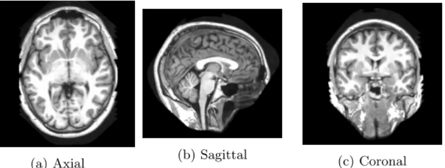
Nowadays we can obtain volume images so that we can get three different views from it:

• Axial plane. • Sagittal plane. • Coronal plane.

(11)

(a) Axial (b) Sagittal (c) Coronal Figure 2.1: Three different views from MR images. Many interesting properties of those image mentioned in [2] are: • Excellent capability for soft tissue structures.

• High resolution.

• High signal to noise ratio.

• Using different pulses we can get multi-channel images with variable con-trast; what can be used for segment and classify structures.

One of the problems we can find in MRI is the difficulty of obtaining uniform image quality. There are other problems such as being expensive and the need of spending time to take them.

2.2

Sub-cortical structures

Our brain is formed by several anatomical structures, cortical and sub-cortical structures [12].

The cortical structures are frontal lobe, parietal lobe, occipital lobe, tempo-ral lobe.

The Sub-cortical structures are hippocampus, cerebellum, amygdala, basal ganglia.

In this project we have been working with basal ganglia structure [11] whose main components are caudate nucleus and putamen (both of them form the structure called striatum), the globus pallidus, the subtantia nigra, the nucleus accumbens and the subthalamic nucleus. From those substructures we are per-forming the segmentation of the most important: caudate, putamen, globus pallidus and accumbens 2.2.

(12)

Figure 2.2: The four basal ganglia main structures manually segmented.: Cau-date,Putamen, Pallidum,Accumbens

2.3

Segmentation methods

Since manual labelling is a laborious task liable to inter and intra- variability depending on the clinical expert who does it and differences among subjects, it is desirable an automated technique to MRI segmentation There is still a challenge in developing faster and more accurate automatic segmentation despite the fact that many methods which can do that task exist.

In this section some methods are briefly explained in order to give an ap-proach for the state-of-the-art. This section is focused on magnetic resonance imaging segmentation methods giving more importance to those that are related with our proposal.

2.3.1

Atlas based

As it is said in [2] atlas based methods have outperformed other algorithms and those methods have had an increasing popularity. Unlike manual segmentation, atlas-based algorithms, as its name says, use atlases.

An atlas consist of two image volumes 2.3: • Template which is an intensity image • Labelled image which is a segmented image

(13)

Figure 2.3: On the left side we show an MR image and on the right side the corresponding labelled atlas [2].

The target image is registered with the template and then labels are propa-gatedto obtain the segmentation. Hence we have a registration problem.

The process is performed in two steps. A global registration for an initial alignment and a local registration for specific deformations. Registration has a high computation cost because it involves a complex discrete optimisation prob-lem [2]. To carry out the segmentation process of the target image these label propagation is performed which consists of transforming the manual labelling of the atlas using the mapping determined during registration. This process might fail if the target volume differs too much from the atlas resulting in a poor segmentation.

The paperBrainGraph: tissue segmentation using the Geodesic In-formation Flows framework. M. Jorge Cardoso, Marc Modat, and Sebastien Ourselin. UCL Centre for Medical Image Computing, London, UK included in the SATA Challenge [14] shows a new framework for tissue segmentation. Pop-ulation tissue priors are very important for an accurate segmentation. However, local brain different morphologies, algorithmic limitations in registration and mapping from each subject to a group-wise space is error prone.

In this framework [14], morphological similarity between pairs of images in a population it is used as a Markov Random Field constraint in the segmentation algorithm. This can be interpreted as an iterative generation of highly adapted subject specific priors from the locally most similar images in the database so that a population smoothness in segmentation procedure is introduced with-out the use of group-wise priors. This performance allows to segment subjects morphologically very different from the training set.

(14)

2.3.2

Multi-atlas label system

Segmentation errors produced by atlas-based methods are classified into sys-tematic errors and random errors [3].

Systematic errors are those which occur consistently, they usually describe a systematic pattern between automatic and manual segmentation. Systematic errors might be caused by errors in the registration process, partial volume effects or bias in manual labelling of atlases. One example of systematic error could be under-segmentation which consists of making the segmented structure a bit smaller than the manually segmented, for example due to a different criterion while assigning labels to a voxel.

Random errors are those which might be caused by image noise or subject variation. To reduce random errors we can use multiple atlases or selecting the most similar atlases for a given image. While using multiple atlases we can capture the variability of target regions better than if we only use one single atlas. When performing multi-atlas methods, a set of atlases is registered pairwise to the target image in order to being able to perform label propagation, after that, all propagated atlas labels are fused to generate the segmentation result. This method corrects a high amount of random errors which appear during registration resulting in a more accurate segmentation. Some of multi-atlas based methods are based on similarity among registered multi-atlases for a target image.

There are other performing strategies such as combination of several seg-mentations and refine it iteratively, those strategies do not consider the quality of the image registration. Atlas selection strategies depending on the informa-tion an atlas can contain and stopping when no improvement is expected and so on [2]. The problem of atlas selection strategies is that requires atlases to be registered first.

Label fusion strategies have shown an improvement in results too. That fu-sion takes part at the voxel level using one of the strategies: nearest neighbours, linear interpolation, majority voting, etc. A limitation of label fusing methods is that weights are computed independently for each atlas. This approach is sensitive to registration error too. To solve that it has been proposed local weighting voting.

We can conclude that multi atlas segmentation requires a pairwise accurate registration between atlas and target which is computationally expensive.

In fusion of multiple segmentation results, such as multi-atlas based algo-rithms, a majority vote is used as the basis of comparison of segmentation accuracy [14]. In the paper which appears in [14] a tailored majority method is shown. It improves the majority vote by choosing a threshold value that deviates from 50%, a number which is usually used in majority voting. At least 50% of voxels of the contributing segmentations indicates the class of the target voxel. This technique is applied in multi-atlas based methods.

This method it is also called ”flexible majority” where ”x% or more of the results agree” in the fused label vote where ”x” is called ”tailored majority vote value” and this performance is shown to out performs the traditional majority

(15)

vote. This value can be found by using the Dice similarity Coefficient of the overlap between ground truth and target image [14].

2.3.3

Intensity based: Combined global-local intensity

mix-ture model

Intensity based methods which use classifiers, rely on contrast between tissue types in feature space and adequate signal compared to image noise [14]. Sta-tistically an optimal boundary is identified to separate two tissue classes.

Many methods are proposed combining multi-atlas and intensity based in order to increase segmentation accuracy due to the fact that systematic errors occur consistently and, for some of them, is relatively easy to capture patterns correlated to them.

A method which works in that way is proposed in a paper found in [14]. That method consists of combining the patient global intensity with a population local intensity model.

2.3.4

Learning based

In order to reduce systematic errors some proposed works combine multi-atlas segmentation and learning-based methods [2]. If we suppose that the majority of systematic errors in segmentation occur consistently from subject to subject, then we can apply a wrapper method which try to learn intensity, spatial and contextual patterns associated to those errors. The wrapper method attempts to correct these systematic errors.

2.3.5

Patch based

The accuracy of non-rigid registration, fusion rules, selection of labelled images and labelling errors in manual segmentation are many key-points of registration-based label propagation [2].

Different from multi-atlas based, patch-based methods use local similar can-didates, called image patches, to estimate labels. As it is explained in [3] these methods obtain a label for every voxel by using similar image patches from coarsely aligned atlases. Image patches are extracted in a predefined neigh-bourhood around a voxel. According to the similarity of target patch and atlas patches, is given a weight to that patch. The final label of the target voxel is given by fusing the labels of central voxels of every patch. Using these non-local patch-based segmentation we can avoid the need of accurate non-rigid registra-tion so that we can get more computaregistra-tional efficiency.

However, image similarities over small image patches might not be an opti-mal estimator [3].

(16)

2.3.6

Reconstruction based

In [3] a segmentation method based on image patch reconstruction using discrim-inative dictionary learning [4] is proposed. Different from the idea of comparing the similarity between patches it uses a dictionary and a linear classifier which is learned from a template patch library for every voxel in the target image.

The surrounding patch to the target voxel can be reconstructed thanks to the dictionary and the label of the voxel is estimated by the classifier. As it is said in [3] the dictionaries can be learned offline and segment online.

Note that non-local assumption means that central voxel of similar patches belong to the same structure so that similar patches contribute to a better result.

2.3.7

Registration methods

ANTs System

Since many methods need an accurate registration of templates, this process has become an important challenge. In [14] the ANTs System is proposed for image registration. These registrations consist of an initial transformation, the identity if it is possible, of the image followed by several registration stages with increasing degrees of freedom. Each stage begins withksimilarity metric defini-tions with many multi-resolution strategy parameters. Then subsequent stages are added in the same way. Finally many optimisation options and pre/post-processing details are taken by ANTs.

Discrete optimisation

Discrete optimisation is a technique used in registration-based segmentation propagation.

In the paper Uncertainty Estimates for Improved Accuracy of Registration-Based Segmentation Propagation using Discrete Optimisation.

Mat-tias P. Heinrich, Ivor J.A. Simpson, Mark Jenkinson, Sir Michael Brady, and Julia A.Schnabel. Institute of Biomedical Engineering, Department of Engineer-ing, University of Oxford, UK. Oxford University Centre for Functional MRI of the Brain, UK. Centre for Medical Image Computing, University College Lon-don, UK. Department of Oncology, University of Oxford, UK contained in the SATA Challenge [14] it is described a method which incorporates uncertainty es-timates which are evaluated over the space of possible transformations. Optimal marginals distributions for a large range of local displacements are calculated which can be converted into probabilities. These probabilities, information of uncertainty, can be used to improve segmentation accuracy.

(17)

Chapter 3

Multi-Class Discriminative

Dictionary Learning

Segmentation and Stacked

Learning

3.1

Sparse representation classification and

dis-criminative dictionary learning

The searching for sparse coding of signals has been increasing in recent years. It has been shown that sparse representation provides a high performance in several applications such as image denoising, image painting and image com-pression [2]. This idea has also been used for methods in pattern classification such as in the Support Vector Machine where sparsity can be related to learn-ability of an estimator.

The aim of sparse representation is to reconstruct an input signal, for ex-ample an image patch, as a linear combination of a reduced number of signals taken from a dictionary.

Lety ∈Rn _{be signal. Let} _D _∈_Rn×k _{an over-complete dictionary (k > n)} where each column is calledatom.

We can obtain a representation ofy by the following linear system:

y=Dα (3.1)

Whereα∈RK _{is the sparse code of the signal}_y. α=argminαky−Dαk2

2 subject tokαk0≤T (3.2) BeingT a sparsity constraint andky−Dαk2

2≤reconstruction error and an error tolerance.

(18)

As a mesure of sparsity they suggest the`0 pseudo-norm1 [2, 5].

Hence we have a minimisation problem which is NP-hard but we can find suboptimals solutions by iterative methods. Since`0 is not convex, the`1is de closest convex function to carry out that minimisation, it was shown that both are equivalent as it is said in [2] if they are sufficiently sparse.

ˆ

α=argminαky−Dαk22 subject tokαk1≤T (3.3) Using the Lagrangian method, we can rewrite the problem as follows:

ˆ

y=minα 1

2 ky−Dαk 2

2 + λkαk1 (3.4)

where λkαk1 is the sparsity-inducing regularisation and λ > 0 is the La-grangian multiplier which balances the trade-off between reconstruction error and sparsity.

This equation (4) can be solved by several sparse coding methods [2]. Equa-tion (4) is solved using the Lasso2 _{method [2] in this case.}

Two issues to be aware of in the sparse coding model are the sparsity con-straint and whether the squared loss term is effective enough to characterize the signal fidelity [2].

Although the sparse representation is a good way for an accurately recon-struction of a signalysuch as denoising and image inpainting, for classification is more important if it is discriminative or not for the given signal classes than a small reconstruction error. Recently it has been shown that sparse represen-tation classification (SRC) has been successful in image processing and texture classification and face recognition [2, 4, 5].

In SRC, the target sample is represented as a sparse linear combination of the training samples [2]. Similar samples can be combined to make approximately a sample from the same class due to the fact that, in classification terms, samples from a single class lie on a linear subspace approximately meanwhile the rest cannot offer a linear representation as compact as the ones from the target sample class. That is why it can be said that SRC can be discriminative.

The sparse codeαcan be used as a feature for classification [5].

Given a set of signals Y = [y1, ..., yN] we assume that a dictionaryD that gave rise to the given signal examples via sparse representation exists and solves (1) for each signalyi given its sparse codingαi. Now we could wonder how can D be recovered? There exist many algorithm to solve that such as method of optimal directions[2] and K-SVD algorithm [2, 4, 5]. Both methods are iterative approaches designed to minimise

minα,Dky−Dαk2

2 subject tokαk0≤T, (3.5) and find the optimal dictionary.

First of all a dictionary D is initialised, then we have a loop composed of two stages [2]:

1_The_`0_{pseudo-norm of a vector is the number of nonzero coefficients of that vector.} 2_{Least absolute shrinkage and selection operator [15]}

(19)

1. Sparse coding: Fixed D we fin the best sparse decomposition of each signal as we saw before. 2. Dictionary update: here we find a difference between K-SVD and MOD. In MOD, the decompositionsαi are fixed and a least square problem solved updating all atoms simultaneously. In K-SVD, values of non-zero coefficients in theαiare not fixed and are updated at the same time as D. K-SVD receive its name from K-means.

The problem of K-SVD is that is not suitable for classification due to the fact that dictionaries must be representative and discriminative.

It has been developed a D-KSVD (discriminative K-SVD) [4] that uses labels of training data to incorporate a classifier into K-SVD and extends it by incor-porating the classification error into the objective function. The complexity of the method is bounded to K-SVD complexity.

D-KSVD solves the next problem:

hD, W, αi=argminD,W,αkY −Dαk2

2+ λkH−W αk22 (3.6) +βkWk2

2subject tokαk0 ≤T,

where W ∈ Rc×k _{are parameters for a linear classifier} _W ₌_H _∗_{α. Each} column ofH ∈Rc×N _{is a} _hi _{= [0, ...,}_{1, ...0], where non-zero position indicates} the class, beingcthe number of classes. The term involvingH is the classifica-tion error and kWk2 is the regularisation penalty. Those two terms should be minimised, hence we have a multivariate ridge regression problem [2, 4].

General steps for the Baseline Algorithm [4]: 1. InitialiseD andαusing K-SVD solving (5). 2. CalculateW whenDandαare fixed. 3. CalculateαwhenD andW are fixed. 4. CalculateD whenαandW are fixed. 5. Iterate 2 to 4 until some criterion are met.

But this Baseline algorithm can only find an approximate solution to (6) because in each step it finds a solution for every subproblem in the equation.

The problem can be rewritten as follow [3]:

hD, W, αi=argminD,W,αk PL √ β1H − D √ β1W αk2 2 (3.7) +β2kWk22subject tokαk0 ≤T

wherePL=Y which corresponds to patches (patch library, what we called set of signals before) and scalarsβ1andβ2 are parameters controlling the con-tribution of each term.

(20)

ˆ

αt=argminα_tkpt−Dtαtkˆ 2

2+λ2kαk1 (3.8)

where pt is the target patch (yi signal), ˆDt dictionary for the target patch andαt the target patch sparse decomposition.

Classification of target patch [3, 4, 5]:

ht= ˆWtαˆt (3.9)

where ht = [0, ...,1, ...,0] should have ideally one none-zero element which indicates voxels class.

Labelling:

vt=argmaxjht(j), j= 1, ..., C (3.10)

3.2

Segmentation by using multi-class

discrimi-native dictionary learning with label

consis-tency

In multi-class dictionary learning we focus in reconstruction [2], it is assumed that the target patch (the one that is being labelled) can be represented by a few template patches from the same structure as it is explained in sparse representation, represented by a few representative atoms from the dictionary. Two phases for labelling a voxel: coding and classification.

In discriminative dictionary learning, each voxel could be classified in two different classes: structure or background (not in the desired structure). In multi-class discriminative dictionary learning the number of classes to which a voxel can belong are more than two, several structures and the background (any desired structure). Hence H matrix has more rows than before, one for each class.

What is important now is the new constraint added, the label consistency, called discriminative sparse code error which is added to the objective function:

hD, W, A, αi=argminD,W,A,αkPL−Dαk2+ β1kH−W αk2 (3.11) +β2kQ−Aαk22+β3kWk2 subject tokαk0 ≤T,

where Q∈ Rk×N _{allows to specialise some atoms in the patches of a} par-ticular class due to the fact that they are the ”discriminative” sparse codes for the signals. It happens if the non-zero values for everyqi∈Rk _{occur where the} input signalyi and the dictionary itemsdk share the same label.

(21)

Figure 3.1: Q matrix: Atomsd1andd2 specialised in patchesp1 andp2 of one class, atomsd3 andd4 specialised in patchesp3−p7 of another class and atomsd5 andd6 specialised in patchesp8−p10of the last class:

Matrix A is a linear transformation matrix which transforms the original sparse codesαi to be most discriminative in feature spaceRk.Hence the term which involve Q and A represents de discriminative sparse-code error which enforce the sparse codesα since it forces the signals from same class to have similar sparse codes [5].

Therefore the unbalance problem is smoothed.

Figure 3.2: Unbalance problem: We can find it in boundary voxels where the number of structure patches and background patches in the patch library for the target voxel is unbalanced.

Learning and labelling proceeds as they do in DDLS. In the paper [5] an-other way of performing the label consistent K-SVD is shown where a linear predictive classifier is usedf(α;W) =W αwhich we mentioned before. Hence, both classifier and label consistency are applied in order to obtain a better performance.

3.3

Stacked Sequential Learning

In the MDDLS method we classify each voxel independently of its neighbours. In other words, we are not considering the classification of neighbours for classifying

(22)

the target voxel. In order to add this valuable information we consider a second stage inspired in Stacked Sequential Learning (SSL).

In this section we are reviewing briefly to Stacked Sequential Learning (SSL) [13, 16].

Despite of their values, neighbour data labels have inherent relationships in many classification problems. Sequential learning takes profit of this fact [13]. Contextual information is useful to solve ambiguous cases in classification.

Sequential learning is a meta-learning method 3_{in which an arbitrary base} learner is augmented, in this case by making it aware of its neighbourhood labels [16]. Standard classification assumes that samples are independently and identically drawn from a distribution of samples and their labels. Despite this fact, problems in real world can break this assumption.

Stacked sequential learning scheme is based in a two layers classifier. First of all a classifier is trained and tested with the original data set, then it is created an extended data set using the original data with predicted labels from the classifier added. A second classifier is training with this data which gives the final predicted labels. This approach shouldn’t be used for problems with a long range sequential relationship because the size of the extended data set increases exponentially. Sequential learning has been addressed from different perspectives such as graphical models, Hidden Markov Models or Conditional Random Fields read [13, 16] for more information about those points of view since we are focusing on meta-learning view which also includes sliding windows and recurrent windows techniques [13, 16].

As it is explained in [16], sequential learning can be applied to multi-class problems. Hence it is needed that classifiers have to be able to deal with mul-tiple classes. Another approach could be decomposing the problem in several binary problems and combine results. Here we find the problem on how can we decompose it in an efficient way and how can we combine the results we obtain. There is also a generalised version of stacked sequential learning which in-cludes a new block in its pipeline. As before, first of all a classifier is trained. Now appears the difference, the new block defines how the neighbourhood model of predicted labels is created. This block consists of a function which catches the data interaction with a parametrised model in a neighbourhood. Its output is added to the original data to create the extended features which are used to train the second classifier [13, 16].

Four more extensions for multi-scale stacked sequential learning (MSSL) are shown in [16], extension by likelihoods, learning objects at multiple scales, multi-class MSSL and extended data set grouping.

3_{A meta-learning technique uses a combination of different classifiers in order to predict a}

(23)

Chapter 4

Stacked Sequential

Multi-class Discriminative

Dictionary Learning for

MRI Segmentation

In this work, the objective is to segment the basal ganglia structure and four of its sub-structures [11, 12]. We apply MDDLS (multi-class DDLS) method as a first stage, then we incorporate more information obtained from MDDLS to classify each voxel applying Stacked Sequential Learning as a second stage (SS-MDDLS).

4.1

First stage: MDDLS

The first stage is formed by several steps in order to perform a multi-class discriminative dictionary learning (MDDLS) for magnetic resonance images. Sparse representation code (SRC) and binary discriminative dictionary learning (DDLS) methods for segment those images have been performed too [2]. Those steps are:

1. Initialisation and set default parameters.

2. Preprocessing, which consists of four sub-steps [23, 24]. 3. Building target crop.

4. Library and reduced library construction. 5. Perform segmentation.

(24)

7. Inverting registration

Except the segmentation step (step 5), the other steps are common for each method SRC, DDLS and MDDLS.

4.1.1

Initialisation

In this first step the initialisation is performed, default parameters are set, structures are created and tools are included.

We define parameters such as structures and sub-structures to segment with their labels value. The template for the registration process is chosen. So are the number of best atlases, patch and windows size, sampling step, neighbour-hood size parameters which is explained in the corresponding section. All those parameters are used by the subsequent pipeline steps.

4.1.2

Preprocessing pipeline

In this step, images are prepared for their segmentation. This step is composed by four sub-steps [23, 24]:

• Denoising

• Non-Uniformity correction • Registration

• Intensity standardisation

This preprocessing step is performed in order to solve, or at least to reduce, many problems in MRI such as variability caused by image formation.

In order to perform these operations properly, first of all, images should be aligned resetting coordinates.

(25)

Figure 4.1: Example of resetting coordinates to the origin [2]. Denoising

The problem of noise is closely related to MRI system and it is know that it has a Rician distribution [2, 24].

So that, the denoising step is very important. This step increases image quality to improve subsequent steps performance for quantitative analysis.

Denoising methods applied in this performance are 3D block-wise non-local means filter [2]. To reduce the noise in the image, redundant information is used by the filter despite being more difficult to carry out in 3D images than 2D. For reducing the noise a method based on Median Absolute Deviation estimator for Rician noise [2] is used.

Once this step is done, we obtain denoised images which are used by the next step, the non-uniformity correction.

Non-Uniformity correction

Non-uniformity correction tries to reduce the intensity inhomogeneity problem also called bias field or shading artifact. In radio frequency, the non-uniformity when we obtain data might produce a shading effect. This effect is harmful due to the fact that affects to the qualitative and quantitative analysis of images.

(26)

The main feature of this effect is the variability of intensity value for voxels from the same tissue. That is why this issue has become an important problem to be aware of and to solve. This effect can appear for many reasons such as regular calibration or several subject properties. This effect can appear inter-and intra-slice.

To ensure that each tissue has the same intensity within a single image it is used the N3 (non parametric, non uniform, normalisation) intensity non-uniformity correction of Sled [2].

These images are used for registration step. Registration

First of all, register two images means align them in order to make to see over-lapping or differences among their common features. In this process a geometric transformation is performed. This problem is composed by four main compo-nents [2]:

• Feature space. Determine what is registered. Algorithm used is feature dependent.

• Search space. Consider two images (the two that we want to register) as two functionsf(x) andg(x) inRn _where_n_{= 1,}_{2, to align them a} trans-formationT(y) has to be found, this transformation must accomplish the next condition: f(x) =T(g(x))∀xsupposing that g(x) =y. There exist rigid transformation such as translation and rotation or affine transforma-tion for example to consider different scales. So the search space is the type of transformation we choose.

• Search strategy. Once the search space is chosen a transformation and their subsequent transformations have to be chosen.

• Metric similarity. Measure how good isf(x) compared toT(g(x)). Mean-square error, correlation, etc.

Two categories for registration, rigid and non-rigid (affine) as it was said before. In this case an affine registration is applied for all our subjects [2] registered to the MNI-ICBM152 template. Same registration is applied for ground-truth (expert manually segmented images). This template is provided by Montreal Neurological Institute created by using data from ICBM project [2].

These resulting images are used by the next step. Intensity standardisation

The grey scale for MR images is not standard, this problem might cause a lack of tissue specification within the MRI protocol, for the same body region, same patient, etc. Therefore intensity measures cannot be associated to an anatomical

(27)

meaning. So that a standardisation process has to be preformed. However, only few works have addressed this problem [2].

Those methods try to correct inter-subject intensity variations standardising the grey scale in this case a 0 to 255 scale using a 1-D histogram matching approach [2]. first by calculating percentiles on the template and the reference histogram then they are matched by linear interpolation between locations. So that, similar tissues obtain a similar value.

Finally, images are ready to be segmented.

4.1.3

Building Image crop

We are only extracting a part from the image, that part consists of the region where we can find the structure to segment, so that we do not need to segment the whole image. This process is carried out by calculating masks and bounding box. Once we have them, we can extract a sub-volume for every subject. Masks and Bounding Box creation

During this step masks and bounding boxes for every structure and sub-structure are created.

Using the ground truth images (images manually segmented by an expert) we obtain the boundaries for every structure for the subjects of training. We can also apply this step to test subjects due to the fact that we have their respective ground truth images and this information is used later for analysis. Once we have them, they are merged into a bigger mask which delimits a region of the image where the structure (or substructure) is contained. We can ensure this fact because of the use of many ground truth images. As more subjects are used, better is that region.

The process which is used is simple, the union of all structure (or sub-structure) regions creates the final mask [2]. From these masks (one for every structure and substructure) we obtain the bounding box which is formed by co-ordinates which delimit the mask: initialxcoordinatex1, finalxcoordinatex2, initialycoordinatey1, finalycoordinatey2, initialzcoordinatez1, finalz coor-dinatez2. This information is saved matching every structure and substructure with their respective bounding box (BB).

These information is used later to analyse and show results.

4.1.4

Library construction

Centroids generation

Centroids (or target voxels) are the voxels that are used during the segmentation process and during the second stage. Those voxels are chosen by a step sample. For instance, if the step sample is 3 means that one voxel is chosen for every three.

Those voxels are defined in cropped images obtained in the previous state, so that, their coordinates correspond to the cropped image region starting by

(28)

(1,1,1). Of course, it is sure that the target voxel belongs to the area delimited by the bounding box, so that it has relevant information.

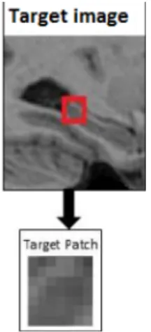
A patch of a determined size around the target voxel is a group of voxels around the target, or central, voxel. It is more understandable having a look at the image 4.2.

Figure 4.2: Patch creation from the cropped image (target image). The patch is marked by the red square. In this case is a 5×5×5 voxel group around a target voxel (central voxel) [3].

Patch library creation

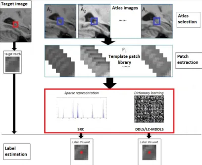
We have to create a patch library for every target voxel from the target image (the image we are labelling). The library is constructed by using theN most similar images from the training set. To find which images are the most similar, the squared intensity differences (SSD) method is used on the cropped image.

Hence, the first step is getting theN most similar subjects using SSD in the template space.

The next step is patch extraction, the target patch is denotedpt[2, 3]. For this extraction asearch volume consisting of a cube centred around the target voxel. The search volume is extracted for every similar subject, the cube is of sizep×p×pwhat is calledpatch size around the target voxel. If, for instance, p = 5, the patches are of size 125. Those extracted patches form the patch libraryPL.

We construct a patch libraryPL for every target voxel in the target image. Therefore our patch library contains thousands of patches. It should be men-tioned too that this patch library is atlas-wise what means that is created for every target voxel for each atlas [2].

The patch library PL can be represented as follows: PL= [p1, p2, ..., pn]∈Rm×n_,

(29)

wherepiis a patch,mthe patch size andnthe number of patches that form the library.

Figure 4.3: Flow chart for the labelling. Red square represents the patch and the blue square represents the search volume. The target image corresponds to the image to label and the target voxel the central voxel from the target patch. Atlas images correspond to the training set images. [3]

4.1.5

Dictionary construction

At this step we find the differences among the three methods: sparse represen-tation classification, discriminative dictionary learning and label consistency. Sparse representation based classification

This method uses the whole patch libraryPL as a predefined dictionary for the sparse coding. So we can represent the target patchpt, using elements from the library, approximately as follows:

pt=α1p1+α2p2+...+αnpn,

since it is sparse, the majority of the coefficients αi are zero. The problem is that this dictionary has too much redundancy and it makes the process take more time. The idea is that non-zero coefficients should concentrate on patches of the same class (more similar). That fact is due to the sparsity and the use of all classes while computing coefficients [2, 3]. Look at section 3.1 for more details.

(30)

Discriminative dictionary learning and label consistency

Learning a compact dictionary for each individual target patch is better than using the whole patch library as a predefined dictionary due to its drawbacks. Therefore, learning a new dictionary able to reconstruct and to be discriminative is a better option. In this case D-KSVD is used [4]. Hence, the objective function is:

hD, W, αi=argminD,W,αkPL−Dαk2+ β1kH−W αk2 (4.1) +β2kWk2 subject tokαk0 ≤T,

where each column of H is the label vector corresponding to a template patch, where the non-zero entry corresponds to the central voxel label from that patch.

As it was said before, D-KSVD uses K-SVD for finding an optimal solution simultaneously for all parameters [4]:

hD, W, αi=argminD,W,αk PL √ β1H − D √ β1W αk2 2 (4.2) +β2kWk2 2 subject tokαk0 ≤T We can rewrite it as follows:

hD, W, αi= arg min D,W,αk

˜

PL−Dαk2˜ (4.3)

subject tokαk0 ≤T

where ˜D= Dt,√β1Wttis normalised column-wise and ˜PL= P_Lt,√β1Htt which includes the original patch and its label. We can drop the penalty term.

As it says in [2, 3] a online dictionary learning algorithm is used to solve (5). Using ˜D a classifier ˆW and a learned dictionary ˆDare obtained [2, 4] com-puted as: ˆ D= ( ˜ d1 kd˜1k2 , ˜ d2 kd˜2k2 ,· · · , ˜ dk kd˜kk2 ) (4.4) ˆ W = _w1_˜ kw˜1k2, ˜ w2 kw˜2k2,· · ·, ˜ wk kw˜kk2 (4.5) See [4] for proof.

(31)

4.1.6

Perform segmentation

Sparse representation classification

As it was said before, the whole patch libraryPLis used as a dictionary. Hence the label value for the target voxel of the target patchpt(the central voxel defines the class of the whole patch) is assigned as the class with less reconstruction error:

vt=argminjrj(pt), ∀j = 1, ..., C, (4.6) whererj(pt) =kpt−P_Ljαˆj_k_{is the reconstruction error and}_αj _{the sparse} co-efficient of the classj. These coefficients are obtained using Elastic Net method [2, 3]: ˆ α=minα 1 2kpt−PLαk 2 2+λ1kαk1+ λ2 2 kαk 2 2 (4.7)

Discriminative dictionary learning

For labelling the target voxel it proceeds as we said in section 3.1. Using Lasso we obtain the sparse representation:

ˆ

αt=argminα_tkpt−Dtαtkˆ 2

2+λ2kαk1 (4.8)

And we estimate the final label:

ht= ˆWtαtˆ (4.9)

wherehtis the label vector of the central voxel from the target patch. The labelvtis the index of the largest element in that vector:

vt=argmaxj ht(j) (4.10) Label Consistent Multi-class DDLS

Due to the lack of handling unbalanced libraries that DDLS has, the label con-sistency multi-class discriminative dictionary learning is used as it is explained in 3.2. Therefore, matrixH has more rows due to the fact that now we have more classes, not only two.

Then, the function objective is the next one:

hD, W, A, αi=argminD,W,A,αkPL−Dαk2+ β1kH−W αk2 (4.11) +β2kQ−Aαk2

(32)

werekQ−Aαk2

2 is the label consistence regularisation term andQthe dis-criminative sparse codes of the input patches in the patch libraryPLfor classi-fication [2, 5].

The learning process is the same as used in DDLS but adding the label consistency term: hD, W, αi=argminD,W,αk   PL √ β1H √ β2Q  −   D √ β1W √ β2A  αk2+ (4.12) subject tokαk0 ≤T

And labelling is the same process as in DDLS [2].

4.2

Second stage: SS-MDDLS

In order to improve the performance we are proposing the next implementation which consists of a subsequent stage inspired by Stacked Sequential Learning [13, 16].

From the information we get from the linear classifier during the stage one, we are training another classifier for labelling the target voxels.

In DDLS and MDDLS we use the ht = Wtαt label vector to classify the target voxel whereW is the linear classifier andαthe sparse representation. So that we propose to use not only the target voxel vector but also the vectors of its nearest neighbours to classify it. Contextual information helps to classify the target voxel.For example a background voxel is surrounded by background voxels except for a voxel in a structure boundary, that is why contextual information can help to classify the target voxel.

So that we have a feature vector formed by seven differenthtvectors. One from the target voxel and the other six from its neighbours. We are getting the neighbours from right, left, up, down, front and rear having the target voxel as centre reference. Hence, the feature vector from the target voxelftis:

ft= [ht, h1,· · ·, h6],

where ht is the label vector of the target voxel andhi ∀i = 1,· · · ,6 the label vector of the neighbour voxels. In our case, eachhvector is formed byC (number of classes) components, one for each class, hence,ft∈R7∗C.

4.2.1

Classification

Once we have computed the feature vectors for all the samples, we use this data to train a new classifier using decision trees [20, 21]. Once we have done it, we classify the testing subjects using that trained classifier and we obtain the predicted label for every voxel.

(33)

Decision Tree Learning

The decision trees are a bootstrap aggregation for ensemble of decision trees for either classification or regression. In our case we are using this strategy for classification [20, 22].

Given a training data set and their class labels, which corresponds to the ground truth segmentation in our case, the algorithm trains a group of classifi-cation trees. Then algorithm works as follows [20]: It generates in-bag (observa-tions included in the decision tree) samples by oversampling classes with large miss-classification cost and under-sampling those with low miss-classification cost. So that out-of-bag (observations not included in the decision tree) sam-ples have fewer observations from classes with large miss-classification cost and more observations from the other classes. Every tree is grown on an indepen-dently drawn bootstrap replica of input data. An average of predictions from every individual tree is taken in order to compute the prediction for unseen data.

The method of Bagging predictor [22] generates multiple versions of a predic-tor and uses them to get an aggregated predicpredic-tor. When predicting a numerical outcome, the aggregation averages over the versions and does a majority vote to predict the final class. As it is said in [22], the multiple versions are formed by making bootstrap replicates of the learning set and using them as the new learning set.

The proof about why does Bagging predictor work can be found at [22] as well as a more mathematically oriented explanation of classification and regression using Bagging predictor.

4.2.2

Extended Feature Vector

In order to help to learn contextual patterns, we propose to use an extended feature vector.

In this case we add toftthe sparse representationα. Hence, we create this new feature vector:

f_t0= [ht, h1,· · ·, h6, αt, α1,· · · , α6],

where αt corresponds to the sparse representation for the target voxel and αi ∀i= 1,· · ·,6 are the sparse representations from its six neighbours.

Since we work on a crop from the image, we might find that a neighbour is out of the bounding box. We know that it is a background voxel, therefore, as we did before, we impose a feature for this type of voxels. So that, we add [1,0,· · ·,0] as theirα.

Each α ∈ RK _{(see section 3.1) where} _K _{is the number of atoms of the} dictionary, then we add 7∗K features to the feature vector.. Hence, our new f_t0∈_R7∗(C+K)_.

The big size of the new feature matrixF∈Rn×m_where_n_{is the number of} centroids (target voxels) andmthe size off_t0 we decide to use a sub-sampling of voxels. This sub-sampling gets 1 for every 3 voxels in each dimension. Then, we

(34)

reduce the size of that matrix. It should be mentioned that despite having fewer voxels than before, we still have information about almost every voxel from the cropped image (target image) since we use information from neighbours. Therefore, we have less training observations but we have more information from them.

4.3

Matlab

Matlab [17] is a high level language which allows the user to explore and visualise data as well as image and signal processing, communication, control systems and computational finances.

This language has many useful features such as:

1. Numerical calculations: Matlab offers several numerical methods which allow to perform engineering and scientific operations whose functions are optimised in order to make vectorial and matricial calculus fast.

2. Data analysis and visualisation: Many tools are offered by matlab to ob-tain, analyse and visualise data to make those tasks faster.

3. Algorithm development and programming: since it is a high level language it allows to develop algorithms using many tools which help to do it faster. An important part is vector and matrices support.

4. Applications development and distribution: Many tools are given by mat-lab to make easier application sharing and distribution.

After this brief approach to Matlab we have chosen this development lan-guage due to the tools it offers which are very useful for imaging management because of its vector and matricial support. A part from that we also found useful the fact that many data analysis and visualisation tools which are really helpful for our purposes. Points 1, 2 and 3 are which we found more suitable for what we need.

4.4

Statistical parametric mapping

The Statistical Parametric Mapping (SPM) package is used for construction and assessment of spatially extended statistical processes used to test about imaging data [18]. It has been designed for the analysis of brain imaging data sequences as MRI.

More detailed information can be found in [18, 19].

It is voxel based. It allows to realign images, spatially normalise and smoothen them. Uses General Linear Model to describe data. SPM uses classical statis-tical inference where multiple comparisons problem is addressed using random field theory under many assumptions. It can also use Bayesian inference.

(35)

This package is helpful during the preprocessing period, when images are previously preprocessed in order to reduce noise, normalise intensity among subjects and image registration to a stereotaxic space.

4.5

Code details

An important structure is created during centroids generation process, a struc-ture which contain the coordinates from every target voxeln−centroids×3, coordinates from a reduced number of voxelsm−centroids×3 with their se-quential indexes in the image m−centroids×1 and matrix containing the patches, their initial coordinates, for every centroid.

Patch libraryPLis a matrix where patches are grouped column-wise. Hence, every column ofPL is a different patch.

To construct the feature vector we use a structure created during MD-DLS segmentation. That structure contains coordinates of target voxels in the cropped image (all of them)centroidM at∈Rn×3_where_n_{is the number of} tar-get voxels, coordinates of a sampling of those voxels (reducedM at∈Rl×3_where lis the number of sampling) in addition to their sequential index (idxReduced∈

Rl_{) in the cropped image and the patch library.} Steps:

1. Obtaining data. At first we obtain the h vector for every target voxel. This information is obtained while performing MDDLS segmentation. 2. Search neighbours. Then we look for the six neighbours for every target

voxel and discern which ones are inside the bounding box and which ones are out of it.

3. Fill feature matrix. Feature matrix F ∈ Rn×m _where _n _{is the number} of target voxels and m=ftsize. Therefore, columns are the features for every voxel whose mapping is ith-row corresponds to the feature vector of the ith-target voxel in centroidM atmatrix. Hence we fill each row of F using the label vector from the target voxel and its neighbours label vectors.It should be mentioned that we have the label vector from every voxel, voxels out of the bounding box are, for sure, background voxels so that their label vector is ht = [1,0,0,0,0] and voxels label vector from the cropped image (target image) has been computed when performing MDDLS segmentation.

Once we have the feature matrix completely filled for every subject, we mix every feature matrix into a single feature matrix which we called Xtrain ∈

R(n∗k)×m _where _n_{is the number of target voxels,} _k _{is the number of training} subjects (in our case k = 28) and m = sizeft the size of the feature vector, in this casem = 35 since it contains the ht ∈ R5 _{of seven voxels (target and} six neighbours). Since it is the training set, we know their correspondent label so that we obtain them from the manually segmented image using coordinates given incentroidM at.

(36)

The extended feature vector f_t0 ∈R595_{; 595 = 7}_∗_{(5 + 80) where 7 is the} number of subjects whose data used, the target plus its six neighbours,C= 5 the number of different classes andK= 80 the number of atoms of the dictionaries.

(37)

Chapter 5

Experiments

In this section we expose the performance of the different methods presented. We replicate SRC, DDLS results applied to the four structures from the basal ganglia and a brief comparison between them[1, 2]. In addition we analyse the results obtained from MDDLS. To finish we are showing the performance of SS-MDDLS and a comparative analysis of the obtained results.

5.1

Dataset

For this performance we are using MR images from 35 different subjects. The same dataset as it is used in [2]. The 35 subjects and their corresponding segmentation were made public by the MICCAI 2012 Grand Challenge and Workshop on Multi-Atlas Labelling. The data-set images (corresponding to both training and test) for distinct human data consist of a de-faced T1-weighted structural MRI and its associated manually labelled volume with one label per voxel. Each volume (MRI and label) is stored in a separate 3D NiFTI1 file.

The original MRI scans were obtained from the OASIS project http:// www.oasis-brains.org/. The specific scans used were from a subset of the

Crossectional MRI Data in Young, Middle Aged, Non-demented and Demented Older Adultcalled ”reliability data”. Here, 35 normal control volunteer subjects were each scanned twice. They were all right handed and include 13 males and 22 females. Their ages ranged from 19 to 90 with an average of 32.4 years old.

5.2

Methods and parameters

Four different methods have been used. From which the fourth is our proposal. • SRC. See section 3.1.

• DDLS. See section 3.1. 1_{http://nifti.nimh.nih.gov}

(38)

• MDDLS. See sections 3.2 and 4.1. • SS-MDDLS. See section 4.2.

General parameters setting as used in [2]: • Bounding box padding: 3

• Best subjects: 8 • Patch size: 5 • Window size: 3 • Sampling step: 3 • Dictionary atoms: 80 • Neighbours: 6 • C (number of classes) = 5 DDLS and MDDLS parameters; • Lambda: 0.15 • Lambda2: 0 • Iterations: 40 • Mode: 5

• Positive constraint on coefficients: true • Mode D: 0 (non-sparsity in dictionary atoms) • Positive constraint on dictionary: true • Batch size: 25

• Iteration update: 1 • Mode parameter: 0 SS-MDDLS parameters;

• Number of decision trees: 50, 100, 200 • Neighbours distance: 1, 6

(39)

5.3

Evaluation

The evaluation strategy is a nested cross validation. First, we split our dataset in two groups, training set and test set. We use the training set for learning dictionaries and classifiers for MDDLS and SS-MDDLS. Then we segment the test set using using those methods. Our dataset is formed by 35 subjects. Hence, our training set consists of 28 subjects and our test set consists of 7 subjects. We make five different combinations of this two subgroups in order to have all subjects as test subject once.

As an evaluation measure we have computed the Dice coefficient between manually segmented images and automatic segmentation. This overlap coeffi-cient, also known as kappa coefficoeffi-cient, is computed as follows:

For two binary segmentationAandB, the Dice coefficient is computed as: κ(A, B) = 2|A∩B|

|A|+|B| (5.1)

5.4

Results

In this section, we show a comparative analysis of the obtained results. At first we introduce SRC and DDLS results and then we discuss about MDDLS and SS-MDDLS performance.

5.4.1

SRC and DDLS results

At first we replicate results in [2] just to have an initial approach of segmentation results applied to MRI and to briefly analyse SRC and DDLS performances.

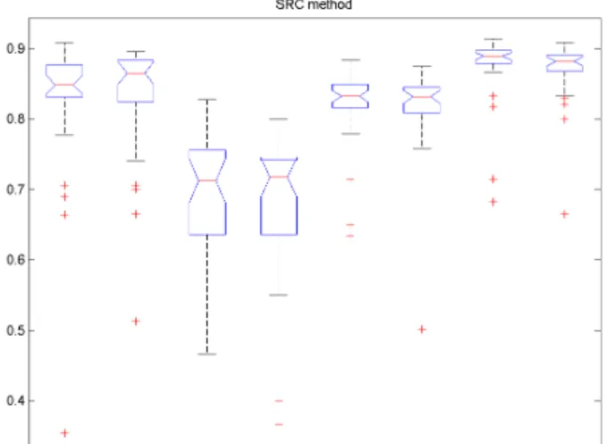
As we can see in figures 5.1 5.2, DDLS method has a better performance than SRC since its overlap indexes are much higher. We can also notice that standard deviation is higher in SRC than in MDDLS so that, the overall accuracy is reduced.

It can be deducted that DDLS is more robust against subjects whose images are more different from the rest of the data-set. We can find this fact in the number of outliers. SRC has much more outlier subjects than DDLS what means, again, that SRC is outperformed by DDLS.

(40)

Figure 5.1: Boxplot showing overlap statistics for DDLS method for the four sub-structures from the Basal Ganglia.

Figure 5.2: Boxplot showing overlap statistics for SRC method for the four substruc-tures from the Basal Ganglia.

Let us see the results more accurately in the tables 5.1 and5.2. We split the results in two different tables to show left and right structures separately.

(41)

Caudate L Accumbens L Pallidum L Putamen L

SRC mean overlap 83% 69.7% 82.1% 87.6%

SRC deviation ±10% ±8.5% ±5.4% ±4.8% DDLS mean overlap 87.8% 75.7% 85.5% 90.4% DDLS deviation ±6.4% ±5.4% ±4.6% ±3.6% Table 5.1: Average Dice overlaps for Basal Ganglia (BG) left structures.

Caudate R Accumbens R Pallidum R Putamen R

SRC mean overlap 83.5% 67.8% 81.7% 87%

SRC deviation 8.1% 10% 6.1% 4.3%

DDLS mean overlap 88.5% 75.2% 85.8% 90.3%

DDLS deviation 4.4% 5.8% 5% 3.4%

Table 5.2: Average Dice overlaps for Basal Ganglia (BG) right structures. As we deduce from the boxplot figures and tables, DDLS results are much better than SRC results. DDLS not only has higher average results but also has a lesser standard deviation than SRC. Remember that SRC uses the sparse representation from voxels as a dictionary, meanwhile DDLS learns dictionaries for every voxels from the most similar subjects in the training set. This fact has been proved to improve performance in MRI segmentation.

Since DDLS has shown a better performance we do a further analysis of its results.

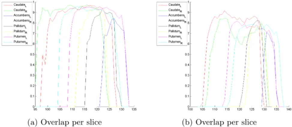
Until now we show the average overlap among all the training subjects. Then we study the overlap index per subject and per slice in order to make a more accurate analysis. Let us see a couple of examples in the figure 5.3:

(a) Overlap per slice (b) Overlap per slice

Figure 5.3: Overlap per slice. The image in (a) shows the overlap for a standard subject and the image in (b) a subject which is usually classified as outlier since the age of this subject is 90 years old. We can observe that, despite having different indexes, both have their overlap reduced at start and end slices.

(42)

We have noticed that the overlap has a lower index at the starting and ending slices. The overlap ratio is considerably lower at those slices than at central slices. It might be caused by the substructure morphology because starting slices are those where the structure is beginning and ending slices are those where the structure is disappearing. Hence, because of the fact that we use a training set, for several subjects the structure appears before than for others. This fact means that slices where the structure appears or disappears (border slices) are confusion areas since it is hard to distinguish if there is structure in that location or not. Figure 5.4 shows a qualitative example.

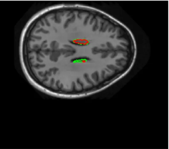
Figure 5.4: Axial view from a starting slice for the caudate segmentation where green is the manually segmented structure and red the automatic performing DDLS

We can describe this error as systematic since it is shown in every subject. These border slices are difficult to classify making the performance worse in those regions.

(43)

Figure 5.5: Axial view from a central slice for the caudate segmentation where green is the manually segmented structure and red the automatic performing DDLS

5.4.2

MDDLS results

In this new section we are showing more interesting results. MDDLS has a better performance than DDLS and SRC. So that we are studying these results more accurately.

First of all let us show an extended dice overlap table. Data has been split in two different tables due to the high amount of information. We show right hemisphere structures in 5.3 and left hemisphere structures in 5.4 substructures separately, as we did before. Averages are shown in 5.11.

(44)

Putamen R Caudate R Pallidum R Accumbens R 1000 3 R 0.911 0.901 0.846 0.774 1001 3 R 0.924 0.903 0.868 0.794 1002 3 R 0.906 0.891 0.863 0.711 1003 3 R 0.909 0.892 0.852 0.769 1004 3 R 0.922 0.899 0.856 0.769 1005 3 R 0.905 0.918 0.884 0.791 1006 3 R 0.914 0.914 0.907 0.785 1007 3 R 0.909 0.857 0.878 0.745 1008 3 R 0.923 0.897 0.873 0.783 1009 3 R 0.899 0.896 0.888 0.822 1010 3 R 0.920 0.871 0.863 0.688 1011 3 R 0.917 0.902 0.902 0.776 1012 3 R 0.881 0.882 0.856 0.805 1013 3 R 0.914 0.911 0.858 0.800 1014 3 R 0.874 0.898 0.868 0.712 1015 3 R 0.911 0.917 0.875 0.720 1017 3 R 0.798 0.781 0.740 0.479 1018 3 R 0.913 0.878 0.898 0.788 1019 3 R 0.913 0.884 0.875 0.791 1023 3 R 0.912 0.847 0.863 0.706 1024 3 R 0.925 0.904 0.863 0.821 1025 3 R 0.911 0.924 0.865 0.809 1036 3 R 0.899 0.898 0.843 0.787 1038 3 R 0.911 0.922 0.875 0.797 1039 3 R 0.911 0.886 0.882 0.747 1101 3 R 0.901 0.890 0.858 0.743 1104 3 R 0.916 0.899 0.864 0.767 1107 3 R 0.886 0.878 0.865 0.732 1110 3 R 0.903 0.878 0.885 0.785 1113 3 R 0.897 0.878 0.863 0.704 1116 3 R 0.896 0.856 0.856 0.614 1119 3 R 0.881 0.802 0.812 0.661 1122 3 R 0.897 0.817 0.873 0.658 1125 3 R 0.906 0.645 0.872 0.800 1128 3 R 0.678 0.539 0.614 0.530

Table 5.3: Dice overlaps for Basal Ganglia (BG) Right substructures using MDDLS.

(45)

Putamen L Caudate L Pallidum L Accumbens L 1000 3 L 0.918 0.890 0.877 0.727 1001 3 L 0.926 0.903 0.876 0.765 1002 3 L 0.908 0.886 0.869 0.720 1003 3 L 0.919 0.888 0.881 0.771 1004 3 L 0.934 0.913 0.863 0.799 1005 3 L 0.919 0.903 0.882 0.803 1006 3 L 0.921 0.900 0.876 0.760 1007 3 L 0.905 0.849 0.844 0.764 1008 3 L 0.921 0.899 0.875 0.804 1009 3 L 0.913 0.883 0.881 0.764 1010 3 L 0.923 0.881 0.882 0.798 1011 3 L 0.918 0.895 0.879 0.798 1012 3 L 0.905 0.910 0.869 0.822 1013 3 L 0.911 0.901 0.845 0.813 1014 3 L 0.908 0.894 0.893 0.705 1015 3 L 0.880 0.900 0.872 0.817 1017 3 L 0.875 0.815 0.859 0.645 1018 3 L 0.921 0.890 0.876 0.811 1019 3 L 0.919 0.896 0.885 0.831 1023 3 L 0.896 0.864 0.819 0.723 1024 3 L 0.912 0.910 0.865 0.833 1025 3 L 0.912 0.909 0.839 0.786 1036 3 L 0.913 0.906 0.846 0.714 1038 3 L 0.917 0.925 0.882 0.861 1039 3 L 0.909 0.913 0.883 0.816 1101 3 L 0.917 0.886 0.892 0.736 1104 3 L 0.919 0.892 0.889 0.767 1107 3 L 0.892 0.873 0.861 0.656 1110 3 L 0.912 0.864 0.889 0.770 1113 3 L 0.919 0.889 0.887 0.741 1116 3 L 0.875 0.822 0.846 0.696 1119 3 L 0.798 0.400 0.783 0.750 1122 3 L 0.902 0.833 0.814 0.787 1125 3 L 0.826 0.676 0.746 0.806 1128 3 L 0.732 0.812 0.703 0.677

Table 5.4: Dice overlaps for Basal Ganglia (BG) Left substructures using MD-DLS.

As we can see, using MDDLS better results are obtained. Remember that it uses label consistency in order to reduce the unbalance problem. Hence, results have been slightly improved compared to DDLS.

5.4.3

Results analysis

Here we analyse the results visualising pseudo-probability maps and profiles of the first stage classification results.

(46)

While we perform MDDLS (sections 3.2, 4.1) in order to classify the target voxel (centroid) from a target patchpt we use a label vector ht=Wtαt where Wt is the lineal classifier for the target voxel andαt the sparse representation of the target voxel, sub-indextcorresponds totarget.

The final label of the target voxel, and consequently, the label of the target patch is obtained by:

vt=argmaxjht(j), j= 1, ..., C (5.2) Since it is not an ideal ht = [0, ...,1, ...0] with a one non-zero value which determines the label, we find interesting to study information given byht.

In order to visually analyse them we have defined the pseudo-probability maps as thesehtvalues of every voxel in an image crop.

For every subject we create this pseudo-probability map for each class, in this case five different probability maps. These maps allow us to visually compare ht vector values.

First of all we normalise ht vectors between 0 and 1 in order to have the same range for every map. For that we divide for the maximum of allhtvalues in the image.

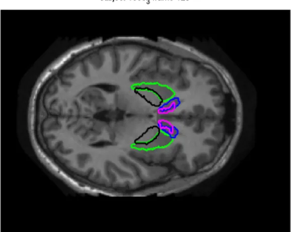
Our label vector has five different values. We have a ht for every voxel in the target image (the crop where the structure is contained). Hence, we create a matrix H ∈ R5×n _{where 5 is the number of classes (background, putamen,} caudate, pallidum, accumbens) andn is the number of target voxels, for every subject.

Using H we create five different mapsMi ∈Rm×k×l _∀i_{= 1,}_{· · ·}_,_{5 where} m,k,l, are the sizes of the target image and m∗k∗l=n. Then we fill every Mi using data from every i-th row ofH. In other words, the first value of every htfrom this subject fillsM1, the second fillsM2and so on, making coordinates to match. See figure 5.6 for an illustration.

Figure 5.6: Schema about howH matrix is used to create probability maps. Making each row to be a different map.

(47)

As a result we obtain the following maps in figures 5.7 5.8 5.9 5.10 5.11:

(a) Manual segmentation (b) MDDLS segmentation

Figure 5.7: Pseudo-probability maps where (a) has the manually segmented contour superposed and (b) the MDDLS contour superposed. Blue means the lowest probability for a voxel to belong to Putamen structure and Red the highest probability.

Figure 5.8: Pseudo-probability maps where (a) has the manually segmented contour superposed and (b) the MDDLS contour superposed. Blue means the lowest probability for a voxel to belong to Caudate structure and Red the highest probability.

(48)

Figure 5.9: Pseudo-probability maps where (a) has the manually segmented contour superposed and (b) the MDDLS contour superposed. Blue means the lowest probability for a voxel to belong to Pallidum structure and Red the highest probability.

Figure 5.10: Pseudo-probability maps where (a) has the manually segmented contour superposed and (b) the MDDLS contour superposed. Blue means the lowest probability for a voxel to belong to