State University of New York College at Buffalo - Buffalo State College
Digital Commons at Buffalo State
Applied Economics Theses Economics and Finance
8-2013
Forecasting Foreign Exchange Rates
Timothy M. Znaczko
STATE UNIVERSITY OF NEW YORK BUFFALO STATE, [email protected]
Advisor
Dr. Theodore F. Byrley, Chair and Associate Professor of Economics and Finance First Reader
Dr. Theodore F. Byrley, Chair and Associate Professor of Economics and Finance Second Reader
Dr. Ted Schmidt, Associate Professor of Economics and Finance Third Reader
Dr. Fred Floss, Professor of Ecnomics and Finance Department Chair
Dr. Theodore F. Byrley, Chair and Associate Professor of Economics and Finance
To learn more about the Economics and Finance Department and its educational programs, research, and resources, go tohttp://economics.buffalostate.edu/.
Follow this and additional works at:http://digitalcommons.buffalostate.edu/economics_theses
Part of theBusiness Administration, Management, and Operations Commons,Finance and Financial Management Commons, and the
International Business Commons
Recommended Citation
STATE UNIVERSITY OF NEW YORK COLLEGE AT BUFFALO
DEPARTMENT OF ECONOMICS AND FINANCE
FORECASTING FOREIGN EXCHANGE RATES
A THESIS IN
ECONOMICS AND FINANCE
BY
TIMOTHY M ZNACZKO
SUBMITTED IN PARTIAL FULFILLMENT OF THE REQUIREMENTS
FOR THE DEGREE OF
MASTER OF ARTS AUGUST 2013
Approved by:
Theodore F. Byrley, Ph.D. CFA
Chair and Associate Professor of Economics and Finance Chair of Committee
Thesis Advisor
Kevin J. Railey, Ph.D.
© Copyright by Timothy M Znaczko
THESIS COMMITTEE
Theodore F. Byrley, Ph.D. CFA Associate Professor, Economics and Finance,
Chair of Committee Thesis Advisor
Ted P. Schmidt, Ph.D.
Associate Professor, Economics and Finance Committee Member
Acknowledgements
No successful work can ever be the effect of a single individual effort. I take this opportunity to express my deep gratitude towards everyone who has been of immense help throughout, until the completion of the project. I earnestly wish to express my heartfelt thanks for Dr. Byrley (Associate Professor, Economics and Finance) whose invaluable guidance and advice let me achieve the goal of this project. My sincere thanks are extended to Dr. Kasper (Assistant Professor, Economics and Finance) who has been instrumental in the successful culmination of this work.
TABLE OF CONTENTS SIGNATORY ……… ii ACKNOWLEDGMENTS ……… iii LIST OF TABLES ……… vi LIST OF FIGURES ……… vi 1.0 INTRODUCTION ……… 7 1.1 Background ……… 7-9
1.2 Problem Statement and Purpose of the Thesis ……… 9-10 1.3 Significance of the Thesis ……… 11-17 1.4 The Path of Query ……… 18-20 1.5 Limitations ……… 20-21 2.0 REVIEW OF LITERATURE ……… 21-22
2.1 Exchange Rate Systems ……… 22-24 2.2 Exchange Rate Variables ……… 24-31 2.3 Meese & Rogoff ……… 31-32 2.4 Random Walk Model ……… 33-35 2.5 Akaike and Schwarz Criteria ……… 35-36 2.6 Wiener-Kolmogorv Filter ……… 36-37 2.7 Engel & West ……… 37-38 2.8 McCracken & Sapp ……… 38-39 2.9 Zhang & Berardi ……… 39-40
3.0 METHODOLOGY ……… 41-42
3.1 Estimation and Forecasting Methods……… 42-43 3.1.1 Least Squared Model ……… 43-44
3.1.2 Regression ……… 44-47 3.1.3 Box-Jenkins ……… 48-50 3.1.4 Simple Moving Average ……… 51 3.1.5 Exponential Smoothing ……… 52 3.1.6 Mean Square Error & Root Square Error ……… 52-53 3.1.7 Theil’s U Statistic ……… 53-54 3.2 Model Comparisons ……… 54 3.3 Data Elements ……… 55 4.0 ANALYSIS OF TABLES ……… 55
4.1 Forecast Methods……… 56-59 5.0 CONCLUSION AND RECOMMENDATIONS ……… 60-62 6.0 REFERENCES ……… 67-69
LIST OF TABLES
Table 4.1.A: Canadian Dollar Forecast ……… 57
Table 4.1.B: British Pound Forecast ……… 58
Table 4.1.C: Japanese Yen Forecast ……… 59
Table 4.2: Canadian Dollar Transfer Function Results ……… 63
Table 4.3: Japanese Yen Transfer Function Results ……… 64
Table 4.4: British Pound Transfer Function Results ……… 65
LIST OF FIGURES Figure 1.1: Model Selection Process ……… 17
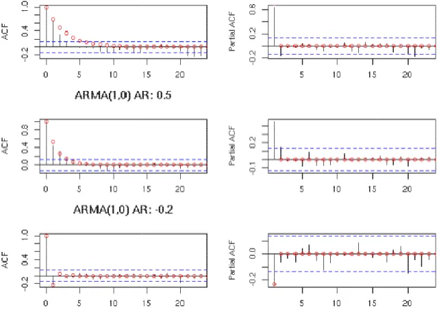
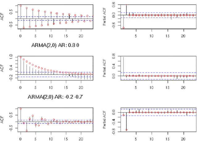
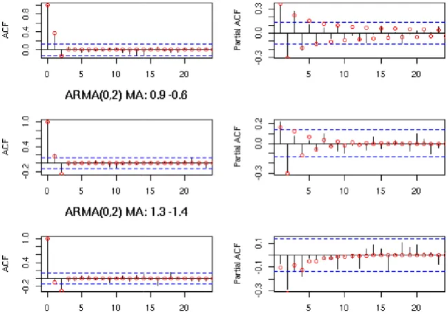
Figure 3.1: Linear Regression Graph: ACF and PACF for an AR(1) process … 46 Figure 3.2: Linear Regression Graph: ACF and PACF for an AR(2) process … 47 Figure 3.3: Linear Regression Graph: ACF and PACF for a MA(1) process … 47
Figure 3.4: Linear Regression Graph: ACF and PACF for a MA(2) process … 66
1.0 Introduction
1.1 Background
Determination of exchange rates was once fairly simple. During the years of the Bretton Woods System (a system put in place in 1944 when the leaders of allied nations met at Bretton Woods, NH to set up a stable economic structure out of the chaos of World War II), there were long periods of exchange rate stability. Despite the inherent problems, pegged systems lend a degree of confidence to currency price predictions. There were major readjustments to the system if a currency became too far out of line with economics, but there were few surprises because adjustments could be anticipated well in advance. This is no longer the case.
Current practices rely on exchange rate forecasts as a cornerstone of most, if not all, international business and banking decisions. Speculations based on exchange rate forecasts provide the opportunity to create sizeable profits for businesses and banks. The constant movement of rates in the foreign exchange market, combined with the rapid internationalization of business, has resulted in the demand for forecasting methods.
In general, forecasting requires the presumption of a set of relationships among variables. In other words, economic forecasting requires models. Forecasting techniques are based on formal models and may rely on an assumed sequence of casual relationships (e.g., simulation models), or on the data-based development of statistical relationships
between the variable of interest and past values of the same series (intrinsic models),
and/or past values of various exogenous variables (extrinsic models).1
One feature common to both exploratory and causal and extrinsic and intrinsic statistical models is that their predictive ability depends on the assumption that
relationships established in the past will continue reasonably unchanged into the future. It makes little difference whether the nature of this relationship is specified in terms of a logical or theoretical framework, or a statistical dependence. The stability of the
forecasting model is not the only condition necessary for profitable forecasting. A more fundamental condition is that the actions of other forecasters do not wipe out any possible profit from successful prediction. Recent developments in time series theory have led to the frequent use of methods that forecast by fitting some functional relation to the historical values of the series and extrapolating them into the future.
The international monetary environment in which the exchange rate forecasts are made has passed through several transitions. The most common transition is that national monetary authorities have pledged to maintain exchange rates within small margins around a target rate or a “par value.” This value could be changed whenever the balance of payments of a country moves in disequilibrium and when it becomes clear that various alternative policies are ineffective. Forecasting procedures developed in this
environment consist of a three-step process: the examination of the balance of payments and other trends one derives from pressure on a currency; the indication from the level of central bank foreign exchange reserves (including borrowing facilities) of the point in
1
Ian H. Giddy and Gunter Dufey, "The Random Behavior of Flexible Exchange Rates: Implications for Forecasting." Journal of International Business Studies, 1 (1975): 1-32.
time when a situation becomes critical; and the crucial prediction of which one of the rather limited policy options economic decision-makers resort to in times of crisis.
1.2 Problem Statement and Purpose of the Thesis
World currencies are being traded everyday against one another to the tune of trillions of dollars per day. Through this trading each currency is pegged and measured against the other by an exchange rate. An exchange rate is the price of one currency expressed in terms of another currency. The question that arises is: what causes exchange rates to change, and how does one predict future value?
Time series analysis involves both model identification and parameter estimation. Most analyses would agree the identification problem is more difficult. Once the
functional form of a model is specified, estimating the model parameters is usually straightforward. To identify a model that best represents a time series, it is necessary to be clear about the purpose of the model. Is the model’s chief objective to explain the nature of the system generating the series? Or, is the model to be judged on its ability to predict future values of the time series? Therefore, to arrive at a model that represents only the main features of the series, a selection criterion, which balances model, fit, and
model complexity, must be used.2
The purpose of this thesis is to seek answers to different questions regarding the forecasting of foreign exchange rates. Exchange rate movement is regularly monitored by central banks for macroeconomic analysis and market surveillance purposes. Results in the literature show exchange rate models perform poorly in out-of-sample prediction
2
Eily Murphee and Anne Koehler, “A comparison of the Akaike and Schwarz Criteria for Selecting Model Order.” Applied Statistic, 37 (1988): 187-195.
analysis, even though some models have good in-sample analysis. The results were found using methods including moving average, exponential smoothing, random walk, and Box-Jenkins transfer function. The questions that I ask are: how accurate are these models when compared to a random prediction of future exchange rates, and what variables, if any, allow for the most accurate prediction? I am motivated to research this issue because I currently work in the insurance business and am interested in actuarial science.
This thesis is to research a variety of foreign exchange forecasting models and gather data for several different countries and variables in order to compare the future predictions to a random walk model. There are several objectives I will pursue to determine if this thesis is valid. One objective is to define the specific formulas used for each model, including which variable each model uses. Another objective is to run tests of all the models, variables, and data, and compare the viability of the results. A number of questions will arise and will be investigated.
The outcome of this course is my written statement. My anticipation of this thesis is that foreign exchange rate forecast models do not outperform a random walk model when predicting future rates. The evaluation of this course will be the assessment of my thesis and oral defense by my thesis committee.
1.3 Significance of the Thesis
International forecasts are usually settled in the near future. Exchange rate forecasts are necessary to evaluate the foreign denominated cash flows involved in international transactions. Thus, exchange rate forecasting is very important to evaluate the benefits and risks attached to the international business environment.
A wide variety of forecasting techniques and models claim that they are able to help predict future values of exchange rates. There is a need to investigate and evaluate these forecasting claims and compare the results accordingly.
This thesis provides comparative results that are important for forecast model selection used in predicting and trading foreign exchange rates. The results of this thesis will provide a foundation as to whether there is a clear-cut model that should be used in predicting foreign exchange rates.
The first question that arises is: are there different methods used in order to forecast different currencies? There are different methods of forecasting exchange rates. One approach may consider various factors specific to long-term cycle rise. For instance, data for a certain country would be looked at based on productivity indices, inflation, unemployment rate, trade balance, and more. A different approach focuses on the current and past real value of the exchange rate. Forecasting can be based on the investor, so changes in rate can be determined and patterns charted. There can be any number of methods used to attempt to predict the trend of the exchange rate and information such as political instability, natural disasters and speculation.
Currency speculation involves buying, selling and holding currencies in order to make a profit from favorable fluctuations in exchange rates. It involves a high degree of
risk since predicting what events will influence exchange rates during a specific period of time, as well as the magnitude of the influence, is very difficult. Currency speculation can have serious consequences on a national currency and accordingly on a country's economy. While a major benefit of speculation is an increase in liquidity (more units of currency being used in transactions rather than reserves), speculation can also devalue or inflate a currency to the point at which a country’s stock market and overall economy starts to follow suit. Heavy trading in a currency creates “artificial demand” and can increase the prices of goods beyond an inflation-adjusted level.
The second question that arises is: what are the macro variables that should be used for forecasting variables? Information plays an important role in regarding the potential return on foreign exchange trading. The general view about exchange rates is if the exchange rate of a country is properly valued, it does not substantially affect the macroeconomic variables and, therefore, the macroeconomic performance of that
country. Volatility in exchange rate of a country can affect the investment in that country adversely. It creates an uncertain environment for investment in that country and requires that the country’s resources be reallocated among various sectors of the country’s
economy.
One variable that plays a role in the movement of the exchange rate is foreign direct investment. The role of foreign direct investment for the growth of developing countries is very important. Foreign investors are motivated to invest in a host country if the prospects of earning long-term profits by contributing towards the country’s
capital formation in developing countries, but it is also a source of transfer of technological and innovative skills from developed to developing countries.
Inflation can also affect the fluctuation of an exchange rate. Inflation affects the value of goods and services because purchasing power parity is a fundamental
determinant of exchange rates. Inflation in one country translates into a rise in the price of goods and services in that country, whereas the value of products in other countries remains unchanged where inflation is subdued. The result of this discrepancy is that the currency of the country experiencing inflation plummets against those other currencies that do not, resulting in a devaluation of their currency.
An example of variables affecting the foreign exchange rate of a local currency can be seen in gross domestic product. If a country imports more goods and services than it exports, then the result is a current account deficit. That country must finance that current account deficit, either by international borrowing or by selling more capital assets than it buys internationally. Conversely, when the country exports more than it imports, its trading partners must finance their current account deficits, either by borrowing or by selling more capital assets than they purchased, both affecting the rate.
Another question now arises. Is forecasting feasible? In many ways, there is no conflict between fundamental and technical analysis. The decisions that result from economic or policy changes are far reaching; these actions may cause a long-term change in the direction of prices and may not be reflected immediately. Actions based on long-term forecasts may involve considerable risk. Integrated with a technical method of known risk, which determines price trends over shorter intervals, investors and researchers have gained practical solutions to their forecasting problems.
A fundamental study may be a composite of supply and demand elements such as statistical reports, expected use, political ramifications, labor influence, price support programs, and industrial development. The result of a fundamental analysis is a forecast. Technical analysis is a study of patterns and movements. Its elements are normally limited to price, volume, and open interest. It is considered to be the study of the market itself. The results of technical analysis may be a short- or long-term forecast based on recurring patterns; however, technical methods often limit their goals to the statement that prices are moving either up or down. One advantage of technical analysis is it is completely self-contained. The accuracy of the data is certain.
To successfully forecast, one must act on news that has not yet been printed and anticipate changes. One must recognize recurring patterns in price movement and determine the most likely results of such patterns. One must also determine the trend of the market by isolating the basic direction of data over a selected time interval.
Forecasts are limited by the data used in the analysis. This raises the question: what data should be used? There is a multitude of statistical data that might be used other than the data related to a specific inquiry. Some of this data is easily included such as prices, but other data may add to a more certain forecast; however, the data may not be that readily available. The time frame of the data impacts both the type of forecast as well as the nature of the forecast. For example, if using only weekly data, there is so much emphasis on the trend that your forecast is already pre-determined. A shorter time may guarantee a faster response to changes, but it does not assure better results.
When sampling is used to obtain data, it is common to divide entire subsets of data into discrete parts and attempt a representative sampling of each portion. These
samples are then weighted to reflect the perceived impact of each part on the whole. Such a weighting will magnify or reduce the errors in each of the discrete sections. The result of such weighting may cause an error in bias. Even large numbers within a sample cannot overcome intentional bias introduced by weighting one or more parts.
Technical analysis is based on a perfect set of data. Each price that is recorded is exact and reflects the netting out of all information at that moment. Most other statistical data, although appearing to be very specific, are normally an average value, which can represent a broad range of numbers, all of them either large or small. When an average is used, it is necessary to collect enough data to make that average accurate. When using small, incomplete, or representative sets of data, the approximate error, or accuracy of the sample, should be known. A critical element of forecasting is the recognition that there exists a pattern in the time series data. Forecasting a trend or cycle requires a
methodology different from that of forecasting seasonal differences. A time series is nothing more than observed successive values of a variable or variables over regular intervals of time.
There are four basic components that make up time series data that can influence our forecast of future outcomes:
Secular trend (
T
)Seasonal variation (S)
Cyclical variations (C)
Random or irregular variation ( )3
3
J.K. Sharma, Business Statistics (New Delhi, India: Dorling Kindersley, 2007), 543.
The time series model that is generally used is a multiplicative model that shows
the relationship between each component and the original data of a time series (
Y
) as:Y=T∗S∗C∗I
Secular trend is the long-term growth movement of a time series. The trend may be upward, downward, or steady. Seasonal variation refers to repetitive fluctuations that occur within a period of one year. Cyclical variations are wave-like movements that are observable over extended periods of time. Random variation refers to variation in a time series that is not accounted for by trend, seasonal, or cyclical variations. Because of its unsystematic nature, the random or irregular variation is erratic with no discernible pattern.
The final question that needs to be answered is: do any of the techniques
outperform the random walk model? Some methods of analyzing data are more complex than others. All good forecasting methods begin with a sound premise. One must first know what he or she is trying to extract from the data before selecting a technique. The choice of methods depends on the specifics of the situation as well as the formal
statistical criteria that guide model selection within certain approaches. The choice of selecting a technique depends on the objectives of that forecast.
Forecasting methodologies fall into three categories: quantitative models, qualitative models, and technological approaches. Quantitative models, also known as statistical models, are objective approaches to forecasting. They dominate the field as they provide a systematic series of steps that can be replicated and applied to a variety of conditions. The qualitative methods of forecasting are called non-statistical or judgmental approaches to making forecasts. These approaches depend heavily on expert opinion and
the forecaster’s judgment. The qualitative
are scarce. The techniques used in the technological approach combine the quantitative and qualitative approaches so that a long
model are to respond to technologic to make a forecast. 4 Figure 1
Figure 1-1
4 Perry J. Kaufman, Trading Systems and Methods
the forecaster’s judgment. The qualitative approaches are adopted when historical data are scarce. The techniques used in the technological approach combine the quantitative and qualitative approaches so that a long-term forecast is made. The objectives of the model are to respond to technological, societal, political, and economic changes in order
Figure 1-1 shows the process of model selection.
Trading Systems and Methods (New York: John Wiley & Sons, 1998), 1
approaches are adopted when historical data are scarce. The techniques used in the technological approach combine the quantitative
term forecast is made. The objectives of the al, societal, political, and economic changes in order
1.4 The Path of Query
Regression analysis is a way of measuring the relationship between two or more sets of data and involves statistical measurements that determine the type of relationship that exists between the data studied. Regression analysis is often applied separately to the basic components of a time series, that is, the trend, seasonal or secular, and cyclic elements. These three factors are present in all price data. The part of the data that cannot be explained by these three elements is considered random or unaccountable.
Trends are the basis of many trading systems. Long-term trends can be related to economic factors such as inflation or shifts in the U.S. dollar due to the balance of trade or changing interest rates. The reasons for the existence of short-term trends are not always clear since trends that exist over a period of a few days cannot always be related
to economic factors but may be strictly behavioral. 5
The random element of price movement is a composite of everything
unexplained. There is a special relationship in the way price moves over various time intervals, the way price reacts to periodic reports, and the way prices fluctuate due to the time of the year. Most trading strategies use one price per day, usually the closing price, but some methods will average the high, low, and closing prices. Economic analysis operates on weekly or monthly average data but may use a single price for convenience. Two reasons for the infrequent data are the availability of most major statistics on supply and demand and the intrinsic long-term perspective of the analysis. The use of less frequent data will cause a smoothing effect. The highest and lowest prices will no longer
5
appear, and the data will seem more stable. Even when using daily data, the intraday
highs and lows have been eliminated, and the closing prices show less erratic movement.6
A regression analysis, which identifies the trend over a specific time period, will not be influenced by cyclic patterns or short-term trends that are the same length as the time interval used in the analysis. The time interval used in the regression analysis is selected to be long (or multiples of other cycles) if the impact of short-term patterns is to be reduced. To emphasize the movement caused by other phenomena, the time interval should be less than one-half of that period. In this way, a trend technique or forecasting
model may be used to identify a seasonal or cyclic element. 7
Having discussed the research problem, purpose and need for evaluating, and selecting forecasting models, we now describe and summarize related research conducted in this field by previous experts and economists. This is followed by a discussion of the methodology that is used along with conclusions and recommendations for future research and development.
Data gathered for this project was collected from the Federal Reserve Bank of St. Louis website. There were three variables used for four different countries. The
countries used were Japan, Canada, Great Britain, and the United States. All variables used are for the time period of January 1980 to October 2010, based on a quarterly frequency. The aggregation method used for each variable is an average.
The first variable is foreign exchange rates. The data uses an average of the daily figures based on buying rates in New York City and is based upon one denomination of local currency compared to one U.S. Dollar.
6
Cheol S. Eun and Bruce G. Resnick, International Financial Management (New Delhi: McGraw Hill, 2008), 59-73.
7 Ibid.,
The next variable used is gross domestic product (GDP). The GDP data for Japan is seasonally adjusted based on billions of Japanese YEN. Canadian GDP is seasonally adjusted data based upon millions of Canadian Dollars. GDP in Great Britain is also seasonally adjusted based upon millions of British Pounds.
The third variable used is CPI, or Consumer Price Index. This data is not seasonally adjusted and is denoted as a percentage. These variables are selected for this study after consulting foreign exchange traders at Citibank. Although several other variables can and are used, these are the three that are consistent among the several trading desks.
1.5 Limitations
A forecast represents an expectation about a future value or values of a variable. The expectation is constructed using an information set selected by the forecaster. The exchange rate depends on fundamentals such as relative national money supplies, real incomes, short-term interest rates, expected inflation differentials, and cumulated trade balances. These fundamentals are currently used by the head traders of foreign exchange currencies at Citibank.
There are several limitations that can be identified in evaluating forecasting performance. One limitation in time series forecasting is that the data may or may not be adjusted for seasonality, which is used to balance data fluctuation over a period of time. This can also be referred to as stationarity, in which data is transformed to include or exclude seasonal trends.
There are also factors that lead to long-run real exchange rates that may not be found in historical data. The factors can range from economic crisis to natural disasters. Examples are war, earthquakes, political turmoil, oil prices, and global trade patterns.
The topic of economic forecasting is vast and many models have been presented over the years. There is no way to determine which forecasting model is the best fit due to limitations and the inability to predict future occurrences. The purpose of this thesis is to answer the four main questions that arose during research. Are there different methods used in order to forecast different currencies? What are the macro variables that should be used to forecast currencies? Is forecasting feasible? Do any of the techniques outperform the random walk model?
2.0 Review of Literature
In this study we look to use exchange rate as a dependent variable. The need for the intermediate monetary target variable arises because monetary instruments (e.g., the bank rate, cash reserve requirements, open market operations), and the ultimate goal of monetary policy (e.g., a higher rate of economic growth, price stability, a surplus in the balance of payments) do not have a direct relationship. In order to determine if exchange rates influence GDP and interest rates, we most know the link between them.
Exchange rate fluctuations play a key role in determining economic policy. These fluctuations have repercussions on economic performances. It is essentially the
dependence with respect to imports and specialization in exports that account for exchange rate fluctuations on the economic performances of countries. In order to
stabilize the economy during these fluctuations, government may increase or decrease money supplies, which, in turn, can weaken or strengthen the price of the exchange rate.
In fundamental models of exchange rate, macroeconomic variables such as interest rates, money supplies, gross domestic products, trade account balances, and commodity prices have long been perceived as the determinants of the equilibrium exchange rate. The foreign exchange rate in fundamental models is classified as a highly liquid market where all information is public, and traders in the market share the same
expectations with no information advantage over the other.8
2.1 Exchange Rate Systems
Confidence in a currency is the greatest determinant of an exchange rate.
Decisions based on expected future developments may affect the currency. An exchange of currency can be based on one of four main types of exchange rate systems:
Fully fixed exchange rates Semi-fixed exchange rates Free-floating exchange rates
Managed floating exchange rates 9
The Federal Reserve Bank of New York carries out foreign exchange-related activities on behalf of the Federal Reserve System and the U.S. Treasury. In this
capacity, the bank monitors and analyzes global financial market developments, manages
8
Andrew W. Mullinex and Victor Murnide, Handbook of International Banking (London: Edward Elgar Publishing Limited, 2003), 350-358.
9 The Federal Reserve Board. "FRB: Speech, Bernanke--International Monetary Reform and Capital
Freedom--October 14, 2004." http://www.federalreserve.gov/boarddocs/speeches/2004/20041014/
the U.S. foreign currency reserves, and from time to time intervenes in the foreign exchange market.
The U.S. Treasury has the overall responsibility for managing the U.S.
government’s foreign currency holdings. It works closely with the Federal Reserve to regulate the dollar’s position in the forex markets. If the Treasury feels there is a need to weaken or strengthen the dollar, it instructs the Federal Reserve Bank of New York to intervene in the forex market as the Treasury’s agent. The Federal Reserve Bank of New York buys dollars and sells foreign currency to support the value of the dollar. The bank also sells dollars and buys foreign currency to try to exert downward pressure on the price of the dollar. 10
The transactions in the intervention are small compared to the total volume of trading in the forex market, and these actions do not shift the balance of supply and demand immediately. Instead, intervention is used as a device to signal a desired
exchange rate movement and affect the behavior of investors in the forex market. Central banks in other countries have similar concerns about their currencies and sometimes intervene in the forex market as well. Usually, intervention operations are undertaken in coordination with other central banks. Some countries have special arrangements with other countries to help them keep their currencies stable. Many less developed countries have their currencies pegged to other currencies so that their value rises and falls
simultaneously with the stronger currency. 11
In a fully fixed exchange rate system, the government (or the central bank acting on its behalf) intervenes in the currency market in order to keep the exchange rate close
10
The Federal Reserve Board. "FRB: Speech, Bernanke--International Monetary Reform and Capital Freedom--October 14, 2004”.
11
to a fixed target. It is committed to a single fixed exchange rate and does not allow major fluctuations from this central rate. In a semi-fixed exchange rate system, currency can move inside permitted ranges of fluctuation. The exchange rate is the dominant target of economic policy making. Interest rates are set to meet the target, and the exchange rate is given a specific target. This is the major difference between fully and semi-fixed
exchanges rates. However, the semi-fixed holds most of the same characteristics as the fully fixed exchange rate. 12
A floating exchange rate system is a monetary system in which exchange rates are allowed to move due to market forces without interventions of national governments. With floating exchange rates, changes in market demand and supply cause a currency to change a value. Pure free-floating exchange rates are rare. Most governments at one time or another seek to manage the value of their currency through changes in interest. In a free-floating exchange rate system, the value of the currency is determined solely by market supply and demand forces in the foreign exchange market. Trade flows and
capital flows are the main factors affecting the exchange rates and other controls.13
2.2 Exchange Rate Variables
In looking domestically at the United States, the current account deficit is conceptually equal to the gap between domestic investment and domestic saving as
12 The Federal Reserve Board. "FRB: Speech, Bernanke--International Monetary Reform and Capital
Freedom--October 14, 2004”.
matter of international account, which can be seen in the national income identity. The
following graph shows the 2012 U.S. trade deficit when compared to China. 14
2012: U.S. trade in goods with China
NOTE: All figures are in millions of U.S. dollars on a nominal basis, not seasonally adjusted unless otherwise specified.Details may not equal totals due to rounding.
Month Exports Imports Balance
January 2012 8,372.0 34,394.6 -26,022.6 February 2012 8,760.7 28,124.7 -19,363.9 March 2012 9,829.7 31,501.8 -21,672.0 April 2012 8,456.5 33,011.0 -24,554.5 May 2012 8,898.6 34,942.0 -26,043.4 June 2012 8,518.7 35,919.8 -27,401.2 July 2012 8,554.1 37,929.9 -29,375.8 August 2012 8,609.2 37,297.3 -28,688.1 September 2012 8,790.9 37,849.9 -29,059.0 October 2012 10,823.3 40,289.5 -29,466.2 November 2012 10,594.4 39,548.2 -28,953.8 December 2012 10,382.0 34,835.0 -24,453.0 TOTAL 2012 110,590.1 425,643.6 -315,053.5
When investments in the United States are higher than domestic saving,
foreigners make up the difference, and the United States has a current account deficit. In contrast, if savings exceed investment in a country, then that country has a current account surplus and its people invest abroad. The growth of the U.S. current account deficit for more than a decade has been linked to high levels of domestic U.S. capital formation compared to domestic U.S. saving. Perceived high rates of return on U.S. assets (based on sustained strong productivity growth relative to the rest of the world)
14
The United States Census Bureau. "2012: U.S. trade in goods with China.”
show U.S. economic performance and the attractiveness of the U.S. investment climate, attracting foreign investment. Sustained external demand for the United States assets has both supported the dollar in the foreign exchange markets over the years and allowed the United States to achieve levels of capital formation that would have otherwise not been possible. Robust growth in investment is critical to the non-inflationary growth of
production and employment. 15
For a country to be involved in international trade, finance, and investment, it is necessary to have access to foreign currencies of other countries. The sale and purchase of foreign currencies take place in the foreign exchange markets. This market allows for the movement of large volumes of funds (about three trillion dollars per year) for
investment purposes around the world. Any changes in exchange rates are important because of the effect they have on the prices we pay for imports, the prices we receive for our exports, and the amount of money flowing into and out of the economy.
For example, if the volume of the U.S. dollar appreciates (increases in value), exports become more attractive and overseas customers have to find more U.S. dollars to buy the same volume of exports. If the U.S. dollar depreciates (decreases in value), then U.S. exports become cheaper, and imports become more attractive. U.S. exports are now more competitive in global markets because of the depreciation of the U.S. dollar. Currently, overseas buyers of U.S. products have to find fewer U.S. dollars to buy the same value of exports. Decreasing import prices can decrease production costs and inflation rates in any domestic economy.
15
The Federal Reserve Board. "FRB: Speech, Meyer -- The Future of Money and of Monetary Policy."
There are several factors that affect the demand for U.S. dollars. The first factor to look at is the demand for U.S. exports. When overseas consumers buy U.S. goods and services, they need to convert their currency into U.S. dollars to pay for the exports. Therefore, any increase in the demand for U.S. exports should increase the value of the dollar.
Changes in world economic conditions and international competitiveness will affect the demand for the U.S. dollar. High levels of world economic growth can increase the demand for goods and services and the demand for the U.S. dollar. To be competitive in the global market, the United States’ goods and services must be as cheap as its international competitors. If U.S. inflation rates and costs are relatively higher than its overseas competitors, then the goods and services will be more expensive. High U.S. inflation rates help cause a loss of export markets, reduce the demand for the dollar, and force a depreciation of the dollar. However, lower rates of inflation typically increase the
demand for U.S. exports and appreciate the value of the dollar. 16
Capital inflow also affects the demand for U.S. dollars. Foreign investors wishing to invest in the United States must also exchange their own currency for dollars. A number of factors may influence the investment decision. If interest rates are relatively higher than overseas interest rates, this will increase the capital inflow and the demand for U.S. dollars. The expectation of higher levels of domestic growth will influence the size of capital inflow and increase the demand for dollars, causing a currency
appreciation. A decline in the level of capital inflow, however, may cause a fall in the demand for dollars, resulting in currency depreciation.
16
There are also several factors that affect the supply of U.S. dollars. Demand for imports plays a significant role. Just as foreigners must pay for exports with U.S. dollars, we must pay overseas producers foreign currency for imported goods. If the dollar demand for imported goods and services increases, so does the supply of dollars. The increase in the supply of U.S. dollars puts downward pressure on the value of the dollar.
An increase in capital outflow can occur as a result of higher interest repayments on overseas loans (net income transfers) or increased demand for foreign assets. This means that investors need to sell U.S. dollars (increasing the supply) in the foreign exchange market to obtain other countries’ currencies. The increase in the supply of dollars could cause a decrease (depreciation) in the value of the U.S. dollar. The level of domestic interest rates and investor confidences in the U.S. dollar also influence the supply. If there are high rates of inflation in the United States, imported goods and services would be cheaper relative to domestically produced products. If speculators lose confidence in the economy and feel that future values of the U.S. dollar will be lower than present levels, a depreciation of the exchange rate can occur. This happens because when speculators sell U.S. dollars to avoid future losses, the supply of dollars increases, putting downward pressure on the exchange rate.
How does this information tie directly into the U.S. economy? The United States budget currently has a deficit or current account deficit. There is a process of adjustment to current account deficit. The possible causes of an emerging or growing current
account deficit are the same issues that cause depreciation as discussed earlier. Three of the most prominent causes are: domestic incomes increasing at a faster pace than foreign
incomes; domestic inflation at a faster pace than foreign inflation rates; and domestic interest rates that are lower than foreign interest rates.
A growing deficit is likely to increase the supply of domestic money to the foreign exchange market. Assuming that the demand for domestic money has not changed, the resulting excess supply will likely induce depreciation of the domestic currency on the foreign exchange market. The depreciation of the domestic currency makes the nation’s exportable goods look cheaper to foreigners and imports from abroad appear more expensive to citizens, thereby alleviating the current deficit. How foreign exchange market transactions affect the domestic supply of a nation depends upon the identities of the purchasers and sellers of the exchange. With a current deficit, one source of the increased supply of domestic currency to the forex market is foreigners who have acquired the domestic currency as export earnings, incomes from investors in the nation, or transfers from citizens or government of the nation. If foreigners supply quantities of the domestic currency to other foreigners through the forex market, the relevant domestic money supply (that which motivates the behavior of citizens of the nation) does not change.
Another source of increased supply of domestic currency to the forex market is the efforts by citizens of the nation to convert quantities of domestic currency into foreign currencies in order to purchase imports from foreign sources, invest overseas, or make transfers to foreigners. To the extent that foreign interests acquire money balances denominated in units of the domestic currency from citizens of the nation, the nation’s relevant domestic money supply decreases. Assuming that the domestic demand for money does not change, the domestic money supply decrease may result in falling
domestic prices, rising domestic interest rates, and decreasing employment. The falling domestic prices of goods tend to increase the volume of exports and reduce the volume of imports. The rising domestic interest rates tend to decrease the volume of investment by citizens in other countries and increase the volume of investment by foreigners in the nation. The decreasing domestic employment decreases income in the nation and, thus, curbs imports.
One view is that the burden of adjustment borne by domestic prices, interest rates, and employment is lessened by the currency depreciation. Another view is that these three phenomena supplement the depreciation of the domestic currency in alleviating the current deficit. However, if the depreciation of the domestic currency is prevented by government authorities that are resolved to “defend the currency” from further weakening or depreciation, the burden of adjustment to the deficit will descend upon domestic
prices, interest rates, and employment. 17
Some of the domestic money, which is supplied to the forex market, may be acquired by citizens of the nation who may wish to convert foreign currency denominated export earnings, investment income, or gifts from foreigners into domestic currency for repatriation. Such currency transactions between citizens of the same nation do not affect the domestic money supply, even though they pass through the forex market. Such citizen-to-citizen forex market transactions may be large enough relative to the volume of transactions between citizens and foreigners that the reduction of the domestic money supply consequent upon a deficit will itself be diminished. Although the usual
presumption is that the domestic money supply decreases, the volume of citizen-to-citizen or foreigner-to-foreigner transactions in the domestic currency is large enough
17
that the money supply may be little affected by a deficit. In this case, the domestic macroeconomic adjustment will be minimal, and the correction of the imbalance will depend largely upon depreciation of the currency if the government will let it ensue.
The depressive macroeconomic effects of a decrease of the relevant domestic money supply in response to a deficit may motivate the government of the nation to attempt to neutralize the monetary contraction with offsetting purchases of bonds in the open market. If domestic macroeconomic contraction is prevented, the full burden of the adjustment of the deficit must fall upon exchange rate depreciation. If the government also resolves to prevent its currency from depreciating by intervening in the forex market to purchase quantities of the domestic currency, no mechanism of adjustment is allowed to function, and the current deficit may persist indefinitely. It may be inferred that a fixed exchange rate system is fundamentally incompatible with the exercise of modern
macroeconomic policy to stabilize the domestic economy. 18
2.3 Meese & Rogoff
The difficulty in predicting future exchange rates has been a longstanding issue in international economics. The forecasting experiment proposed by Richard Meese and Kenneth Rogoff is by what exchange rate models are judged. Meese and Rogoff examined the relationship between real exchange rates and real interest rates over the modern (post 1970) flexible rate period. They concluded that the exchange rate depends on fundamentals such as relative national money supplies, real incomes, short-term interest rates, expected inflation differentials, and cumulated trade balances. The
18
Robert Wade, Governing The Market: Economic Theory and the Role of Government in East Asian Industrialization (New Jersey: Princeton University Press, 1990), 159-168.
underlying assumption is that goods market prices adjust slowly in response to anticipated disturbances and to excess demand. Consequently, less than perfectly anticipated monetary disturbances can cause temporary deviations in the real exchange rate from its long-run equilibrium value. Meese and Rogoff used the following equation for forecasting exchange rates:
( ) ( − = Ε + + θ k k t k t t q q q
where Εt is the time expectations operator,
prevail at time t if all prices were fully flexible, and
parameter. In addition,
θ
is a function of the structural parameters of the model.However, additive disturbances (such as money market shocks) do not affect general, Εt (q
t+k) will not equal
shocks follow random walk processes. Meese & Rogoff challenged the long
determine currency values. They found that a random walk model was just as good at predicting exchange rates as models based on fundamentals. In short, their findings suggest economic fundamentals, like trade balances, money supply, national income, and other key variables, are of little use in forecasting exchange rates between countries with roughly similar inflation rates.
19
Kenneth Rogoff and Richard Meese, "Was it Real? The Exchange Rate Over the Modern Floating-Rate Period."
20
Ibid.
21
Ibid.
underlying assumption is that goods market prices adjust slowly in response to anticipated disturbances and to excess demand. Consequently, less than perfectly
disturbances can cause temporary deviations in the real exchange run equilibrium value. Meese and Rogoff used the following equation for forecasting exchange rates:
1 0 ), < < − θ k t q q tations operator, t
q is the real exchange rate that would
if all prices were fully flexible, and
θ
is the speed of adjustmentis a function of the structural parameters of the model. However, additive disturbances (such as money market shocks) do not affect
will not equal qt unless there are no real shocks or unless all real
shocks follow random walk processes.20
Meese & Rogoff challenged the long-held idea that economic fundamentals determine currency values. They found that a random walk model was just as good at
exchange rates as models based on fundamentals. In short, their findings suggest economic fundamentals, like trade balances, money supply, national income, and other key variables, are of little use in forecasting exchange rates between countries with
ghly similar inflation rates. 21
Kenneth Rogoff and Richard Meese, "Was it Real? The Exchange Rate-Interest Differential Relation Rate Period." The Journal of Finance, no. 43 (September 1998): 933 underlying assumption is that goods market prices adjust slowly in response to anticipated disturbances and to excess demand. Consequently, less than perfectly
disturbances can cause temporary deviations in the real exchange run equilibrium value. Meese and Rogoff used the following equation
is the real exchange rate that would is the speed of adjustment
is a function of the structural parameters of the model.19
However, additive disturbances (such as money market shocks) do not affect
θ
. Inunless there are no real shocks or unless all real
held idea that economic fundamentals determine currency values. They found that a random walk model was just as good at
exchange rates as models based on fundamentals. In short, their findings suggest economic fundamentals, like trade balances, money supply, national income, and other key variables, are of little use in forecasting exchange rates between countries with
Interest Differential Relation , no. 43 (September 1998): 933-948
2.4 Random Walk Model
It has been the position of many fundamental and economic analysis advocates that there is no sequential correlation between the direction of a price movement from one day to the next. Their position is that prices will seek a level that will balance the supply and demand factors, but that this level will be reached in an unpredictable manner as prices move in an irregular response to the latest available information or news release.
If the random walk theory is correct, many well-defined trading methods based on mathematics and pattern recognition will fail. The strongest argument against the
random movement supporters is price anticipation. One can argue that all participants (the market) know exactly where prices should move following the release of news.
Excluding anticipation, the apparent random movement of prices depends on both the time interval and the frequency of data used. When a long time span is used, from one to twenty years, and the data are averaged to increase the smoothing process, the trending characteristics will change, along with seasonal and cyclic variations. Technical methods such as moving averages are often used to isolate these price characteristics. The averaging of data into quarterly prices will smooth out the irregular daily movements and results in noticeably positive correlations between successive prices. The use of daily data over a long-term interval introduces noise and obscures uniform patterns.
In the long run, most future prices find a level of equilibrium and, over some time period, show characteristics of mean reverting (returning to a local average price);
however, short-term price movement can be very different from a random series of numbers. It often contains two unique properties: exceptionally long runs of price in a single direction, and asymmetry, the unequal size of moves in different directions.
Although the long-term trends are not of great interest to future traders, short-tern price movements, which are cause by anticipation rather than actual events, and extreme volatility, prices that are seen far from value, countertrend systems that rely on mean reversion, and those that attempt to capture trends of less duration, have been
successful.22
Meese & Rogoff considered six univariate time series models involving a variety of pre-filtering techniques and lag length selection criteria, a random walk with drift parameter, and an unconstrained vector auto regression; none could out-predict the
random walk model: , where is white noise with mean zero and constant
variance.
The six time series models used were the following: (1) an unconstrained auto
regression (AR) in which the longest lag considered (M) is set to equal (n/log, n), where n
is the sample size; (2) AR in which lag lengths are determined by Schwarz’s criterion; (3) AR in which lag lengths are determined by Akaike’s criterion; (4) long AR estimated by using observations that are arbitrarily weighed by powers of 0.95; (5) the
Wiener-Kolmogorov prediction formula; (6) AR estimated by minimizing the sum of the absolute values of errors. The pre-filtering techniques involve differencing, de-seasonalizing, and removing time trends.
The following three formulas define the random-walk model:
(1a) Sˆt+i= St+i−1 i = 1,2,…..15
22
Kaufman, Trading Systems and Methods, 37. t t
t s a
s = +
(1b) Sˆt+i = St i = 1,2,…..15
(1c) Sˆt+i = iuˆ+ St i = 1,2,…..15
where is the simple arithmetic mean of the changes in the values of in the estimation
period.23
2.5 Akaike and Schwarz Criteria
As stated earlier, time series analysis involves both model identification and parameter estimation, and a selection criterion that balances model, fit, and model complexity must be used to arrive at a model. The Akaike information criterion (AIC) (Akaike, 1974) and Schwarz information criterion (SIC) (Schwarz, 1978) are two
objective measures of a model’s suitability, which take these considerations into account. They differ in terms of the penalty attached to increasing the model order.
Given observations Y(1)…..Y(n), define Mj (Y(1),…..Y(n)) to be the maximum
value of the likelihood for the jth model under consideration. The Akaike procedure is to
choose the model that minimizes
2 1, … . . 2,
where is the number of free parameters in the model. The Schwarz criterion is to
choose the model that minimizes
2 1, … . .
23
Murphree and Koehler, "A comparison of the Akaike and Schwarz Criteria for Selecting Model Order," 187-195.
Therefore, if n≥ 8, the Schwarz criterion will tend to favor models of lower dimension
than those chosen by the AIC.24
This criterion concluded that the AIC would frequently choose higher order models for empirical data. Also, in forecasts for series when the AIC and SIC models differ, there is evidence that neither criterion has a clear edge in identifying models having small prediction set errors. The findings of this study argue for using SUC rather than AIC to choose the order of ARIMA model.
2.6 Wiener-Kolmogorv Filter
The Wiener-Kolmogorov (WK) signal extraction filter, extended to handle nonstationary signal and noise, has minimum Mean Square Error (MSE) among filters that preserve the signal's initial values; however, the stochastic dynamics of the signal estimate typically differ substantially from that of the target. The use of such filters, although widespread, is observed to produce dips in the spectrum of the seasonal
adjustments of seasonal time series. These spectral troughs tend to correspond to negative autocorrelations at lags 12 and 24 in practice, a phenomenon that will be called "negative seasonality." So-called "square root" WK filters were introduced by Wecker in the case of stationary signal and noise to ensure that the signal estimate shared the same stochastic dynamics as the original signal, and, therefore, remove the problem of spectral dips.
This represents a different statistical philosophy: not only do we want to closely estimate a target quantity, but also we desire that the internal properties and dynamics of our estimate closely resemble those of the target. The MSE criterion ignores this aspect
of the signal extraction problem, whereas the square root WK filters account for this issue at the cost of accruing additional MSE. This paper provides empirical documentation of negative seasonality and provides matrix formulas for square root WK filters that are appropriate for finite samples of non-stationary time series. We apply these filters to
produce seasonal adjustments without inappropriate spectral troughs.25
2.7 Engel & West
A well-known stylized fact about nominal exchange rates among low-inflation advanced countries, particularly U.S. exchange rates, is that their logs are approximately random walks. Meese and Rogoff (1983) found that the structural models of the 1970s could not “beat” a random walk in explaining exchange-rate movements.
Why? One obvious explanation is that the macroeconomic variables that determine exchange rates themselves follow random walks. If the log of the nominal exchange rate is a linear function of forcing variables that are random walks, then it will inherit the random walk property. The problem with this explanation is that the
economic “fundamentals” proposed in the most popular of exchange rates do not, in fact, follow simple random walks.
One resolution to this problem is that there may be some other fundamentals, ones that have been proposed in some models but are not easily measurable or ones that have not yet been proposed at all, that are important in determining exchange rates. If these “unobserved” fundamentals follow random walks and dominate the variation in exchange
25 Tucker McElroy, "A Modified Model-based Seasonal Adjustment that Reduces Spectral Troughs and
Negative Seasonal Correlation." http://www.census.gov/srd/www/abstract/rrs2008-12.htm (accessed 2 March 2009).
rate changes, then exchange rates will nearly be random walks (even if the standard
“observed” fundamentals are not).26
Engel & West conclude that asset-market models, in which the exchange rate is expressed as a discontinued sum of the current and expected future values of the observed fundamentals, can account for a sizeable fraction of the variance when the discount factor is large. The Engel & West explanation for a random walk provides a rationale for a substantial fraction of the movement in exchange rates. But there is still a role for left-out forcing variables, perhaps money demand errors, a risk premium, mis-measurement of the fundamentals, or other variables implied by other theories or noise.
2.8 McCracken & Sapp
Since the breakdown of the Bretton Woods agreement, researchers have used a wide variety of structural models to try to predict exchange rate movements. Finding consistent evidence that these models outperform a random walk has proven elusive.
McCracken & Sapp use p values based on developed tests of forecast accuracy and
encompassing q values designed to mitigate multiple testing problems. Both p and q
values can be interpreted as measures of a statistics significance. For example, if a test
statistic has a p value of 5%, one would expect that among a random sample of pairs of
statistics and hypothesis from the same population as the statistic, that on average 5% of those hypothesis are null and have statistics that will reject. Conversely, if a statistic has
26
Kenneth D. West and Charles Engel, "Accounting for Exchange-Rate Variability in Present-Value Models When the Discount Factor Is near 1." The American Economic Review 94 (2004): 119-125.
a q value of 5%, you would expect on average that 5% of the statistics that reject actually
correspond to the null hypothesis. 27
The other statistic used to test for significance is MSE t statistic. These statistics provide evidence of short, medium, and long horizon predictability.
Out of 400 tests, there were 154 cases where the p values are less than 5%.
Similarly, of the 400 tests, 338 have q values less than 10%, while 210 have q values less
than 5%. The MSE t statistic shows that there are no significant changes in predictive
ability. All cases show values less than 10%.
Their findings suggest that detecting predictability in exchange rates using regressions can be strongly influenced by the choice of test statistics and the manner in which it is employed. The results also yielded evidence that structural exchange rate models do not exhibit an ability to predict exchange rates. Similar to other studies, the evidence is consistent with there being more short-term predictability in exchange rates, and the results are relatively insensitive to the choice of the model.
2.9 Zhang & Berardi
Artificial neural networks have been widely used as a promising alternative approach to time series forecasting. Neural networks are data-driven, self-adaptive nonlinear methods that do not require specific assumptions about the underlying model. Instead of fitting the data with a pre-specified model form, neural networks let the data itself serve as direct evidence to support the model’s estimation of the underlying generation process. The network ultimately selected may not be the true optimal model
27 Michael, W. McCracken and Stephen G. Sapp, "Evaluating the Predictability of Exchange Rates Using
Long-Horizon Regressions: Mind your p’s and q’s." Journal of Money, Credit and Banking, Vol. 37, No. 3 (June 2005): 473-494.
because of a large number of factors that could affect neural network training and model selection. These factors include network architecture, activation functions, training algorithm, and data normalization. Alternative data sampling from a stationary process can have a significant effect on individual model selection and prediction. This impact may be magnified if the process parameters evolve or shift over time.
For the methodology in this example, Zhang and Berardi use weekly exchange rate data. They combine neural networks trained with different initial random weights but with the same data. The neural network trained with different starting weights may be stuck with different minimums, each of which can have different forecasting
performances.
Results show that different approaches to forming ensembles for time series forecasting have quite different effects on forecasting results. Neural network ensembles created by simply varying the starting random weights are not as competent as the traditional random walk model. Therefore, this method of ensemble forecasting may not
be effective for forecasting exchange rates. 28
28 G.P. Zhang and V.L. Berardi, "Time Series Forecasting with Neural Network Ensembles: An application
for Exchange Rate Prediction." The Journal of the Operational Research Society, Vol. 52, 6 (June 2001): 652-664.
3.0 Methodology
Much of the probability theory of time series assumes that time series exhibit a constant mean and constant variance over time, a condition known as stationarity. Non-stationary components of time series can usually be removed to make the series
stationary. For example, one can take differences of a time series to remove trends or seasonal variations.
Forecasts are generated with forecasting equations consistent with the method used to estimate the model parameters. Thus, the estimation method specified controls the way the forecast produces results. The forecast procedure provides a way of forecasting one or more time series automatically. It does not enable you to identify models or test for model adequacy. This is why it is important to test and select the correct forecast model.
Statistical measures are helpful in determining the appropriate mathematical form for the forecast model (i.e. in deciding whether an autoregressive model, a moving
average model, or a mixed model should be used for a particular time series).29
Once one knows there is a fundamental relationship between data, based on the measuring of the properties of dependence and correlation, a formula can be found that expresses one price movement in terms of the other prices and data. The predictive qualities of these methods are best when applied to data that has been seen before, as in prices that are within the range of historic data. Forecasting reliability decreases sharply when values are based on extrapolation outside the previous occurrences. This
phenomenon will also be true of other trending methods. This is based on the movement
29
of historical data; when prices move to new levels, the result of the model will often deteriorate. The techniques most commonly used for evaluating the direction or tendency of prices, both within prior ranges and at new levels, are called autoregressive functions.
3.1 Estimation and Forecasting Methods
Time series forecasting methods are based on analysis of historical data. These methods support the assumption that past patterns in data can be used to forecast future data points. The following statistics are used to measure the forecast error:
1. Moving averages (simple moving average, weighted moving average): forecast is based on arithmetic average of a given number of past data points
2. Exponential smoothing (single exponential smoothing, double exponential smoothing): a type of weighted moving average that allows inclusion of trends, etc.
3. Mathematical models (trend lines, log-linear models, Fourier series, etc.): linear or non-linear models fitted to time-series data, usually by regression methods
4. Box-Jenkins method: autocorrelation methods used to identify underlying time series and to fit the "best" model
The components of the time series forecast model used contain the following components:
1.Average:the mean of the observations over time
2.Trend: a gradual increase or decrease in the average over time
3.Seasonal influence: predictable, short-term cycling behavior due to time of day, week,