USE OF MICRO TUBES AS AN ALTERNATIVE TO THE
DESIGN OF DRIP IRRIGATION SYSTEM
Muhammed Bhuiyan
School of Civil, Environmental and Chemical Engineering, RMIT University, Melbourne, VIC 3001, Australia,
Email: [email protected] Amir Keshtgar
School of Civil, Environmental and Chemical Engineering, RMIT University, Melbourne, VIC 3001, Australia,
Email: [email protected] Nira Jayasuriya
School of Civil, Environmental and Chemical Engineering, RMIT University, Melbourne, VIC 3001, Australia,
Email: [email protected]
Abstract
Clogging and emission non-uniformity have been the major obstacles in the development of drip irrigation. To obtain best emission uniformity (EU) the pressure regulators and pressure compensating emitters are in use since long back. As pressure compensating emitters tend to be more complex, we suggest the possibility of utilizing varying length small bore polyethylene tubes (2-4 mm) along the laterals to provide simpler passages. The lengths of these small bore microtubes are varied according to the varying heads along a lateral that required to be compensated to deliver equal discharges. As such, the computed set of varying length microtubes that are emitting equal flows at the end-lateral can be replicated (i.e., by taking the same set of lengths) to subsequent laterals of the manifold to function them as larger emitters to have similar characteristic head-discharge relationship. As because the same set of microtube lengths are replicated to other laterals at upstream increasing heads, the variation of flows through those laterals are restricted by limiting their number to have EU ≥ 90 percent threshold. For case studies with EU ≥ 90 percent threshold on flat-ground for a given set of microtube (2-4 mm) and lateral (10-14 mm) diameters, the exponents in the head-discharge relationship varied narrowly: 0.60-0.69 for larger head-discharges and 0.78-0.84 for smaller discharges. Variation of the corresponding microtube lengths can be around 0-85% longer than the given minimum length (min=1.25 m). When the required discharges and diameters of microtube,
lateral and manifold and some other ground conditions are given, the length of the microtubes, the heads, emission uniformity and the best subunit dimensions can be obtained using the algorithm developed.
1. Introduction
The main objective of drip irrigation system is to provide soil moisture to each plant, which is sufficient to meet its transpiration demand. The microtube, also called „spaghetti tube‟ can be used as pressure compensating emitters in drip irrigation system. Utilizing these tubes as an alternative to current drippers will reduce the risk of clogging and blockage. Uneven distribution of flows from the system is always a problem faced by the drip irrigation designers. In order to overcome all these problems the hydraulics of microtube emitters in drip irrigation system has been studied by many researchers, some of the notables are Bucks and Myers (1973), Wu and Gitlin (1973), Khatri et al. (1979), Bagarello et al. (1995), Bhatnagar and Srivastava (2003), Almeida et al. (2009), etc.
Experimental results by Watters and Kellers (1978) confirmed that friction factor, f of the Darcy-Weisbach equation to calculate the head losses for smooth small diameter pipes (4 to 12 mm) can be calculated by using Blasuis formula. Experiments carried by von Bernuth and Wilson (1989) on larger diameter pipes (14, 16 and 26 mm) and for Reynolds number less than 100,000 also showed that the Blasius equation is an accurate predictor of the Darcy-Weisbach friction factors. Khatri et al. (1979) worked with seven different diameter microtubes (0.8 to 4 mm) to measure minor head losses in the system. Computations were done for the separation of minor losses to produce coefficients for different flow conditions. They concluded that using Blasuis equation has a reasonable accuracy for a range of tubes in turbulent flow condition.
Vermeiren and Jobling (1980) used microtube as emitter with very small diameters (0.5 to 1.1 mm) which are susceptible to blockage. Bhuiyan et al. (1990) studied on intermediate diameter microtubes (2 to 3 mm) which are easily available in the market. In their work an algorithm was developed for one single lateral to simulate the set of microtube lengths and discharge (equal for every microtube) for a given range of head, microtube and lateral diameters and number of trees to be irrigated.
The relation between pressure head and discharge has been studied in Keller and Karmeli (1974a, b) to show that it follows a power-law for customary emitters. They also gave the principles for discharge (or emission) uniformity in the system. So, the aim of this paper is to extend the previous researches on the analysis of drip irrigation system to design one typical subunit using microtubes as emitters. A typical subunit would comprise one manifold to branch into several laterals and then each lateral supplies to microtubes at a regular interval to discharge water at the roots of the plants. In the system along with the microtubes, the laterals would also be considered as larger emitters in the body of the manifold. The analysis would show that regardless of inlet head, the discharge distribution along a lateral would be equal. However, among the laterals in the manifold the discharge would follow emission uniformity (EU) greater than 90 percent.
2. System components
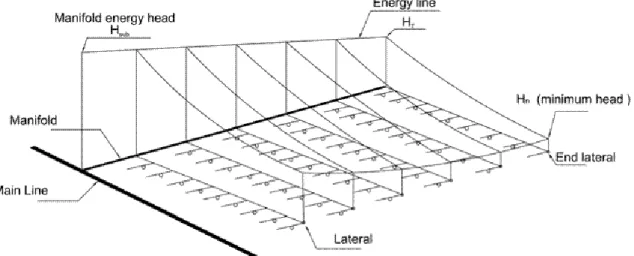
Figure 1 shows a typical subunit consisting of manifold, laterals and microtubes. Microtubes are emerging from the sides of the laterals as emitters. The energy grade line of the system is also shown
in the figure. The set of microtubes with varying lengths have been shown below in one side of the laterals.
a)
b)
Figure 1: Schematic layout of a typical drip irrigation subunit; a) subunit consist of manifold, laterals and microtubes, and b) varying length microtubes as emitters in one side of a lateral, details A and B show the installation methods for making coils (Keshtgar et al. 2012)
It will be demonstrated subsequently that to achieve equal discharges qo q1q2...qn for up (positive) and flat (zero) slopes, the microtube lengths would be o 12...(nmin). The microtube length n at the end of the lateral is taken as the minimum length, determined from realistic distances between crops and laterals. But for a down slope (negative) the location of the minimum length, min may be located anywhere in the sequence of n points along the laterals. The
equal discharges for all the microtubes in the lateral. As shown in Figure 1(b) the increased length of microtubes can be wrapped around a stick (detail A), or the lateral (detail B) to keep a constant distance between lateral and the plant. In this paper the term „coil‟ is used with a diameter of 3 cm (using detail A), which can be altered by the designer in other circumstances.
So with the given configuration in the subunit, the laterals at different points in the manifold will deliver increasingly more discharges due to increasing heads in their upstream inlets, whereas the microtubes in each of these laterals will deliver proportionately equal discharges by dividing those increasing discharges. Due to practical reason the scope of varying lateral lengths is limited to have equal flow rates through each lateral. So a characteristic head-discharge power-law relationship for the above end-lateral will be developed by regression analysis for the given set of discharges and its corresponding heads necessary as explained in the following section. This relationship may then be used to limit the widely increasing variation of discharges by maximising the number of laterals to be emerged from the manifold of the subunit in order to maintain the emission uniformity of the laterals above some given threshold value, say EU
90 percent. Here as the same set of microtube lengths and diameters are used in all the following laterals, these laterals also act as emitters with characteristic power-law relationship developed in any lateral (say, at the end-lateral) in the body of the manifold.3. Basic hydraulics
Darcy-Weisbach equation to calculate frictional head losses in pipes can be written in MKS units as
g v d f hf 2 2 (1)
For laminar flow the friction factor
f
can be written ase
R
f
64
(2)For turbulent flow with Reynolds number between 3000 and 100,000, Blasius equation which yields good approximation for computing friction factor
f
, can be written as25 . 0
32
.
0
eR
f
(3)where
R
e= Reynolds number,h
f = frictional head loss, and d= length and diameter of the pipes, g= acceleration due to gravity, andv
= velocity of flow. Equations (1-3) can be combined to obtain the equations for laminar (Equation 4) and turbulent (Equation 5) flows, respectively:4
32
.
1
d
q
h
f
(4) 75 . 4 75 . 1486
.
0
d
q
h
f
(5)where
h
f = friction head loss (m), q= discharge (litre/hr), d= diameter of the pipe (mm), = length of the pipe (m). Kinematic viscosity of water at 15˚C is taken as
= 1.14×10⁻⁶ m2/s.Velocity and other minor losses of the system can be written in general form as
g
v
k
h
2
2
(6)where k= head loss coefficient, which in three different minor loss coefficients are differentiated as: (i) ke= 1.2, to calculate entrance head loss assuming the entrance from lateral as a re-entrant one, (ii)
v
k = 1, to calculate velocity head, and (iii) kc= c1.3, to calculate coil head loss, where 1.3 has been extrapolated (for D/d≈ 12.0 and = 360˚, where D and d are the coil and pipe diameters and is the angle of bend subtended at the centre) from Ito‟s (1960) diagram on loss coefficient for smooth bends, c is the number of coils that can be computed from difference of two microtube lengths as
Dc n1n . Only whole number of coils is taken for the calculation of head losses. Thus, Equation (6) can be rearranged to accommodate the above three different minor losses as follows:
4 2
0077
.
0
d
q
h
e
(7) 4 20064
.
0
d
q
h
v
(8) 4 20083
.
0
d
q
m
h
c
(9)Energy grade line as shown in Figure 2 is related to head losses in one side of the lateral. Total head at the inlet of the microtube at point n can be calculated by summing all the head losses as follows:
n f
v
e h h n H
h ( ) (10)
Figure 2: Energy grade line and head losses in one side of the lateral (he= entrance loss, hv= velocity loss, hc= coil head loss, hf(n)= microtube friction head loss at n, and hfl(n)= lateral friction head loss between n and n1) (Keshtgar et al. 2012)
m Q 2 Q 1 Q
QjBy placing the microtube with minimum length at the point n, the balance of energy heads between two successive points, (n1) and n can be written as
S n h n h h h n h n h h he v f( 1) c( 1) e v f( ) fl( ) (11)
where S and are slope of lateral and distance between microtubes, respectively. Since the discharges are same in all the microtubes, entrance and velocity head losses are equal in all the microtubes, so Equation (11) can be written as
S n h n h n h n hf( 1) c( 1) f( ) fl( ) (12)
By substituting full expressions for each of the head balance terms there will be a total four equations for four combinations of laminar and turbulent conditions in lateral and microtubes as follows:
1. Flow regimes are laminar in both the microtube and lateral
S d nq d q d cq d q l m n m m n 4 4 4 2 4 1 0.0083 1.32 1.32 32 . 1 (13)
2. Flow regimes are laminar and turbulent in microtube and lateral, respectively
S d nq d q d cq d q l m n m m n 75 . 4 75 . 1 4 4 2 4 1 0.0083 1.32 0.486 32 . 1 (14)
3. Flow regimes are turbulent and laminar in microtube and lateral, respectively
S d nq d q d cq d q l m n m m n 4 75 . 4 75 . 1 4 2 75 . 4 75 . 1 1 0.0083 0.486 1.32 486 . 0 (15)
4. Flow regimes are turbulent in both the microtube and lateral
S d nq d q d cq d q l m n m m n 75 . 4 75 . 1 75 . 4 75 . 1 4 2 75 . 4 75 . 1 1 0.0083 0.486 0.486 486 . 0 (16)
Therefore, when the discharge required in the trees, diameters of microtube and lateral, slope, distance between microtubes, number of microtubes and the minimum length of microtube (
min
n) are known, the only unknown
n1 can be calculated from the above equations.Proceeding in this way up to the inlet of the lateral, all the microtube lengths will be known for delivering equal discharges q. After summing all the head losses along the lateral, the total head at the entry of the lateral is equal to inlet head
H
T. So in the lateral under inlet headH
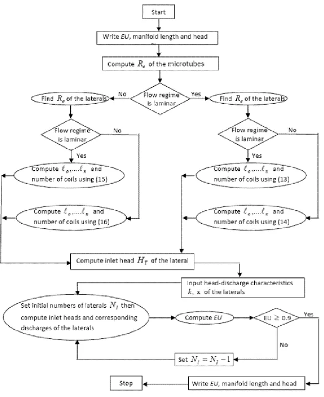
T, the total discharge entering would be Ql (n1)q.A computer program has been developed using the above algorithm. Figure 3 shows the flowchart of the program to compute microtube lengths, number of coils in each microtube and the head at the entry of the lateral HT. It also calculates the number of laterals that can be included in the manifold of a subunit to fulfil the condition of emission uniformity, EU90 percent. The inlet heads for the
successive laterals can be calculated using similar friction and minor losses in the manifold reaches up to the entry point of the manifold. This entry head of the manifold (Hsub) would be the operating pressure of the subunit that need to be provided for running the irrigation system.
4. Head-discharge relationship
Keller and Karmeli (1974) suggested a power-form flow equation for customary emitters as
x
kH
Q (17)
where Q= the emitter discharge (litre/hr), H= energy head at the emitter (m), k = the constant coefficient that characterizes each emitter, and x = the exponent that characterizes emitter flow regime.
By using the aforesaid equation, the emitter‟s head-discharge relationship can be generalized to laterals for designing them as emitters in the manifold line. To apply the concept, it is the same set of microtube lengths as calculated in the end-lateral are adapted to the rest of the laterals along the manifold. By taking a range of realistic discharges needed for the trees, the consequent heads are computed using Equations (13-16) in Section 3. These heads and discharges are plotted to obtain k
and x for the chosen lateral with high R2value for a feasible accuracy to consider laterals as emitters. For the given manifold size (dmd) and minimum operational head required at the inlet of the end-lateral, the discharge in the next lateral can be estimated by taking the corresponding inlet head of the lateral in the characteristic relationship obtained above. This inlet head in the next lateral is HT hfm, where hfm= frictional head loss in the manifold between two successive laterals which can be estimated by using either of Equation (4) or Equation (5). The computation may proceed until
EU90 percent fulfils and as a result the number of laterals that can be accommodated in the manifold will be obtained.
5. Emission uniformity (
EU
)
Ideally it is needed that the flow rates through the system should be uniform even though the head is not uniform (Solomon and Keller 1978). In a well-designed drip irrigation system, the emission uniformity for emitters should be greater than a specific threshold level. An acceptable value of EU
can be obtained by limiting the variation of head in the system. Limiting the variation of head can decrease the variation of discharge in emitter. Keller and Bliesner (1990) recommended that EU
should be at least 85 percent for drippers on flat terrain. By using microtubes as emitters it is assumed that discharge delivered from manifold to the laterals will follow the above characteristic head-discharge relationship, because the other parameters such as microtube lengths, pipe diameters and coil numbers would be kept same as in the end-lateral. Therefore, EU for the subunit can be computed according to Keller and Karmeli (1974a, b) as
la ll
Q Q
EU100 (18)
where Qll= average of lowest ¼ of the lateral flow rates and Qla= average of all the lateral flow rates in the system. For calculating EU of the system a subroutine has been developed as shown in Figure 3. This subroutine works with one manifold size and needs to know x and k parameters of the
laterals as emitters. The output of the subroutine is the discharges through the laterals, the inlet head of the subunit Hsub and the maximum number of laterals Nl in the manifold for approaching the desired EU.
6. Results and discussion
The computer code that has been developed can simulate any range of diameter, discharge and number of microtube and lateral in one subunit. However, from a practical point of view some typical scenarios have been prepared for presenting numerical results. While the chosen lateral diameters are taken as 10, 12 and 14 mm from a practical judgment, the microtube diameters are taken 2, 3 and 4 mm to keep them free from clogging. These microtubes are installed in one side of the laterals. Using the above developed algorithm for any given discharge (q) through the microtubes, Table 1 shows the inlet head required (HT), number of coils installed (c) and the longest length (max)amongst all
the estimated lengths of microtubes in one lateral. It shows that the max lengths decrease with
increase of discharge. As also can be seen in Table 1 the lengths maxbecome almost constant to min
for dm = 2 mm and to some other value for dm = 4 and 3 mm at higher flow rates.
Table 1: Longest length microtube max(m), number of coils c and inlet head required HT (m) for a range of microtube sizes and discharges (dl = 10 mm, min= 1.25 m, n = 11, = 1 m and
S= 0%, the shaded cells are in the higher heads deemed unsuitable in the current cases)
Power-law regression results on x and k for the characteristic head-discharge relationships are shown in Table 2. The results are obtained for two ranges of discharges and its resulting heads, one for lower range and other one for higher range, where R2are at least 0.999 for a feasible accuracy to consider laterals as large emitters. Graphical plots of these power-law relationships clearly illustrates
q, litre/hr m d = 4 mm dm= 3 mm dm= 2 mm max , m HT, m c max, m HT, m c max, m HT, m c 1 2.32 0.10 11 1.58 0.24 3 1.31 1.12 0 3 2.18 0.34 9 1.54 0.87 3 1.30 4.04 0 6 2.03 0.80 8 1.49 2.14 2 1.29 10.06 0 8 1.96 1.19 7 1.47 3.19 1 1.29 15.15 0 10 1.90 1.6 6 1.45 4.41 1 1.29 21.07 0 12 1.78 2.07 5 1.42 5.81 1 1.28 27.90 0 15 1.66 2.85 4 1.38 8.19 1 1.27 39.79 0 18 1.62 3.79 3 1.36 10.99 1 1.27 53.67 0 20 1.60 4.47 3 1.36 13.05 1 1.26 78.86 0
that while the laterals are performing as emitters in its lower and higher discharge ranges, the smaller sized microtubes deliver less discharges with relatively higher heads and larger sized microtubes deliver more discharges with relatively lower heads. The power-law results (Table 2) would be helpful for designers to choose the appropriate values of x and k to run the program for computing
EU of the system and the optimum number of laterals (Nl) in each subunit. This table can be developed for different number of microtubes and slopes (S) according to field conditions.
Table 2: Head-discharge relation in a typical lateral with min = 1.25 m, n = 11, = 1 m, S= 0%
l d dm 4 mm 3 mm 2 mm 10 mm q, litre/hr 1-8 8-20 1-6 6-20 1-6 6-20 , T H m 0.1-1.2 1.2-4.4 0.24-2.1 2.1-13.1 1.1-7.8 7.8-78.8 x 0.8371 0.6905 0.8217 0.6573 0.8164 0.6075 k 7.20 7.19 3.28 3.73 0.94 1.53 12 mm , q litre/hr 1-8 8-20 1-6 6-20 1-6 6-20 , T H m 0.08-1.05 1.05-4.2 0.23-2.0 2.0-12.8 1.1-9.95 9.95-76.2 x 0.8093 0.6617 0.8203 0.6341 0.8171 0.6116 k 7.97 7.81 3.44 3.94 0.94 1.52 14 mm , q litre/hr 1-8 8-20 1-6 6-20 1-6 6-20 , T H m 0.07-0.99 0.99-4.1 0.22-2.0 2.0-12.6 2.2-9.9 9.92-73.7 x 0.7842 0.6436 0.8131 0.6438 0.8153 0.6048 k 8.28 8.10 3.50 3.94 0.95 1.57
Table 3 shows the results of EU, head at the inlet of the subunit (Hsub) and the optimum number of laterals (Nl) for different microtube and lateral sizes. In the table discharges of 10, 7 and 3 litre/hr are used for 4, 3 and 2 mm of microtubes, respectively. Results show that by choosing larger sized manifold, the number of laterals (Nl) can be increased to achieve a corresponding threshold EU ≥ 90 percent. It also shows that the required subunit head decreases with the increase of manifold size. In fact these subunit pressure heads (Hsub) are related to the number of laterals (Nl) obtained and the
EU achieved. As a general rule, it is also found that by using smaller sized microtubes, we can increase the number of laterals to have larger command area under each irrigation subunit.
7. Conclusions
In this study an algorithm has been developed to design a typical irrigation subunit using microtubes and laterals as emitters. The design starts from end-lateral with the calculation of a set of varying microtube lengths to flow a given uniform discharge. It needs information about the microtube
number and spacing, microtube and lateral diameters, and slope to workout various head-discharge relationships under the calculated set of microtube lengths in the end-lateral. This set of microtube lengths is replicated in the subsequent laterals with the application of same head-discharge relationships.
Due to unequal heads at the inlets of the subsequent laterals, the resulting unequal discharges through these laterals may be allowed to vary up to a particular level permitted by the emission uniformity (EU) specified. This specified EU will dictate the number of laterals to be installed under a manifold in the subunit. Hence each lateral has been imagined as an independent larger emitter with characteristic head-discharge relationship as specified under end-lateral. According to the discharge and head requirements (high or low ranges) the set of design options may be obtained. The program has the capability to handle a wide range of pipe diameter, length, plantation geometry and slope in the ground.
Table 3: Head, EU and number of laterals in one subunit, min= 1.25 m, n = 11, = 1 m, and S=
0% md d dm, (q, litre/hr) 4 mm (10) 3 mm (7) 2 mm (3) l d , mm 10 12 14 10 12 14 10 12 14 20 mm l N 18 15 15 26 23 23 42 42 42 EU% 90 93 93 90 91 91 92 92 92 sub H , m 3.9 2.7 2.6 6.15 4.9 4.8 6.7 6.6 6.6 32 mm l N 34 34 34 43 43 43 60 60 60 EU% 93 92 92 91 92 91 96 96 96 sub H , m 3.0 2.8 2.7 4.1 4.8 4.0 4.7 4.7 4.7
References
Almeida C D G C, Botrel T A and Smith R J (2009) “Characterization of the microtube emitters used in a novel micro-sprinkler”. Irrigation Science 27(3): 209-214.
Bagarello V, Ferro V, Provenzano G and Pumo D (1995) “Experimental study on flow-resistance law for small-diameter plastic pipes”, J Irrig & Drain Eng, ASCE 121(5): 313-316.
Bhatnagar P R and Srivastava R C (2003) “Gravity-fed drip irrigation system for hilly terraces of the northwest Himalayas”. Irrigation Science 21(4): 151-157.
Bhuiyan M A, Mohsen M F N and ElMasri M Z (1990) “Microtubes as an alternative to pressure compensating emitters in drip irrigation systems”. Hydrosoft, Computational Mechanics Publications, Vol 3, No 2.
Bhuiyan M A, Keshtgar A and Jayasuriya N (2012) “Design of drip irrigation system using microtubes for full emission uniformity”, J. Irrigation & Drainage, ICID, under review
Bucks D A and Myers L E (1973) “Trickle irrigation - application uniformity from simple emitter”,
Transaction of the ASAE, Vol. 16, No. 6, pp. 1108-1111.
Ito H (1980) “Pressure losses in smooth pipe bends”, Trans. ASME (series D ), 82 (1).
Keller J and Karmeli D (1974a) “Trickle irrigation design parameters”, Transactions of the American Society of Agricultural Engineers, Vol .17, No.4, pp. 678-784.
Keller J and Karmeli D (1974b) “Trickle irrigation design”, Rain Bird Sprinkler Manufacturing Co., Glendora, California.
Keller J and Bliesner R D (1990) “Sprinkle and trickle irrigation”, Van Nostrand Reinhold, New York.
Khatri K C, Wu I P, Gitlin H M and Phillips A (1979) “Hydraulics of microtube emitters”, J Irrig &
Drain Div, ASCE, 105(2): 163-173.
Solomon K and Keller J (1978) “Trickle irrigation uniformity and efficiency”, ASCE J Irrig & Drain Div, 104, 293-306.
von Bernuth R D and Wilson T (1989) “Friction factors for small diameter plastic pipes”, J Hydrau Eng, ASCE 115(2):183-192.
Vermeiren I and Jobling G A (1980) “Local irrigation”, Irrigation and Drainage Paper No.36, Food and Agriculture Organization, United Nations, Rome, 85-95.
Watters G Z and Keller J (1978) “Trickle irrigation tubing hydraulics”, (ASAE Technical paper No. 78-2051) presented at the 1978 Summer Meeting of ASAE at Logan, Utah.
Wu I P and Gitlin H M (1973) “Hydraulics and uniformity for drip irrigation”. ASCE J Irrig & Drain Div, 99(IR2).