Determining the tropopause height from gridded data

(1)

Determining the tropopause height from gridded data

Thomas Reichler,1Martin Dameris, and Robert Sausen

Institut fu¨r Physik der Atmospha¨re, Deutsches Zentrum fu¨r Luft- und Raumfahrt, Oberpfaffenhofen, Germany Received 23 July 2003; revised 3 September 2003; accepted 15 September 2003; published 22 October 2003.

[1] A method is presented to determine tropopause height from gridded temperature data with coarse vertical resolution. The algorithm uses a thermal definition of the tropopause, which is based on the concept of a ‘‘threshold lapse-rate’’. Interpolation is performed to identify the pressure at which this threshold is reached and maintained for a prescribed vertical distance. The method is verified by comparing the heights calculated from analyses of the European Centre for Medium-Range Weather Forecasts (ECMWF) with the observed heights at individual radiosonde stations. RMS errors in the calculated tropopause heights are generally small. They range from 30 – 40 hPa in the extratropics to 10 – 20 hPa in the tropics. The largest deviations occur in the subtropics, where the tropopause has strong meridional gradients that are not adequately resolved by the input data. INDEX TERMS:

3362 Meteorology and Atmospheric Dynamics: Stratosphere/ troposphere interactions; 3337 Meteorology and Atmospheric Dynamics: Numerical modeling and data assimilation; 3319 Meteorology and Atmospheric Dynamics: General circulation.

Citation: Reichler, T., M. Dameris, and R. Sausen, Determining the tropopause height from gridded data, Geophys. Res. Lett.,

30(20), 2042, doi:10.1029/2003GL018240, 2003.

1. Introduction

[2] Objective determination of the location of the tropo-pause is necessary to study stratosphere-troposphere exchange processes [e.g.,Holton et al., 1995], to correctly calculate ‘‘adjusted’’ radiative forcings [Stuber et al., 2001], and to examine the tropopause in climate change experi-ments [Santer et al., 2003a, 2003b; Sausen and Santer, 2003]. In most cases, the tropopause is determined from gridded data, which are generally either analyses, reanalyses, or model output. The vertical resolution of such data is frequently of the order of 50 hPa in the vicinity of the tropopause. This raises the question of how accurately the tropopause can be determined from such coarse resolution data. Here, we describe an accurate and robust method to determine the tropopause height from gridded data with low vertical resolution. The method has already been used in several previous studies [e.g., Grewe and Dameris, 1996;

Stuber et al., 2001;Santer et al., 2003a;Sausen and Santer, 2003;Santer et al., 2003b]. Despite its success, no detailed description and validation of the method exists thus far. As

the method is of general interest, we provide a description and evaluation here.

[3] The tropopause can be defined in various ways. Definitions based on the chemical composition of the atmosphere make use of the fact that the tropopause is associated with sharp gradients in trace gases [e.g.,

Shepherd, 2002]. Dynamical definitions are based on crit-ical values of isentropic (Ertel) potential vorticity (PV) and variations thereof [e.g.,Thuburn and Craig, 1997]. The PV approach fails in regions of small absolute vorticity, for example in the tropics, and sometimes in the extratropics when strong anticyclonic flow prevails [Hoerling et al., 1991]. The traditional definition of the tropopause is in terms of the rate of decrease of temperature with height (the ‘lapse-rate’ ): The troposphere is thermally weakly strat-ified, and the stratosphere is strongly stratified. We use the thermal definition based on the standard WMO lapse-rate criterion [WMO, 1957] to estimate the tropopause height. The advantage is that it can be applied globally, and that it requires only one parameter as input, i.e. the local vertical profile of atmospheric temperature. A disadvantage of the thermal criterion is that it leads to ambiguities in the presence of multiple stable layers, which sometimes occur in the jet stream region [Reiter, 1975] or in polar latitudes. [4] In section 2 we describe the algorithm. A verification of the method is provided in section 3. The paper concludes with some discussion and a summary in section 4.

2. Methodology

[5] We apply the same criteria that are in use for the tropopause determination from radiosonde soundings. According to theWMO[1957], the tropopause is defined as ‘‘the lowest level at which the lapse-rate decreases to 2C/km or less, provided that the average lapse-rate between this level and all higher levels within 2 km does not exceed 2C/km’’. The latter condition avoids the possibility of confusing the tropopause with a surface inversions.

[6] The tropopause is calculated as follows. First, the lapse-rate is calculated from

ð Þ ¼ p @T @z ¼ @T @p @p @z¼ @T @pk @pk @p @p @z ð1Þ

with temperatureT, pressurep, heightz, andk=R/cp, where

R denotes the gas constant for dry air and cpthe specific heat capacity of air at constant pressure. Using the hydrostatic approximation and the gas equation (1) trans-forms to ð Þ ¼p @T @pk pk T kg R : ð2Þ

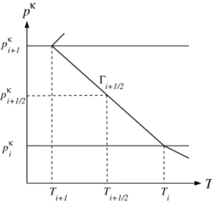
Let us assume that temperature dataT1,T2,. . .Ti,. . .Tnare available at pressure levelsp1,p2,. . .pi,. . .pn(see Figure 1). 1

Now at Geophysical Fluid Dynamics Laboratory/Princeton University, Princeton, New Jersey, USA.

(2)

We then calculatei+1/2at the half levels whose pressure is given by pk_i_þ₁₌₂¼p k iþp k iþ1 2 : ð3Þ

We approximate (2) by finite differences assuming that T

varies linearly withpk, so that the lapse-rate at the half levels is calculated as iþ1=2¼ Tiþ1Ti ð Þ pk iþ1p k i p k i þp k iþ1 TiþTiþ1 ð Þ kg R ð4Þ

[7] Having determined the lapse-rate at all half levels we construct a continuous profile by interpolating linearly withpk. Starting at the lowest level we then search for that half levelpj+1/2wherej+1/2is smaller than the critical lapse-rateTP= 2 K/km for the first time. We then check whether the mean lapse-rate of the 2 km deep layer above the pressure levelpj+1/2remains belowTP. If the second criterion is not fulfilled, we search for the next half level abovepj+1/2where the lapse-rate is again belowTP. If both criteria are met, the exact position of the tropopause is determined by interpolat-inglinearly withpkbetween the half levelsj1/2 andj+ 1/2. The pressure level where the lapse-rate reaches the critical valueTPdenotes the tropopause pressurepTP:

pkTP¼p k j1=2þ pk jþ1=2p k j1=2 jþ1=2j1=2 TPj1=2 ð5Þ [8] In the event that multiple vertical levels meet these criteria, the tropopause is assigned to the lowest position of occurrence. To avoid unrealistically high or low tropopause heights and to increase computational speed, the search range for the algorithm is limited to between 550 hPa and 75 hPa (approx. 5 – 18 km). If the calculated tropopause exceeds one of these limits, the result is rejected and the tropopause is assigned the missing value at this grid point. After the tropopause has been calculated for all horizontal grid points, one can optionally fill in missing values by the mean of their surrounding points. The reader can find a program of the above algorithm at http://www.gfdl.noaa. gov/~tjr/TROPO/tropocode.htm.

3. Evaluation

[9] Using the algorithm described in section 2, we calculated tropopause heights from ECMWF analyses and compared them with heights reported from radiosonde

stations. The goal was to (1) test the algorithm, and (2) to find out whether coarsely resolved analyses are suitable input data.

3.1. Data

[10] The observational data were operationally reported tropopause heights from radiosonde stations. At the station, the tropopause is determined by visual inspection of the highly resolved temperature profile using the WMO crite-rion. The verification was performed using observed daily height data for six individual months: January and July of 1992, 1993 and 1994. To calculate the tropopause, we used daily temperatures of standard analyses from ECMWF in T42 resolution [ECMWF, 1993]. The spectral data were transformed to a grid with a resolution of roughly 2.8 2.8degrees. In the vertical, we used 10 standard isobaric surfaces from 700 – 50 hPa.. It is likely that most or perhaps all of the radiosonde data used for the verification were assimilated in the ECMWF-analyses, so that both calculated and observed tropopause heights were based on similar input data.

[11] As mentioned above, occasionally no tropopause could be determined, either because the WMO criteria were not met, or because the calculated height exceeded the lower or upper limit. However, the failure rate was fairly low: The tropopause height could not be determined in only 0.1% of all cases. The vast majority of these cases occurred over the Antarctic between June and September, with a pronounced maximum in July. At this location and time, the failure rate approached 16%. This was related to extremely cold tropospheric temperatures during Antarctic winter, which produced a relatively isothermal temperature struc-ture in the stratosphere and mid- to upper troposphere [see, e.g., Highwood et al., 2000]. Over the Arctic during northern winter, the calculation of the tropopause also failed at times, but far less frequently than over the Antarctic. The local failure rate was smaller than over Antarctica with local maxima of up to 1.4%.

[12] Figure 2 shows the distribution of the 340 regularly reporting (Ndays 15) stations that were used for the evaluation. The coverage was sparse at high latitudes and the tropics, and rather dense in the extratropics. We performed a simple quality control on the station data to remove obvious errors. For each selected station, up to Figure 1. TemperatureTas a function of pressurep.

Figure 2. Distribution of the 340 regularly reporting (15 reports per month) upper-air stations.

(3)

6 monthly time series (i.e., the three Januarys and three Julys of 1992, 1993 and 1994) were obtained, each of them containing up to 31 daily tropopause values.

[13] For the stations considered here, the monthly time series of tropopause heights contained different numbers of daily reports. Before comparing with analyses, therefore, we required that the number of valid tropopause reports (Ndays) was at least 15 out of a possible 31. This yielded a total of 1511 monthly time series of tropopause height (744 for January, 767 for July) from 340 different stations (314 for January, 294 for July). On average, 26 reports were available for each month. We also performed our compar-ison of calculated and reported tropopause heights with more stringent requirements for the treatment of missing data. We did this by incrementally increasing the minimum number of valid tropopause reports from 15 to 28, and by restricting our attention to results from stations which satisfied these criteria in all 6 months. The results of the evaluation were relatively insensitive to the choice of missing data criteria.

3.2. Results

[14] To eliminate small scale features, means of 2 2 grid-point data of calculated tropopause heights were used for the evaluation. To account for gaps in temporal cover-age, the calculated heights from ECMWF analyses were masked with the temporal coverage at the location of the radiosonde stations.

[15] For an objective comparison it was desirable to combine several reported tropopause heights to the same 5.6 5.6 area averages as the calculated heights. This was only possible over data-rich areas. Here, we examine in detail a region of this type. It is located over Europe and

covers about 500 km 600 km. This region includes 8 regularly reporting stations that are homogeneously dis-tributed. Figure 3 depicts January time series of calculated (top) and measured (middle) area mean tropopause heights, and their differences (bottom).

[16] The agreement between calculated and measured tropopause values is rather good. The strong fluctuations of measured tropopause pressures, which are typical of extratropical synoptic activity, are reproduced well by the calculations. The bottom graphs show that the deviations are, in general, within the spatial standard deviation of measured tropopause pressure. For all 3 January time series combined, the bias in calculated tropopause pressure amounts to 3 hPa with a spatial standard deviation of 11 hPa. In July, when synoptic activity and tropopause variability is smaller, the mean difference amounts to 1 hPa and its spatial standard deviation to 9 hPa (not shown). Further detailed comparisons can be found in Reichler

[1995]. The excellent agreement between calculations and measurements illustrates that our algorithm, which relies on interpolation of lapse-rates, can provide reliable estimates of tropopause height despite the coarse vertical resolution of the input data. An important prerequisite, however, was the high observation density, which ensured that both analyses and observations were reliable and representative.

[17] Figure 4 shows the results of the evaluation from all stations for January and July 1992 – 1994 as a function of station latitude. Depicted are monthly mean differences between station reports and corresponding 22 grid-point means derived from ECMWF-analyses. At many locations, the comparisons involved single station data only, and hence were necessarily noisier than the regional average shown in Figure 3.

Figure 3. Tropopause pressure over central Europe (47– 53N, 07– 12E) during January 1992 – 94 as calculated from analyses (top) and as measured from radiosondes (middle). ‘+’-symbols mark individual grid-point calculations or radiosonde measurements, and the full lines shows area means. The bottom panels show the differences (full line, calculated minus measured), and the spatial standard deviation (dotted line). The monthly spatial standard deviation (s) and the monthly mean (m) are specified in hPa.ndenotes the number of reports.

(4)

[18] The error structure is to first order symmetric about the equator. Based on this structure, we divided the results into 1 tropical (25S – 25N), 2 subtropical (26 – 44) and 2 extratropical zones (45 – 90) and calculated the statistics in each zone (Table 1). In the extratropics, the differences are rather small compared to the mean tropopause pressure of about 250 hPa. In the Northern Hemisphere extratropics, the mean rms-error is 27 hPa in January and 20 hPa in July. The relatively few stations over the southern extratropics yield similar results. During January, the deviations scatter quite evenly around zero, whereas in July there is a tendency towards positive deviations with latitude. Over the tropics, the mean rms-error is 17 hPa in January and 13 hPa in July. Considering the low tropopause pressure in the tropics (100 hPa), the relative error equals to 13 – 17%. The two subtropical zones have rather large deviations with rms-errors between 29 and 54 hPa. This is probably related to a sharp transition zone from the high tropical to the low extratropical tropopause in this latitude band, which cannot be adequately resolved by the analyses. Figures 4 also show that the position of maximum differences shifts by 10to the North from January to July, which is in good agreement with the seasonal shift of the major meridional overturning cells.

4. Summary and Conclusions

[19] We developed and tested an algorithm involving interpolation of lapse-rates to determine the height of the

tropopause from coarsely resolved temperature data. The algorithm uses a thermal definition of the tropopause, and is based on the standard WMO lapse-rate criterion. It can easily be applied to any type of analyses or model output, and it can also directly be implemented into models to study cross tropopause transport. The method was evaluated by comparing the heights calculated from ECMWF-analyses with observed heights at individual stations. In the extra-tropics, the mean rms-error of daily heights was on the order of 30 – 40 hPa. In the tropics, the mean rms-error was about 15 hPa. Deviations of up to 60 hPa were found in the subtropics of both hemispheres. These are most likely associated with strong meridional gradients in tropopause height. Clearly, the accuracy of the method is limited by the resolution of the input data, which is usually too coarse to resolve regional structures and the steep tropopause gra-dients in the tropical-extratropical transition zone. It should also be noted that the differences between observed and calculated heights are not solely attributable to the coarse vertical resolution of the input data. Other factors like differences in temporal and spatial sampling, and changes over time in the analysis model may also be responsible. Overall, these results are encouraging, in particular when considering the coarse vertical resolution of the input data. Improvements can be expected with the use of temperature data with higher vertical resolution in the vicinity of the tropopause.

[20] Acknowledgments. We would like to thank Ben Santer for his comments which greatly helped to improve the original manuscript. We are grateful to the Institut fu¨r Meteorologie, Freie Universita¨t Berlin, for the provision of the radiosonde data. The ECMWF-analyses were used by permission of the Deutscher Wetterdienst, Offenbach. This study was partly supported by the Bundesministerium fu¨r Bildung, Wissenschaft, Forschung und Technologie, Bonn, under grant 01 LO 9215.

References

ECMWF, The description of the ECMWF/WCRP Level III global atmo-spheric data archive, ECMWF, Reading, United Kingdom, 49 pp., ECMWF, Shinfield Park, Reading RG29AK, UK, 1993.

Grewe, V., and M. Dameris, Calculating the global mass exchange between stratosphere and troposphere,Ann. Geophysicae,14, 431 – 442, 1996. Highwood, E. J., B. J. Hoskins, and P. Berrisford, Properties of the Arctic

tropopause,Q. J. R. Meteorol. Soc.,126, 1515 – 1532, 2000.

Hoerling, M. P., T. K. Schaack, and A. J. Lenzen, Global objective tropo-pause analysis,Mon. Wea. Rev.,119, 1816 – 1831, 1991.

Holton, J. R., P. H. Haynes, M. E. McIntyre, A. R. Douglass, R. B. Rood, and L. Pfister, Stratosphere-troposphere exchange,Rev. Geophys.,33, 403 – 439, 1995.

Reichler, T., Eine globale Klimatologie der Tropopausenho¨he auf der Basis von ECMWF-Analysen, Diploma thesis at the University of Augsburg, Germany, 145 pp., 1995.

Reiter, E. R., Stratospheric-tropospheric exchange processes,Rev. Geophys. Space Phys.,13, 459 – 474, 1975.

Santer, B. D., R. Sausen, T. M. L. Wigley, J. S. Boyle, K. AchutaRao, C. Doutriaux, J. E. Hansen, G. A. Meehl, E. Roeckner, R. Ruedy, G. Schmidt, and K. E. Taylor, Behavior of tropopause height and atmo-spheric temperature in models, reanalyses, and observations: Decadal changes,J. Geophys. Res.,108(D1), 4002, doi:10.1029/2002JD002258, 2003a.

Figure 4. Monthly mean differences between calculated and measured tropopause pressures. Thin vertical lines denote temporal standard deviation of daily differences (±s), derived from all available time series of a specific station. The x-axis denotes latitudinal position of the stations.

Table 1. Mean bias (m) and rms-error in hPa of model derived tropopause pressure, averaged over the 5 latitudinal zones January 90 – 45S 44 – 26S 25S – 25N 26 – 44N 45 – 90N m 11 3 9 7 3 rms 26 32 17 42 27 July 90S – 45S 44S – 26S 25S – 25N 26 – 44N 45 – 90N m 6 12 4 2 3 rms 31 54 13 29 20

(5)

Santer, B. D., M. F. Wehner, T. M. L. Wigley, R. Sausen, G. A. Meehl, K. E. Taylor, C. Ammann, J. Arblaster, W. M. Washington, J. S. Boyle, and W. Bru¨ggemann, Contributions of anthropogenic and natural for-cing to recent tropopause height changes, Science, 301, 479 – 483, 2003b.

Sausen, R., and B. D. Santer, Use of changes in tropopause height to detect human influences on climate,Meteorol. Z.,12, 131 – 136, 2003. Shepherd, T. G., Issues of stratosphere-troposphere coupling,J. Met. Soc.

Japan,80(4B), 769 – 792, 2002.

Stuber, N., R. Sausen, and M. Ponater, Stratosphere adjusted radiative forcing calculations in a comprehensive climate model,Theor. Appl. Climato,68, 125 – 135, 2001.

Thuburn, J., and G. Craig, GCM tests of theories for the height of the tropopause,J. Atmos. Sci.,54, 869 – 882, 1997.

World Meteorological Organization (WMO), Meteorology A Three-Dimen-sional Science: Second Session of the Commission for Aerology,WMO Bulletin IV(4), WMO, Geneva, 134 – 138, 1957.

T. Reichler, Geophysical Fluid Dynamics Laboratory, Princeton Uni-versity, Princeton, NJ, USA. ([email protected])

M. Dameris and R. Sausen, Institut fu¨r Physik der Atmospha¨re, Deutsches Zentrum fu¨r Luft- und Raumfahrt, Oberpfaffenhofen, Germany.