10 GEOMETRIC DISTRIBUTION EXAMPLES:

(1)

1. Terminals on an on-line computer system are at-tached to a communication line to the central com-puter system. The probability that any terminal is ready to transmit is 0.95.

Let X = number of terminals polled until the first ready terminal is located.

2. Toss a coin repeatedly.

Let X = number of tosses to first head

3. It is known that 20% of products on a production line are defective. Products are inspected until first defective is encountered.

Let X = number of inspections to obtain first defec-tive

4. One percent of bits transmitted through a digital transmission are received in error. Bits are trans-mitted until the first error.

Let X denote the number of bits transmitted until the first error.

(2)

GEOMETRIC DISTRIBUTION Conditions:

1. An experiment consists of repeating trials until first success.

2. Each trial has two possible outcomes; (a) A success with probability p

(b) A failure with probability q = 1−p. 3. Repeated trials are independent.

X = number of trials to first success

X is a GEOMETRIC RANDOM VARIABLE.

PDF: P(X = x) =qx−1 p; x = 1,2,3,· · · CDF: P(X ≤x) = P(X = 1) + P(X = 2)· · ·P(X = x) = p+qp+q2p· · ·+qx−1 p = p[1−qx ]/(1−q) = 1−qx

(3)

Example:

Products produced by a machine has a 3% defective rate.

• What is the probability that the first defective oc-curs in the fifth item inspected?

P(X = 5) = P(1st 4 non-defective )P( 5th defective) = 0.974 (0.03) In R >dgeom (x= 4, prob = .03) [1] 0.02655878

The convention in R _{is to record} _X _{as the number} of failures that occur before the first success.

• What is the probability that the first defective oc-curs in the first five inspections?

P(X ≤ 5) = 1−P(First 5 non-defective) = 1−0.975

> pgeom(4, .03) [1] 0.1412660

(4)

Geometric pdf s

1 2 3 4 5

0.0

0.4

0.8

First Ready Terminal, p = .95

X = Number of Trials P(X=x) 2 4 6 8 10 0.0 0.2 0.4 First Head, p = .5 X = Number of Trials P(X=x) 5 10 15 20 0.00 0.10 0.20 First Defective, p = .2 X = Number of Trials P(X=x) 0 100 200 300 400 0.000 0.004 0.008

First Bit in Error, p = .01

X = Number of Trials

(5)

Calculating pdfs in R

par (mfrow = c(2,2)) x<-0:4

plot(x+1, dgeom(x, prob = .95),

xlab = "X = Number of Trials", ylab = "P(X=x)", type = "h", main = "First Ready Terminal, p = .95") x<-0:9

xlab = "X = Number of Trials", ylab = "P(X=x)", type = "h", main = "First Head, p = .5")

x<- 0:19

xlab = "X = Number of Trials", ylab = "P(X=x)", type = "h", main = "First Defective, p = .2")

x<- seq(0, 400, 50)

xlab = "X = Number of Trials", ylab = "P(X=x)", type = "h", main = "First Bit in Error, p = .01")

(6)

1 2 3 4 5

0.95

0.98

First Ready Terminal, p = .95

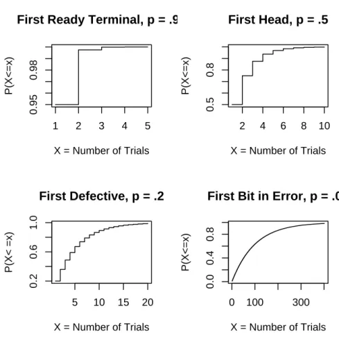
X = Number of Trials P(X<=x) 2 4 6 8 10 0.5 0.8 First Head, p = .5 X = Number of Trials P(X<=x) 5 10 15 20 0.2 0.6 1.0 First Defective, p = .2 X = Number of Trials P(X< =x) 0 100 300 0.0 0.4 0.8

First Bit in Error, p = .01

X = Number of Trials

P(X<=x)

(7)

par (mfrow = c(2,2)) x<-0:4

plot(x+1, pgeom(x, prob = .95),

xlab = "X = Number of Trials", ylab = "P(X<=x)", type = "s", main = "First Ready Terminal, p = .95") x<-0:9

xlab = "X = Number of Trials", ylab = "P(X<=x)", type = "s", main = "First Head, p = .5")

x<-0:19

xlab = "X = Number of Trials", ylab = "P(X< =x)", type = "s", main = "First Defective, p = .2") x<- seq(0, 399)

xlab = "X = Number of Trials", ylab = "P(X<=x)", type = "s", main = "First Bit in Error, p = .01")

(8)

The Quantile Function

In Example 3, a production line which has a 20% defec-tive rate, what is the minimum number of inspections, that would be necessary so that the probability of ob-serving a defective is more that 75%?

Choose k so that

P(X ≤ k) ≥ .75. In R

qgeom(.75, .2) [1] 6

i.e. 6 failures before first success.

or with 7 inspections, there is at least a 75% chance of obtaining the first defective.

(9)

Mean of geometric distribution: Example:

If a production line has a 20% defective rate. What is the average number of inspections to obtain the first defective? E(X) = X∞ x=1 xqx−1 p = p X∞ x=1 xqx−1 = p ∞ X x=1 dqx dq = pd P∞ x=1q x dq = pd(q/(1−q) dq = p[(1−q) +q] (1−q)2 = p p2 = 1 p

Average number of inspections to obtain the first defec-tive:

E(X) = 1 .2 = 5

(10)

The Markov Property:

If the probability of events happening in the future is independent of what went before, then the random vari-able is said to have the Markov property.

MARKOV PROPERTY =⇒ MEMORYLESS PROPERTY Example:

Products are inspected until first defective is found. X is a geometric random variable with parameter p. The first 10 trials have been found to be free of defectives. What is the probability that the first defective will occur in the 15th trial?

Let E1 be the event that first ten trials are free of

defec-tives.

Let E2 be the event that that first defective will occur

on the 15th trial. P(X = 15|X > 10) = P(E2|E1) = P(E1 ∩E2) P(E1) = P(X = 15∩X > 10) P(X > 10) = P(X = 15) P(X >10) = q 14_p q10 = q 4_p₌ _P_(X _{= 5)}

(11)

MARKOV PROPERTY

Generally, the Markov property states:

P(X = x+n|X > n) = P(X = x) Proof:

Let

E1 = {X > n}

E2 = {X = x+n}

Then we may write

(12)

R _{Functions for the Geometric Distribution}

• dgeom

dgeom (x= 4, prob = .03)

the probability of

exactly 4 trials before first defective or exactly 5 trials to first defective

• pgeom

pgeom (x= 4, prob = .03)

the probability of

up to 4 trials before first defective or up to 5 trials to first defective

• qgeom

qgeom(.75, .2)

returns the number of trials before first defective that has a probabilty of .75.