OPTIMAL WEIGHTING FACTOR FOR SINGLE-STEP TRAPEZOIDAL METHOD

OPTIMAL WEIGHTING FACTOR FOR SINGLE-STEP TRAPEZOIDAL METHOD

Fuzhang Zhao

Department of Mechanical Engineering, Temple University 1947 N. 12th Street, Philadelphia, Pennsylvania 19122, USA

Phone: (215) 204-7805, Fax: (215) 204-4956, and e-mail: [email protected] ABSTRACT

A new optimal weighting factor for a single-step trapezoidal method, θ = 0.618, has been developed to solve transient linear and nonlinear heat conduction problems. The numerical results based on the optimal weighting factor developed, through both linear and nonlinear benchmark tests, are compared with other commonly used single-step trapezoidal methods with emphasis on the combination of both accuracy and efficiency in the solution. The optimal weighting factor of single-step method has been proved to be very accurate, stable, and efficient. The relevant features for the single-step trapezoidal methods are also addressed.

INTRODUCTION

A first-order parabolic system governs many engineering problems. A typical example is the transient heat conduction problems. In solving such a system, there are two families of algorithms: trapezoidal and exponential. The single-step trapezoidal methods are more widely used when dealing with the time dimension in finite element method. The most commonly used single-step trapezoidal methods include the Euler forward and backward methods [1], the Crank-Nicolson method [2], the Liniger method [3], and the Galerkin method [4]. The generalized trapezoidal family of algorithms along with the two-step methods and three-step methods has been summarized in reference [5]. For the exponential family of algorithms, an exponential scheme was developed by Patankar and Baliga [6], a finite-analytic method also using exponential analytic function was developed by Chen and Li [7], and a further exponential family of algorithm was generalized by Mercer [8]. The early work was focused on the accuracy of the calculations. As the problems become more and more time consuming, it becomes clear that the efficiency of the solution is just as important as its accuracy. In order to use a relatively large time step without losing solution accuracy, an optimal single-step exponential scheme was developed by Li [9]. A good review of exponential schemes can be found in reference [9]. The single-step exponential methods are mainly used in finite difference method.

In numerical simulations of transient heat conduction problems using finite element methods, the single-step trapezoidal families of algorithms are usually adopted. To increase the solution efficiency for time-dependent problems, a larger time step with a simple formulation is preferred. If the time step used is too large, however, accuracy may be sacrificed. Therefore, in order to have balanced accuracy and efficiency, the weighting factor needs to be optimized for the single-step trapezoidal method. An optimal weighting factor for single-step algorithms has been developed. To demonstrate the validity of the optimal weighting factor, two-benchmark problems having analytical solutions are selected and studied. Those problems have also been solved numerically using single-step trapezoidal methods. Results based on the Euler forward and backward methods, the Crank-Nicolson method, the Galerkin method, and the optimal weighting factor of single-step method are compared and discussed with an emphasis on the combination of both solution accuracy and solution efficiency.

FORMULATIONS

In finite element formulation, the discretization of space and time can be conducted separately. A general finite element governing equation for transient heat conduction problems after discretization on space reads [10]:

[ ]

C

{ }

T& +

[ ]

K

{ } { }

T = Q

( )

1 where [C] is the capacity matrix, [K] is the conductivity matrix, {Q} is the thermal load vector, {T} is temperature vector, and {T&} is the vector of the derivative of temperature with respect to time.

With time discretization using the single-step trapezoidal method, Eq. (1) takes the following form [11]:

[ ] [ ]

{ }

[ ]

(

)

[ ]

{ } {

}

(

1

){ } ( )

2 1 t t t t t t Q Q T K t C T K t C θ θ θ θ − + +       _{− −} ∆ =       ₊ ∆ +∆ +∆ Proceedings of IMECE’03 2003 ASME International Mechanical Engineering Congress Washington, D.C., November 15–21, 2003

where {Qt} and {Qt+∆t} denote the thermal load vectors at times t and t + ∆t, respectively, and θ is a weighting factor bounded

within the interval [0, 1]. In the Euler forward and backward methods, θ is 0 and 1, respectively. The Crank-Nicolson method uses θ = 0.5 and the Galerkin method uses θ = 2/3 [10]. When the Galerkin method, for example, is used in transient heat conduction problems, it means that within any single time step, the weight for temperature/thermal load at future time, t + ∆t, is 1/3 and the weight for temperature/thermal load at current time, t, is 2/3.

The Golden Section is found to be useful for optimization [12]. The optimal weighting factor of single-step trapezoidal method can be obtained by the application of Golden Section. It requires that the weight for temperature/thermal load at future time, t + ∆t, over the weight for temperature/thermal load at current time, t, be balanced with the weight for temperature/thermal load at current time over the weight for temperature/thermal load within the whole single time step:

( )

3 1 1 θ θ θ = − Rearranging Eq. (3) yields

( )

4 0

1

2_{+θ− =}

θ

Solving Eq. (4) gives the positive root:

( )

5 618 . 0 2 1 5− _≈ = θ

When Eq. (5) is used in Eq. (2), the optimal weighting factor of single-step trapezoidal method is established for finite element analysis.

It is interesting to find that all the most commonly used weighting factors in the single-step trapezoidal method can be defined by the ratio of Fibonacci sequence (0, 1, 1, 2, 3, 5, 8, 13, 21, 34, 55, 89, 144, 233, 377, 610, 987…). The Euler forward method has the weighting factor of θ = 0 = F0/F1. The

Euler backward method has the weighting factor of θ = 1 =

F1/F2. The Crank-Nicolson method uses the weighting factor of

θ = 0.5 = F2/F3. The Galerkin method uses the weighting factor

of θ = 2/3 = F3/F4. The optimal weighting factor can also be

obtained by the ratio of Fibonacci sequence Fn. As the term

index n further increases, the weighting factor approaches to θ

= Fn-1/Fn=0.618.

EVALUATION OF ACCURACY AND EFFICIENCY

In order to demonstrate the validity of the optimal weighting factor of single-step method, two benchmark examples with exact solutions are selected for comparison. One example is a linear problem and the other is a nonlinear problem. In both cases, the analytical solution of the temperature profile is developed first. Then the same problem is solved by all the single-step methods including the optimal weighting factor of single-step method. Finally, the numerical results are compared with the analytical results with emphasis on both the solution accuracy and efficiency.

Only a finite number of elements can be discretized in finite element analysis. Using a finite number of elements to model a continuum medium will create errors. In order to eliminate the error due to the discretization of space, the benchmark problems were selected without the influence of space dimensions. In this way, the governing equation, Eq. (1), becomes a one degree equation:

( )

6

Q KT T C&+ =

The first example involves an adiabatic system with initial temperature of one. As time elapses, the temperature variations fade away and eventually the temperature reaches the steady-state temperature, i.e., zero. Setting C = K = 1, Q = 0, initial condition of T(0) = 1 and solving yields the most commonly used linear benchmark problem with the following analytical solution [10]:

( )

7 )

(_{t e} t

T ₌ −

With Eq. (2), the recurrence relationship for the numerical solution of Example 1 can be readily obtained:

(

)

( )

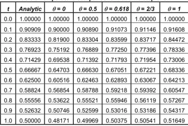
8 1 1 1 t t t T t t T ∆ + ∆ − − = ∆ + _θ θ

The results calculated from Eq. (8) with different time steps, ∆t, using the Euler forward method (θ = 0), the Crank-Nicolson method (θ = 0.5), the optimal weighting factor of single-step method (θ = 0.618), the Galerkin method (θ =2/3), and the Euler backward method (θ =1) are compared with the analytical solution given in Eq. (7). For the time step chosen as small as 0.1, the results are listed in Table 1. The results in Table 1 show that when the small time step of 0.1 is used, all single-step methods give acceptable results and the Crank-Nicolson method is the most accurate. As the time step increases to 1.5, the optimal method has the best accuracy shown in Figure 1. If the time step is further increased to 2.5, all single-step methods have a poor accuracy shown in Figure 2 but the Galerkin method is the closest. The results with time step of 2.5 based on the Euler forward method are out of the window of Figure 2, therefore they are not shown.

Table 1 Temperature comparisons with time step of 0.1

t Analytic θ = 0 θ = 0.5 θ = 0.618 θ = 2/3 θ = 1 0.0 1.00000 1.00000 1.00000 1.00000 1.00000 1.00000 0.1 0.90484 0.90000 0.90476 0.90582 0.90625 0.90909 0.2 0.81873 0.81000 0.81859 0.82051 0.82129 0.82645 0.3 0.74082 0.72900 0.74063 0.74324 0.74429 0.75131 0.4 0.67032 0.65610 0.67010 0.67324 0.67452 0.68301 0.5 0.60653 0.59049 0.60628 0.60983 0.61128 0.62092 0.6 0.54881 0.53144 0.54854 0.55240 0.55397 0.56447 0.7 0.49659 0.47830 0.49630 0.50037 0.50204 0.51316 0.8 0.44933 0.43047 0.44903 0.45325 0.45497 0.46651 0.9 0.40657 0.38742 0.40626 0.41056 0.41232 0.42410 1.0 0.36788 0.34868 0.36757 0.37190 0.37366 0.38554

Figure 1 Temperature comparisons with time step of 1.5.

Figure 2 Temperature comparisons with time step of 2.5.

Figure 3 Performance of different algorithms for Example 1.

The absolute error e1 between numerical and analytical

solutions for the first time step for Example 1 can be calculated as a function of time step ∆t with different weights θ:

(

)

_{( )}

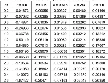
₉ 1 1 1 1 t e t t e ₋ −∆ ∆ + ∆ − − = θ θ

Table 2 Absolute error e1 as a function of θ and ∆t.

∆t θ = 0.0 θ = 0.5 θ = 0.618 θ = 2/3 θ = 1.0 0.2 -0.01873 -0.00055 0.00327 0.00480 0.01460 0.4 -0.07032 -0.00365 0.00897 0.01389 0.04397 0.6 -0.14881 -0.01035 0.01349 0.02262 0.07619 0.8 -0.24933 -0.02076 0.01535 0.02893 0.10623 1.0 -0.36788 -0.03455 0.01409 0.03212 0.13212 1.2 -0.50119 -0.05119 0.00980 0.03214 0.15335 1.4 -0.64660 -0.07013 0.00283 0.02927 0.17007 1.6 -0.80190 -0.09079 -0.00638 0.02391 0.18272 1.8 -0.96530 -0.11267 -0.01739 0.01652 0.19184 2.0 -1.13534 -0.13534 -0.02976 0.00752 0.19800 2.2 -1.31080 -0.15842 -0.04314 -0.00270 0.20170 2.4 -1.49072 -0.18163 -0.05718 -0.01379 0.20340 2.6 -1.67427 -0.20471 -0.07163 -0.02549 0.20350 The calculated absolute error e1 as a function of both the

weight θ and time step ∆t is listed in Table 2. For the cases of θ = 0, 0.5, and 1, the error increases monotonically with time-step. For the cases of θ = 0.618 and 2/3, the zero-errors can be located at the time steps of 1.46640935 and 2.14912570, respectively.

To demonstrate the variation trends of e1 as a function of

both the weight θ and time step ∆t, the results based on Eq. (9) have also been plotted in Figure 3.

In order to demonstrate the solution accuracy and efficiency of the proposed optimal weighting factor for nonlinear problems, a transient heat conduction problem with thermal conductivity as a function of temperature, which makes the problem nonlinear, is considered in the second benchmark example problem. The second example problem is similar to the first one physically. The thermal conductivity is selected to be T. Setting C = 1, Q = 0, and K = T, substituting them into Eq. (6), applying initial condition of T(0) = 1 and solving yield the nonlinear benchmark problem with the following analytical solution:

( )

10 1 1 ) ( + = t t T

With Eq. (2), the recurrence relationship for Example 2 can be obtained:

(

)

(

1

)

(

1

)

( )

11 1 1 1 2 2 t t t t t t t t t T T T t T T T t       _{− − − −} ∆ =       _{+ − +} ∆ ∆ + ∆ + ∆ + θ θ θ θ θ θ

With the derivative of Eq. (11) with respect to Tt+∆t and

expansion of linear Taylor series, the equation for Example 2 using Newton-Raphson iteration method turns out to be [10]:

(

)

(

1

)

(

1

)

( )

12 2 2 1 2 1 2 2 2 2 2       _{− − − − −} ∆ − = ∆       _{+ − +} ∆ ∆ + ∆ + ∆ + ∆ + t t t t t t t t t t t t T T T T t T T T T T t θ θ θ θ θ θ θ

The convergence of the solution during the iteration process is measured by the temperature difference for Example 2. The iteration stops when the absolute value of temperature difference at the current iteration is smaller than a designated small positive number – convergent limit:

( )

13 ε

< ∆_Ti

where i denotes the iteration number. In the present example, 5 iterations are required under the convergent condition of ε = 10–8_{. The initial guess of temperature T}

t+∆t is set to zero at all

different times.

Similar to the linear case, the temperature results calculated from Eq. (12) with different time steps, ∆t, using all the mentioned single-step methods are compared with the analytical solution Eq. (10). For the time step chosen as small as 0.1, the results are listed in Table 3. It shows that when the small time step of 0.1 is used, all single-step methods give acceptable results and the Crank-Nicolson method has the best accuracy. As the time step used increases to 1.5, the optimal weighting factor of single-step method has the best accuracy shown in Figure 4. If the time step is further increased to 2.5, all single-step methods have a poor accuracy shown in Figure 5, but the Galerkin method is the closest again. Since the results with a time step of 2.5 based on the Euler forward method are out of the window of Figure 5, no data are shown.

Table 3 Temperature comparisons with time step of 0.1

t Analytic θ = 0 θ = 0.5 θ = 0.618 θ = 2/3 θ = 1 0.0 1.00000 1.00000 1.00000 1.00000 1.00000 1.00000 0.1 0.90909 0.90000 0.90890 0.91073 0.91146 0.91608 0.2 0.83333 0.81900 0.83304 0.83599 0.83717 0.84472 0.3 0.76923 0.75192 0.76889 0.77250 0.77396 0.78336 0.4 0.71429 0.69538 0.71392 0.71793 0.71954 0.73006 0.5 0.66667 0.64703 0.66630 0.67051 0.67221 0.68336 0.6 0.62500 0.60516 0.62463 0.62893 0.63067 0.64213 0.7 0.58824 0.56854 0.58788 0.59218 0.59392 0.60547 0.8 0.55556 0.53622 0.55521 0.55946 0.56119 0.57267 0.9 0.52632 0.50746 0.52599 0.53016 0.53186 0.54317 1.0 0.50000 0.48171 0.49969 0.50375 0.50541 0.51649 The temperature after the first time step can also be formulated by solving Eq. (11) analytically. The absolute error between analytical and numerical solutions for the first time step for Example 2, then, can be estimated as a function of both time step ∆t and weighting factors θ:

(

)

(

)

(

(

)

)

(

(

)

)

( )

14 1 1 2 1 2 1 1 1 4 1 2 1 2 2 2 2 2 + ∆ − ∆ ∆ − + − ∆ − − ∆ + ∆ − + = t t t t t t e θ θ θ θ θ θ θ

Figure 4 Temperature comparisons with time step of 1.5.

Figure 5 Temperature comparisons with time step of 2.5.

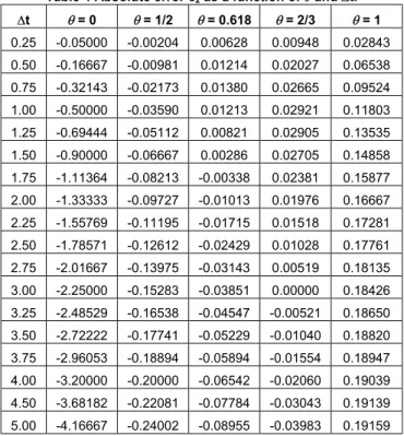
The calculated absolute error e2 as a function of both the

weight θ and time step ∆t is listed in Table 4. For the cases of θ = 0, 0.5, and 1, the error increases monotonically with time-step. For the cases of θ = 0.618 and 2/3, the zero-errors can be located at time steps of 1.61803399 and 3.00000000, respectively. To demonstrate the variation trends of e2 as a

function of both the weight θ and time step ∆t, the results based on Eq. (14) have also been depicted in Figure 6.

Table 4 Absolute error e2 as a function of θ and ∆t.

∆t θ = 0 θ = 1/2 θ = 0.618 θ = 2/3 θ = 1 0.25 -0.05000 -0.00204 0.00628 0.00948 0.02843 0.50 -0.16667 -0.00981 0.01214 0.02027 0.06538 0.75 -0.32143 -0.02173 0.01380 0.02665 0.09524 1.00 -0.50000 -0.03590 0.01213 0.02921 0.11803 1.25 -0.69444 -0.05112 0.00821 0.02905 0.13535 1.50 -0.90000 -0.06667 0.00286 0.02705 0.14858 1.75 -1.11364 -0.08213 -0.00338 0.02381 0.15877 2.00 -1.33333 -0.09727 -0.01013 0.01976 0.16667 2.25 -1.55769 -0.11195 -0.01715 0.01518 0.17281 2.50 -1.78571 -0.12612 -0.02429 0.01028 0.17761 2.75 -2.01667 -0.13975 -0.03143 0.00519 0.18135 3.00 -2.25000 -0.15283 -0.03851 0.00000 0.18426 3.25 -2.48529 -0.16538 -0.04547 -0.00521 0.18650 3.50 -2.72222 -0.17741 -0.05229 -0.01040 0.18820 3.75 -2.96053 -0.18894 -0.05894 -0.01554 0.18947 4.00 -3.20000 -0.20000 -0.06542 -0.02060 0.19039 4.50 -3.68182 -0.22081 -0.07784 -0.03043 0.19139 5.00 -4.16667 -0.24002 -0.08955 -0.03983 0.19159 The results based on both the linear case Eq. (9) and the nonlinear case Eq. (14) show that all single-step methods have very good accuracy at small time steps. As the time step increases from small to relatively large, the optimal weighting factor of single-step method has the best accuracy among all the different weighting factors used. Although the Galerkin method can be used with a larger time step than the optimal method, the overall accuracy of Galerkin method is poorer than the optimal method. As time step further increases all methods perform poorly in accuracy although the solution efficiency is better. Both the optimal and Galerkin methods have zero-error points. This means that both methods could have the accuracy of an exact solution if an appropriate time step can be predicted. If the optimal weighting factor is used for both linear and nonlinear benchmark tests, zero error can be achieved at time steps of 1.46640935 and 1.61803399, respectively. If the Galerkin weighting factor is used, zero error can be achieved when the time steps are, respectively, 2.14912570 and 3.00000000. When the optimal weighting factor is used for both linear and nonlinear cases, the time step is nearly equal and equal to the golden ratio of ϕ = 1.61803399, respectively. This result can be extended to the more general case. When the optimal weighting factor is used, the time step can be chosen based on the following equation:

( )

15 2 L k c t=ϕ ρ ∆

where ρ is a density, c is a specific heat, k is a thermal conductivity and L is a characteristic length. The value of L2 _is

one for both the linear and nonlinear benchmark cases.

CONCLUDING REMARKS

The optimal weighting factor for single-step trapezoidal method, θ = 0.618, has been developed to solve transient linear and nonlinear heat conduction problems. The optimal weighting factor of single-step method, through both linear and nonlinear benchmark tests, has been proved to be very accurate, stable, and efficient over a wide range of time steps. When small time step is used the Crank-Nicolson method, θ = 0.5, has the best accuracy for the two benchmark cases but the solution efficiency is low. When the Galerkin method, θ = 2/3, is adopted, the solution efficiency can be improved but the accuracy is decreased.

The Galerkin method can produce the accuracy of the exact solution if the specific time step for a certain problem can be predicted although the prediction for a general problem is difficult. When optimal weighting factor (1/ϕ) is used, however, the near zero or zero error can be achieved with time step equal to the golden ratio (ϕ) for both linear and nonlinear benchmark tests. For general isotropic materials, the time step can be chosen based on Eq. (15).

It is interesting to find that all of the most commonly used weighting factors in single-step trapezoidal methods can be defined by the ratio of the Fibonacci sequence. The optimal weighting factor can also be obtained by the ratio of Fibonacci sequence and as the term index increases, the ratio approaches to the optimal weighting factor.

The optimal weighting factor of single-step trapezoidal method should be readily implemented in the existing commercial packages that use single-step trapezoidal methods since the mathematical framework is the same and the only difference is on the use of weight θ.

ACKNOWLEDGMENTS

The author gratefully acknowledges the support of Temple University. The author came up the concept of the optimal weighting factor for single-step trapezoidal method during his teaching of Finite Element Analysis for graduate students. Thanks are also due to Dr. Richard Cohen, Dr. Jim Chen and Dr. Keya Sadeghipour of Temple University for their encouragement and valuable suggestions.

REFERENCES

[1] Euler, L., 1913, “De Integratione Aequationum Differentialium per Appriximationem,” Opera Omnia, Vol. 11, p. 424.

[2] Crank, J., and Nicolson, P., 1947, “A Practical Method for the Numerical Evaluation of Solutions of Partial Differential Equations of the Heat Conduction Type,” Proc. Cambridge Phil. Soc., Vol. 43, pp. 50-67.

[3] Liniger, W., 1968, “Optimization of a Numerical Integration Method for Stiff System of Ordinary Differential Equations,” IBM Res. Rep. RC2198.

[4] Zlamal, M., 1977, “Finite Element Methods in Heat Conduction Problems,” Academic Press, New York. [5] Tamma, K.K., Zhou, X., and Kanapady, R., 2002, “The

Time Dimension and A Unified Mathematical Framework for First-Order Parabolic Systems,” Numerical Heat Transfer, Part B, Vol. 41, pp. 239-262.

[6] Patankar, S.V., and Baliga, B.R., 1978, “A New Finite– Difference Scheme for Parabolic Differential Equations,” Numerical Heat Transfer, Vol. 1, pp. 27-37.

[7] Chen, C.J., and Li, P., 1979, “Finite Differential Method in Heat Conduction – Application of Analytical Solution Technique,” ASME Paper No. 79-WA/T-50, ASME Winter Annual Meeting, New York.

[8] Mercer, A.M., 1982, “Some New Finite-Difference Scheme for Parabolic Differential Equations,” Numerical Heat Transfer, Vol. 5, pp. 199-210.

[9] Li, S., 1988, “Optimal Exponential Difference Scheme for Solving Parabolic Partial Differential Equations,” Numerical Heat Transfer, Vol. 14, pp. 357-371.

[10] Zienkiewicz, O.C., and Taylor, R.L., 2000, “The Finite Element Method,” 5th ed., Vol. 1, Butterworth-Heinemann, Boston.

[11] Tseng, A.A., and Zhao, F.Z., 1996, “Multidimensional Inverse Transient Heat Conduction Problems by Direct Sensitivity Coefficient Method Using a Finite-Element Scheme,” Numerical Heat Transfer, Part B, Vol. 29, pp. 365-380.

[12] Vadja, S., 1989, “Fibonacci and Lucas Numbers, and the Golden Section: Theory and Applications,” Ellis Horwood, Chichester.