Deep Learning frameworks for Image Quality Assessment

(1)

Deep Learning Frameworks for Image Quality

Assessment

Aparna R

A Thesis Submitted to

Indian Institute of Technology Hyderabad In Partial Fulfillment of the Requirements for

The Degree of Master of Technology

Department of Electrical Engineering

(2)

(3)

(4)

Acknowledgements

I would like to thank my guide Dr. Sumohana Channappayya for his valuable guidance, support, motivation and his patience. I would also like to thank my labmates especially M. Naga Sailaja, S Rajesh, Balasubramanyam Appina, Dendi Sathya Veera Reddy, Kancharla Parimala, Nagabhushan Eswara and Muhammed Shabeer for their worthy suggestions and moral support.

(5)

Dedication

(6)

Abstract

Technology is advancing by the arrival of deep learning and it finds huge application in image processing also. In this thesis work, I implemented image quality assessment techniques using deep learning. Here I proposed two full reference image quality assessment algorithms and two no reference image quality algorithms. Among the two algorithms on each method, one is a supervised methd and the other is in an unsupervised method.

The first proposed method is full reference image quality assessment using autoencoder. Existing literature shows that statistical features of pristine images are affected in presence of the distortion. To learn distortion discriminating features an autoencoder is trained using a large number of pristine images. The autoencoder is shown to learn a good lower dimensional representation of the input. It is shown that encoded distance features have good distortion discrimination properties. The proposed algorithm delivers competitive performance over standard databases.

The second method which I have proposed is a full reference and no reference image quality assessment using deep convolutional neural networks. A network is trained in a supervised manner with subjective scores as targets. The algorithm is shown to perform efficiently for the distortions that are learned while training the model.

The last proposed method is a classification based no reference image quality assessment. Dis-tortion level in an image may vary from one region to another region. We may not be able to view distortion in some part but it may be present in other parts. A classification model is proposed to tell whether a given input patch is of low quality or high quality. It is shown that the aggregate of the patch quality scores has a high correlation with the subjective scores.

(7)

List of Figures

2.1 Basic structure of Neural network and 3D representation of the Convolutional network 4

2.2 Basic structure of Autoencoder . . . 5

2.3 2 class classification problem using SVM . . . 6

2.5 Denoised image from MNIST database . . . 8

4.1 Input image and decoded Image . . . 14

4.2 Scatter plot showing the relation between subjective scores and absolute error between encoded features of the pristine and distorted image. . . 17

4.3 Scatter plot showing the relation between subjective scores and the absolute error between the decoded features of the pristine and distorted image . . . 19

5.1 Block diagram of the FRIQA algorithm . . . 22

5.2 Block diagram of NRIQA algorithm . . . 23

(10)

Chapter 1

Introduction

Image processing is a rapidly evolving field with immense significance in science and engineering. We are living in a digital world where we can find technologies everywhere. Every day we will across different images of different varieties. We have a large number of devices to capture those images. We can get images of sufficient quality even by using the portable mobile phones. But in many of the cases, we will not get the expected quality of images. This is because of many reasons. Since quality is an important criterion for images, image quality assessment becomes a useful research area. Though this thesis I tried exploring some areas of image quality assessment using deep learning.

1.1

Image Quality Assessment

Image quality is a characteristic of an image that measures the perceived image degradation (typi-cally, compared to an ideal or perfect image). Quality assessment can be categorized as subjective quality assessment and objective quality assessment. In subjective quality assessment a number of human subjects are instructed to give the quality of a given image in a defined scales. An algo-rithm is able to predict the subjective quality of a given image is termed to be an objective quality assessment. While performing subjective quality assessment we should consider a number of users, because opinions will vary among subjects. It also going to depend on the lighting conditions, the experience of the subject in quality assessment, distance from the image and so on.

The mean of the opinions are considered as the quality score since opinions vary among subjects. Performing subjective evaluation for all the images practically seems to be quite cumbersome and also expensive. This is the reason for objective quality assessment methods to have become popular.

Image quality assessment techniques are broadly classified into three categories as follows 1. Full reference image quality assessment(FR IQA)

2. Reduced reference image quality assessment(RR IQA) 3. No reference image quality assessment(NR IQA)

1.1.1

Full reference image quality assessment(FRIQA)

In FRIQA both distorted image and the reference image are available for the determination of the quality.

1.1.2

Reduced reference image quality assessment(RRIQA)

In RRIQA we don’t have complete access to the pristine image but rather have certain characteristics of the reference image available which will help in predicting image quality.

(11)

1.1.3

No reference image quality assessment(NRIQA)

In NRIQA or blind quality assessment, we do not have access to the pristine image or its character-istics. NRIQA has a lot of practical applications.

1.2

Deep learning

Deep Learning is a machine learning technique that learns features directly from the data. The data can be image, text,speech or audio. Most deep learning methods used neural network architecture. Hence deep models refer to a deep neural network. The term ’deep’ in deep neural networks refers to the number of hidden layers present in the neural network. One popular neural network model is a convolutional neural network(CNN). Convolutional neural networks are best suited for image data. Basically, we can classify learning techniques into two categories.

1. Supervised learning. 2. Unsupervised learning

1.2.1

Supervised learning

If we are training a specific machine learning task for every input with corresponding target values or labels then it is called supervised learning. Supervised learning methods will try to learn the relation between te input and its target label. Supervised learning can be of regression or classification. If the target represents continuous values, then it is a regression problem. If the target is represented with finite number of classes, then it is a classification problem.

1.2.2

Unsupervised learning

If we are training a specific machine learning task with only input data then it is unsupervised problem. Unsupervised learning methods try to learn the structure of the data or the relationship among the data points. Clustering is one of the unsupervised methods which tries to divide the data into different clusters. So for a new test data, it will match to the appropriate cluster.

(12)

Chapter 2

Background Theory

2.1

Convolutional Neural Network(CNN)

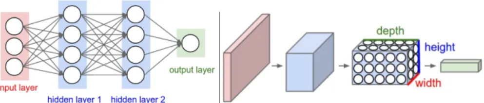
Neural network is one of the machine learning method which is inspired from the human brain. The basic units in a neural network are neurons. There are forward feed neural networks which allow the signal to pass from input to output in a single direction. Convolutional neural networks are the one which biologically got inspired by the visual cortex layers. The basic structure of a neural network is shown in the fig.2.1. Researchers looked at the cat’s visual cortex and observed that thhe receptive field consists of a number of sub-regions which were layered to cover the entire visual field. These layers act as the filters to their input, and the output of one layer is given as the input to the next layer. These ideas give the basics of a Convolutional neural networks (CNN). There are mainly four steps in convolutional neural networks. Convolution, Pooling, Activation and Fully Connected.

Figure 2.1: Basic structure of Neural network and 3D representation of the Convolutional network

Convolutional layer

In most of the convolutional neural networks, the first layer is a convolutional layer. These layers parameters consist of a set of learn-able filters. Every filter is small spatially (along width and height), but extends through the full depth of the input volume. During the forward pass, each filter isconvolved with the input. The convolution will produce a 2-dimensional activation map that gives the responses of that filter at every spatial position. Each filter convolution produces one activation map. By stacking all these activation maps along the depth dimension produce the output volume.

Pooling layer

These are the common layers mostly inserted in between the convolution layers. The main purpose of using pooling layers is to reduce the spatial dimension as well its number of parameters so that we can make the network less complex. Reducing the number of parameters itself help to reduce the occurrence of overfitting. There are many types of pooling layers namely maxpooling, minpooling and average pooling.

(13)

Activation layer

The activation layer controls how the signal flows from one layer to the next, like how neurons get excited in the brain. Output signals which are strongly associated with past references would activate more neurons, enabling signals to be propagated more efficiently for identification. There are many types of activations available. It includes relu, softmax, sigmoid.

Fully connected layer

These layers mainly occur at the final layers of a convolutional neural network. As the name implies it will connect the neurons of the preceding layer to every neuron of the subsequent layer. They represent the high-level features

The loss function is the one which quantifies how much error is occurred from the predicted quantity from the ground truth labels. Depending upon the loss the error will back-propagate and updates the weights of each layer.

2.2

Autoencoder

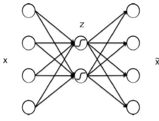
Autoencoder is an unsupervised machine learning technique. Basically, it is a neural network that is trained to attempt to replicate its input to its output. Internally, it has hidden layers which describe the representation of the input data. The network may be viewed as consisting of two parts. Encoder and decoder. The basic structure of an autoencoder is shown in the fig.2.2.

Figure 2.2: Basic structure of Autoencoder

Let x be the input with data points{x1, x2, ..., xm}, where each data point has many dimensions. The encoder is the one which transforms these input to lower dimension data z. Let the data points in the reduced dimension be{z1, z2, ..., zm}. The decoder is the one tries to reconstruct high dimensional data. Decoded output be ˜x with data points{x˜1_,_x_˜2_{, ...,}_x_˜m_}_{. So encoder maps data} {xi_}_{to compressed data} _{_zi_}_{and decoder maps compressed data}_{_zi_}_{back to} _{_x_˜i_}_.

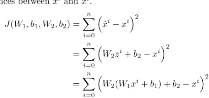
Formulating ˜xand zas a function of their input we have

zi=W1xi+b1 ˜

xi=W2xi+b2

(14)

sum of squared differences between ˜xi _and_xi_. J(W1, b1, W2, b2) = n X i=0 ˜ xi−xi 2 = n X i=0 W2zi+b2−xi 2 = n X i=0 W2(W1xi+b1) +b2−xi 2

This is minimized using stochastic gradient descent. Above equations represent a linear relation. Hence it is a linear autoencoder. If our data points are coming from a nonlinear surface then we should go for non-linear autoencoders which will have non-linear activations. If we use more hidden layers then it become a deep autoencoder model.

2.3

Support Vector Regression (SVR)

When a support vector machine applied to a regression problem then it is termed as Support Vector Regression (SVR). When we use SVM for a two-class classification problem, actually what it tries to do is to find a hyperplane that best separates two classes with a minimum error while also making sure that the perpendicular distance between the two close points from either of these two classes is maximized. This is the mode of determination of hyperplane separating classes. For the above case, determination of hyperplane set with the constraints

~

w·x~i−b≥1if yi= 1

or

~

w·x~i−b≤ −1if yi=−1

The visualization looks similar to fig.2.3.

Figure 2.3: 2 class classification problem using SVM

SVR is not a classification problem but a regression problem. Here also we require a hyperplane with points on both sides of it along with the constraint that distance between these points and the line should not farther than epsilon. That is,

(15)

wxi+b−yi≤

Instead of minimizing the observed training error, Support Vector Regression (SVR) attempts to minimize the generalization error bound so as to achieve generalized performance. The idea of SVR is based on the computation of a linear regression function in a high dimensional feature space where the input data are mapped via a non-linear function.

2.4

Generative Adversarial Networks

Generative Adversarial Networks or GANs is an unsupervised technique introduced in 2014 by Goodfellow et al. [1]. A GAN consists of two models: Generator and Discriminator. One is a counterfeiter trying to produce seemingly real data while the other one trying to determine fake counterfeit data also taking care for not raising false positives on real data. The generative model takes some random input and tries to generate samples that resembles real data. It has no idea of what is the real data, it will only try to adjust from the feedback of the other model. The discriminative model will take a bunch of generated data from the other model and actual real data as input.

(a) Overview of GAN. (b) Training of GAN.

Training of GAN consists of two steps: training of discriminator and training of generator via chained models. Training of the discriminator is done by sampling some images from the dataset and some noise that will pipe through the generator model. Then use this data to train the discriminator to recognize generator data from real data. In training the generator via the chained models, we will first generate sample data and try to push the chained generator and discriminator to tell that it is real data. However, we will not alter the weights in the discriminator during this step. It is achieved by freezing the training of the weights in the discriminator. Not only as a purpose of generating images, GAN proved its importance in the field of super resolution, de-noising and de-blurring [2]. Image to image translation also performs well using GAN [3]

2.4.1

Related work

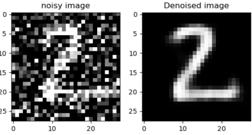
As an initial work, a denoising autoencoder is tried among MNIST database. To each training sample in MNIST database added a random noise and trained the autoencoder network with noisy and corresponding noiseless images. Fig.4.3 shows the result.

(16)

Figure 2.5: Denoised image from MNIST database

As an initial step for the generative model, I generated digits by testing the model described in [4]. The results are shown in figs.(a)-(i).

The network consists of generator and discriminator. The generator is a network which tries to generate a 28×28 digit image from a noisy input. The discriminator is a deep convolutional neural neural networks which perform classification between real and fake images. While training the discriminator it is fed with the fake data generated from the generator along with the images in the MNIST database [5].

(17)

(a) After 1000 iterations. (b) After 2000 iterations. (c) After 3000 iterations.

(d) After 5000 iterations. (e) After 6000 iterations. (f) After 7000 iterations.

(18)

Chapter 3

Literature Survey

Image processing is a rapidly evolving field with immense significance in science and engineering where image quality assessment is a significant area of research [6]. The main tools used for calcu-lating the quality were the Mean Squared Error (MSE) and Peak Signal to Noise Ratio (PSNR). But they didn’t well correlate with human subjective scores [7]. Sheikhet al. [8] conducted a study on the evaluation of full reference IQA algorithms which gives the way to think of the factors which going to affect the quality of the image. K.Seshadrinathan et al. [9] conducted a similar study on videos. This also provides directions for designing better algorithms which can come up with an image quality that will highly be correlated with the subjective scores.

The invention of the Structural Similarity Index (SSIM) by Wang et al. [10] gives a drastic change in the area of quality assessment. This algorithm shows that structure is a predominant factor in the determination of the quality. It considers three factors for calculating quality, which includes luminance, contrast, and structure. A comparison with existing MSE measures also proves the importance of structure for quality assessment [11]. This is one of the dominant algorithms for FRIQA. Later Zanget al. extended the concept of SSIM to MSSSIM [12] by considering the images at different scales with the incorporation of filter bank concept. This results in an the improvement in the assessment. Zhang et al. proposed the Feature similarity index (FSIM) for image quality assessment [13] which considers phase congruency and gradient magnitude as the primary features for calculating quality. While all the previous algorithms including SSIM and MSSSIM consider all images patches with equal importance, FSIM gives importance to the phase of each patch. It deals with the idea that the patches with higher phase congruency can extract more features. Sheikhet al. gives importance to the idea of image information fidelity [14]. This algorithm deals with the amount of information extracted by the brain from the reference images, the loss of this information is quantified as the distortion.

All the above metrics represent full reference quality assessment algorithms. But in many prac-tical cases we will not be provided with the pristine version of the distorted image. This gives the way for researchers to look more into the problems of no reference quality assessment algorithms. Most of the predominant algorithms in the literature first try to learn statistics of the image using different tools and then obtained features are correlated with the human subjective scores. Saad et al. [15] looked at the changes in the statistical features of the distorted image from the pristine, and used these features to train a statistical model completely in the DCT framework. Mittal et al. [16] introduced blind/reference less image spatial quality evaluator (BRISQUE) which uses scene statistics of locally normalized luminance coefficients to quantify possible losses of naturalness in the image due to the presence of distortions. This method doesn’t use any transformation to other domain like DCT domain transformation used in [15]. Moorthy et al. in his work [17] viewed the problem in a different way by finding the distortion first followed by the distortion specific qual-ity assessment. This work is also based on natural scene statistics which governs the behaviour of natural images. Later researches start looking at the dictionaries for sparse representation [18] for image quality assessment. Priya et al. constructed an overcomplete dictionary using pristine images by utilizing the K-SVD algorithm [19] and presented alteration in the sparse representation

(19)

of natural images in the presence of distortions [20]. Sparse representation of set of pristine images are extracted initially, and quality is found by calculating the sparse representation of a given image and quantified with respect to reference features. The similar idea is extended to the work along with the modelling of Univariate Generalized Gaussian Distribution (UGGD[21]). They showed that modelling UGGD parameters will give better features for distortion discrimination. The completely blind work proposed by Mittalet al. [22] made a drastic change in the research of no reference image quality assessment, which is the first opinion unaware distortion unaware NR IQA algorithm in the literature. It is based on the extraction of quality aware features and fitting them to a multivariate Gaussian (MVG) model. Quality is estimated by calculating the distance between the MVG fit of the NSS features extracted from the test image and an MVG model of the quality-aware features extracted from the corpus of natural images.

All algorithm presented above are image quality assessment algorithms. There also many promi-nent works in the video quality assessment area also. In video cases also researchers started by looking at the statistics of the natural videos and finding how much the statistics got disturbed in distorted videos. Seshadrinathan et al. developed full reference video quality assessment algo-rithm [9] for measuring both spatial and temporal video distortions over multiple scales, and along motion trajectories, while accounting for spatial and temporal perceptual masking effects. They utilized Gabor filters for extracting features. Wang et al extended the idea of SSIM in the tem-poral direction and applied to videos in [23]. Mittal et al. developed VIIDEO [24], a no reference video quality assessment algorithm which observed the statistical regularities of natural videos and quantified disturbances introduced due to distortions. Manasa.et al. looked at the optical flow characteristics of the videos in [25] and suggested the idea that local optical flow statistics are af-fected by distortions and the deviation from pristine flow statistics is proportional to the amount of distortion. Shabeeret al. in [26] extended the idea of sparse representation of images to videos for quality assessment. They constructed spatio-temporal dictionaries for videos using the K-SVD algorithm [19]. They used Generalized Gaussian Distribution (GGD) to model the sparse represen-tation of each atom of the dictionary and showed that these GGD parameters are well suited for distortion discrimination.

Entry of Deep learning [27] made a drastic change in the field of image processing and qual-ity assessment. Initially researches started to look into basic classification problems using deep networks [28]. By the introduction of autoencoders, convolutional neural networks and recurrent neural networks [29] the research area become more and more strong. Autoencoders are unsuper-vised neural networks and can be used as a generative model aswell. They are able to give good lower dimensional representation for the input data. Automatic learning of the features became possible by the arrival of convolutional neural networks. Since convolutional neural networks consider input data points to be independent, the CNN models fail to perform in data points that are having time dependencies. For exploiting time dependencies we should need all data points and following hid-den layers should be connected to the preceding once which paved the way for the invention of the Recurrent Neural Networks (RNN). Gielet al. used RNNs for action recognition in videos [30] by exploiting transfer learning. Video processing becomes much easier by the entry of RNN but there were also problems because of vanishing gradient and long-term dependency among data points. This problem is solved by Long Short Term Memory (LSTM) networks [31, 32]. The basic units of LSTMs are cells which have more features including addition and removal of features to cell state. They have additive interaction between cell states which resolves the problems of vanishing gradi-ents. Long-term Recurrent Convolutional Networks (LRCN) are the combination of both CNNs and LSTMs. Donahueet al. used LRCN for visual recognition in [33]. The developed network is also capable of giving a description of the result.

Deep learning has also made a notable impact in the field of image quality assessment. The idea of using deep neural networks for extracting quality features is slightly inspired by the CORNIA [34] work where they extracted quality features by filter learning. Kanget al. used convolutional neural network framework for no reference image quality assessment in [35]. They proposed a simple network consisting of one convolution layer, one min and one max pooling layer and finally a fully connected layer. It overperformed over all the statistical methods of that time. Seyedet al. proposed a full reference image quality algorithm [36] by looking at the features after each convolution layer.

(20)

Features are extracted from a pre-trained Alexnet model. They compared feature maps of pristine and distorted image at each layer and pooled them for obtaining the quality score. Zhanget al in [37] showed that semantic analysis is also crucial in quality evaluation along with the signal-space analysis. Their network consists of two parts, one for extracting local characteristics and other for the evaluation of semantic obviousness and final quality is estimated by fusing these two features. Bosseet al. used a similar idea in [35] but extended the network to a more deeper one. They also proposed a full reference algorithm [38]. In the full reference case, they trained two different neural networks separately and merged them using a concatenation layer. They also trained fully connected layers in parallel with the regression part to get weights of each patch of the image. Researchers are exploring more in deep learning methods for inventing new analysis tools in image quality assessment.

(21)

Chapter 4

Autoencoder based Full reference

Previous literature shows that statistical features of pristine images will get modified in the presence of distortion. Algorithms using deep learning do well at extracting quality features. This gave the inspiration to explore features from deep neural networks and checking how they are affected in the presence of distortion. Since image dimensions are typically large to explore, lower dimensional representation of the pristine image and finding the changes in their representation in presence of distortion. The model which can give a good lower dimensional representation is an autoencoder.

4.1

Proposed method

In this work, I implemented a full reference image quality algorithm in an unsupervised manner. Since it is completely unsupervised, I have not used any labels. I have used an autoencoder for this task. An autoencoder is a convolutional neural network consisting of encoder and decoder. Autoen-coder tries to replicate the input exactly at the output after going through a stage of dimensionality reduction. The decoder part of the autoencoder should be efficient and should be able to generate a high dimensional data from the low dimensional data. Encoded features are extracted for pristine distorted image and their difference is found using different metrics. These distance measures are correlated with subjective scores. I will explain each step in the following sections.

4.1.1

Feature Extraction

Since it is an unsupervised approach I dont use any training labels but instead try to reconstruct in-put exactly at the outin-put. Only pristine image patches from the Waterloo Exploration database [39] are used for training.Different patch sizes considered in this work includes 256×256, 128×128 and 64×64. Autoencoder model tried best to replicate input exactly at the output. Input and decoded results for some test images are shown in the fig.4.1.

(22)

Figure 4.1: Input image and decoded Image

Network Architecture for Autoencoder

Since the purpose of training is to reduce the difference in input and decoded image, mean squared error is considered as the loss function. Network architecture for autoencoder is shown in the table 5.1. The encoder network consists of certain convolution layers followed by maxpooling layers and the decoder network consist of convolution layers followed by upsampling layers. The number of parameters of each layer is shown in the table 5.1. The encoder output has a much-reduced dimension compared to the input but the dimension of decoded result and input are the same.

Table 4.1: Autoencoder network architecture

Layer(Type) Output shape Parameters

input 1(InputLayer) (None,256,256,3) 0

conv2d 1(Conv2D) (None,256,256,16) 448

max pooling2d 1(MaxPooling2D) (None,128,128,16) 0

conv2d 2(Conv2D) (None,128,128,8) 11160

conv2d 3(Conv2D) (None,64,64,8) 584

up samplind2d 1(UpSampling2D) (None,64,64,8) 0

conv2d 6(Conv2D) (None,128,128,16) 1168

conv2d 7(Conv2D) (None,256,256,3) 435

4.1.2

Quality Measurement

Encoded output features are taken for calculating the quality. They are the lower dimensional representation of the given input. Since it is a full reference method, I have distorted image and corresponding pristine image is available at the input. Let R and D represents input real (pristine) and distorted images respectively. R’ and D’ represent decoded pristine and distorted images. fd

andfrrepresent encoded feature vector of pristine and distorted image. The difference between the

encoded feature vector of both pristine and distorted input is calculated. Several distance measures are considered for calculating the distance. The distance measures considered in this work are represented as follows,

(23)

Distance measures

Letfrandfdbe two vectors of lengthNrepresenting the encoded output of the pristine and reference

• City block Distance:

DCb(fr, fd) = N X i=1 |fri−fdi| • Gower Distance: DGow(fr, fd) = 1 N N X i=1 |fri−fdi|

This distance measure betweenfrandfd used for quality estimation denoted byq.

4.1.3

Finding Correlation

Next step is evaluate the performance of the above metric. For that purpose I find how well the ’q’ scores are correlated with subjective scores. Most of the database provide DMOS as the subjective scores. DMOS represents the differential mean opinion scores. Higher the DMOS scores imply lower the quality. Linear Constant Correlation (LCC) and Spearman Rank Order Correlation Co-efficient (SROCC) are found between q scores and DMOS values. The algorithm is looked in a supervised way also by training an SVR. 80:20 split is used for train and validation while training. Different kernels in SVR also tried.

4.2

Results and Discussion

4.2.1

Datasets

Autoencoder is trained only using the pristine images from the Waterloo database. Testing of the model is performed on the remaining datasets mentioned in the table.

(24)

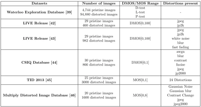
Table 4.2: Datasets

Datasets Number of images DMOS/MOS Range Distortions present Waterloo Exploration Database [39] 4,744 pristine images

94,880 distorted images

D-test L-test P-test

-LIVE Release [42] 29 pristine images

460 distorted images DMOS[0,100]

jpeg jp2k

LIVE Release [43] 29 pristine images

jpeg jp2k white noise

blur fast fading

CSIQ Database [44] 30 pristine images

awgn blur contrast fnoise jpeg jp2000

TID 2013 [45] 25 pristine images

3000 distorted images MOS[0,1] 24 Distortions

Multiply Distorted Image Database [46] 20 pristine images

1600 distorted images MOS[0,8]

Gaussian Noise Gaussian blur Contrast Change jpeg jpeg2000

4.2.2

Performance evaluation

There are three different models for each patch size. Different distance features are extracted from each model. These features are calculated separately for each distortion in the LIVE database. Dis-tance features are calculated by measuring the error between encoded features of pristine and dis-torted images. Encoded results fr0m the model is taken and it is transformed into a one-dimensional vector and then calculated the distance using the measures presented in the section 5.12. The graph showing the relation between the absolute error distance features and the subjective scores is represented in the fig.5.2.

Figure 4.2: Scatter plot showing the relation between subjective scores and absolute error between encoded features of the pristine and distorted image.

Correlation is found separately for different distortions present in LIVE Release2 database for the model which trained with a patch size of 64×64. Obtained results are presented in the table.5.3].

(25)

Table 4.3: Comparison of the performance of the model trained with patch size 64×64 over different distortion types in LIVE Realease2

Distance/

Distortions Jp2k Jpeg Wn Gblur Ffading All

Euclidean 0.7575 0.7870 0.8048 0.7810 0.6625 0.5440 Gower 0.7430 0.7732 0.8083 0.7095 0.6421 0.5159 Chebyshev 0.7498 0.8018 0.8190 0.7942 0.6729 0.6223 Soergel 0.7676 0.7830 0.8260 0.7238 0.6602 0.5424 Sorensen 0.7638 0.7782 0.8088 0.7185 0.6541 0.5226 Kulczynski 0.7598 0.7732 0.7876 0.7125 0.6472 0.4994 City block 0.7430 0.7732 0.8083 0.7095 0.6421 0.5159 Lorentzian 0.7481 0.7782 0.8625 0.7127 0.6491 0.5321

The second trained model is the one with the patch size of 128×128. This model is tested against all the distortions present in the LIVE release database. There are five distortions present in the database. Overall correlation values are also presented in the table 5.4.

Table 4.4: Comparison of the performance of the model trained with patch size 128×128 over different distortion types in LIVE Release2 database

Distance/

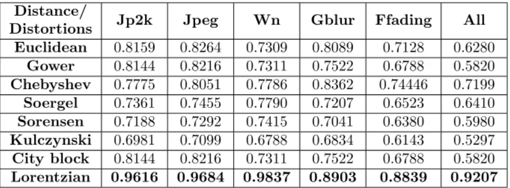
The third trained model is the one with the patch size of 256×256. This model is tested against all the distortions present in the LIVE database release2. The correlations are noted in the table 5.5.

Apart from taking the encoded vector as the feature, decoded features are also considered. The same procedure followed for encoded features is repeated for decoded features also. Decoded results are the one which preserves the same shape as the that of the input image. Decoded result is taken for both pristine and distorted images. It is vectorized and the distance between these two vectors is found using different distance metrics. The scatter plot showing the relation between absolute distance between decoded reference and decoded distorted image and corresponding subjective scores for the images present in the LIVE database is shown in the fig.5.3.

The decoded result is taken from the model which trained using the patch size of 256×256 for all the images of the LIVE database. Different distance measures are calculated between the decoded reference image and the decoded distorted image. Correlation scores between these distance features and subjective scores for all distortions in the LIVE database is shown in table 5.6.

Next method considered in a supervised manner. The encoded distance measures which is highly correlated with the human subjective scores are taken as the input feature to a support vector regression(SVR) and trained it against the DMOS values. The distance features considered are the Lorentzian distance and Chebyshev distance. The testing is performed on the model which is trained for the patch size of 256×256. Results are presented in the table 5.7.

(26)

Table 4.5: Comparison of the performance of the model trained with patch size 256×256 over different distortion types in LIVE Realease2 databse

Distance/

Figure 4.3: Scatter plot showing the relation between subjective scores and the absolute error between the decoded features of the pristine and distorted image

The same procedure is repeated for other standard databases for image quality assessment which are listed in the table 5.2. Encoded features are taken in to consideration for training the SVR. Testing for the images of LIVE database is performed among all the three models. For all other datasets model which taken into consideration is the one which trained with the patch size of 256×256.

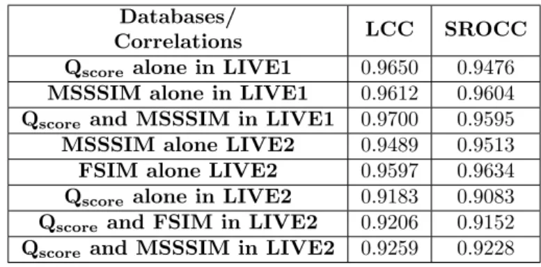
One more method which I tried is the training along with existing full reference metrics. Feature Similarity Metric (FSIM) and Multi Scale Structural Similarity Index Metric (MSSSIM) are two powerful full reference metrics in the literature. These are the metrics with state of the art perfor-mance. Along with the distance MSSSIM is also considered for training the SVR. Another one is by considering FSIM feature along with the distance metric. Same encoded distance features taken in the previous cases are considered here also. The model considered is the one which trained with the patch size of 256×256. The corresponding correlations obtained while testing are listed in the table 5.9.

4.3

Conclusion

We presented a full reference image quality assessment algorithm using Autoencoders. It is a com-pletely unsupervised method. The key features of this method is taking the features from a trained

(27)

Table 4.6: Comparison of the performance of the model train with patch size 256×256 using decoded result as the feature over different distortion types on the LIVE Release2 database

Distance/

Distortions Jp2k Jpeg Wn Gblur Ffading

Euclidean 0.8227 0.8007 0.7203 0.8088 0.7041 Gower 0.8003 0.7794 0.7025 0.7337 0.6622 Chebyshev 0.8254 0.8131 0.8418 0.8569 0.7782 Soergel 0.6957 0.7094 0.6864 0.6938 6246 Sorensen 0.6878 0.7017 0.6477 0.6865 0.6160 Kulczynski 0.6792 0.6918 0.5863 0.6783 0.6061 City block 0.8003 0.7794 0.7025 0.7337 0.6622 Lorentzian 0.8047 0.7831 0.7152 0.7396 0.6693

Table 4.7: Comparison among differnt distortions training SVR

Correlations/

LCC 0.9599 0.9652 0.9855 0.8669 0.8756 0.9183

SROCC 0.9594 0.9457 0.9864 0.8825 0.8841 0.9190

autoencoder. A deep convolutional autoencoder is trained only using the pristine images from Wa-terloo exploration database. Three different models are trained with patch sizes 64×64, 128×128 and 256×256. Different distance features are evaluated between encoded features of distorted and reference images. It is found that these distance features are highly correlated with human subjec-tive scores. It is also observed that correlation values are improving with size of the patch. For low patch sizes Chebyshev distance features shows better correlation with DMOS but as the patch size increases the Lorentzian distance features are the onee with high correlation values. Testing is performed with decoded features also but better result is obtained with encoded features. The same algorithm is extended in a supervised way by training an SVR. The input features to the SVR is distance feature which gives high correlation with subjective scores. It is trained against the DMOS scores. Performance of the algorithm is improved using the supervised technique. Along with encoded distance features existing FR IQA metrics also used for training the regression. the performance of the algorithm is therefor boosted in this case.

(28)

Table 4.8: Comparison among different datasets Correlations/ Distortions LCC SROCC Live Release1 0.9650 0.9476 Live Release2 64 0.8551 0.8546 Live Release1 128 0.8758 0.8352 Live Release1 256 0.9183 0.9190

Live Multi distortion 0.6815 0.6725

CSIQ 0.7359 0.7299

Table 4.9: Comparison among different sets by MSSSIM and FSIM as one feartures.

Databases/

Correlations LCC SROCC

Qscore alone in LIVE1 0.9650 0.9476

MSSSIM alone in LIVE1 0.9612 0.9604

Qscore and MSSSIM in LIVE1 0.9700 0.9595

MSSSIM alone LIVE2 0.9489 0.9513

FSIM alone LIVE2 0.9597 0.9634

Qscore alone in LIVE2 0.9183 0.9083

Qscore and FSIM in LIVE2 0.9206 0.9152

(29)

Chapter 5

CNN based Full Reference and No

Reference Image Quality

Assessment

Deep convolutional neural networks is good at extracting features for several computer vision tasks. Automated feature extraction that helps to differentiate the distortions from their pristine images would be useful for IQA. If we are giving both reference and distorted image to a deep model and the model lerns to give quality scores it would reduce the load of extracting features and doing post-processing. In all previous methods, we should ourself look at those features which can perform efficiently. This gives the motivation to look into more deeper networks. Existing literature shows that using deep networks helps in improving performance. This leads me the way to propose a deep convolutional neural network based full reference and no reference image quality assessment.

5.1

Proposed Method

In this work, I predicted image quality in a supervised manner. Here I tried the algorithm in both full reference and no reference case seperately. I tried replicating the work in [38].

5.1.1

Full reference image quality assessment

Here I trained a convolutional neural network with both pristine and distorted image as input and corresponding DMOS score as the label. For training, I used LIVE database Release 2 [43]. The block diagram of the work is represented in fig.6.1. There are two similar deep Convolutional

Figure 5.1: Block diagram of the FRIQA algorithm

Neural Network (CNN) architectures which get trained separately. The CNN extracts features from distorted and reference image patches and estimates the perceived quality of the distorted image by combining the features and training a regression using two fully connected layers. The overall IQA

(30)

score is computed by aggregating the patch quality estimates. fr andfd are the features obtained

after deep convolutional layers from pristine and distorted images respectively. These features are concatenated using a concatenation layer for performing the regression. 64 × 64 RGB patches are cropped from the reference and the distorted images. Patches are assigned with the quality labels given to the full image from where the respective patch are cropped. Features are fused by concatenatingfr, fd andfr−fd

Fused feature vectors are given as input to a fully connected neural network for performing regression to get a patch quality estimate. Patch quality estimates are aggregated to an image quality estimate. Training is performed by minimizing the mean absolute error (MAE). Two additional fully connected layers are added in parallel with fully connected layers for regression to get the weighted average aggregation of patch wise estimated local quality to global quality in the work [47].

5.1.2

No reference image quality assessment

No reference image quality assessment algorithm is implemented in a similar way as in the case of the full reference method. The network has only one input, which is the patch taken from the input image. A given patch will pass through certain convolutional layers to extract the features. The network is trained in such a way that for a given a test image it will be able to give image quality. Block diagram of the no refernce work is represented in the figure[6.2].

Figure 5.2: Block diagram of NRIQA algorithm

5.1.3

Network Architecture

In all convolutional layers initial layers will be able to extract low-level features and as the network goes deeper the final convolutional layers will be able to extract high-level features. The network is deep consisting of eight convolutional layers with max pooling layers after two convolutional layers. In full reference work consist of extra merging layer to concatenate different features obtained after convolutional layer. Passing reference and distorted patch separately through different convolutional layers and concatenate the features is actually inspired by a stereo work [48]. Two fully connected layers are used at the end for performing regression, i.e, to get image quality from patch quality. The network architecture for the full reference work is described in the table 7.1.

5.1.4

Quality Estimation

Image quality is calculated by taking the average patch quality estimates. LetNpbe the number of

patches taken from a image andyi be the patch quality estimate for a given patch i. Image quality

is given by q= PNp i yi Np .

5.2

Results and Discussions

Reference images from LIVE [43] and TID2013 [45] database are divided into two for testing and training. 19 reference image and associated distorted images are used for training and remaining are used for testing. Separate models are trained for each databases. The algorithm is evaluated on the test images of the same dataset.

(31)

Table 5.1: Full reference network architecture

Layer(Type) Output shape Parameters Connected to

input 1 1(InputLayer) (None,64,64,3) 0 -input 2 2(InputLayer) (None,64,64,3) 0 -block1 conv1 1(Conv2D) (None,64,64,64) 1792 input 1 1 block1 conv1 2(Conv2D) (None,64,64,64) 1792 input 2 2 block1 conv2 1(Conv2D) (None,64,64,64) 36928 block1 conv1 1 block1 conv2 2(Conv2D) (None,64,64,64) 36928 block1 conv1 2 block1 pool 1(MaxPooling2D) (None,32,32,64) 0 block1 conv2 1 block1 pool 2(MaxPooling2D) (None,32,32,64) 0 block1 conv2 2 block2 conv1 1(Conv2D) (None,32,32,128) 73856 block1 pool 1 block2 conv1 2(Conv2D) (None,32,32,128) 73856 block1 pool 2 block2 conv2 1(Conv2D) (None,32,32,128) 147584 block2 conv1 1 block2 conv2 2(Conv2D) (None,32,32,128) 147584 block2 conv1 2 block2 pool 1(MaxPooling2D) (None,16,16,128) 0 block2 conv2 1 block2 pool 2(MaxPooling2D) (None,16,16,128) 0 block2 conv2 2 block3 conv1 1(Conv2D) (None,16,16,256) 295168 block2 pool 1 block3 conv1 2(Conv2D) (None,16,16,256) 298168 block2 pool 2 block3 conv2 1(Conv2D) (None,16,16,256) 590080 block3 conv1 1 block3 conv2 2(Conv2D) (None,16,16,256) 590080 block3 conv1 2 block3 conv3 1(Conv2D) (None,16,16,256) 590080 block3 conv2 1 block3 conv3 2(Conv2D) (None,16,16,256) 590080 block3 conv2 2 block3 pool 1(MaxPooling2D) (None,8,8,256) 0 block3 conv3 1 block3 pool 2(MaxPooling2D) (None,8,8,256) 0 block3 conv3 2 block4 conv1 1(Conv2D) (None,8,8,512) 1180160 block3 pool 1 block4 conv1 2(Conv2D) (None,8,8,512) 1180160 block3 pool 2 block4 conv2 1(Conv2D) (None,8,8,512) 2359808 block4 conv1 1 block4 conv2 2(Conv2D) (None,8,8,512) 2359808 block4 conv1 2 block4 conv3 1(Conv2D) (None,8,8,512) 2359808 block4 conv2 1 block4 conv3 2(Conv2D) (None,8,8,512) 2359808 block4 conv2 2 block4 pool 1(MaxPooling2D) (None,4,4,512) 0 block4 conv3 1 block4 pool 2(MaxPooling2D) (None,4,4,512) 0 block4 conv3 2 block5 conv1 1(Conv2D) (None,4,4,512) 2359808 block4 pool 1 block5 conv1 2(Conv2D) (None,4,4,512) 2359808 block4 pool 2 block5 conv2 1(Conv2D) (None,4,4,512) 2359808 block5 conv1 1 block5 conv2 2(Conv2D) (None,4,4,512) 2359808 block5 conv1 2 block5 conv3 1(Conv2D) (None,4,4,512) 2359808 block5 conv2 1 block5 conv3 2(Conv2D) (None,4,4,512) 2359808 block5 conv2 2 block5 pool 1(MaxPooling2D) (None,2,2,512) 0 block5 conv3 1 block5 pool 2(MaxPooling2D) (None,2,2,512) 0 block5 conv3 2 flatten 1(Flatten) (None,2048) 0 block5 pool 1 flatten 2(Flatten) (None,2048) 0 block5 pool 2 subtract 1(Subtract) (None,2048) 0 flatten 1 , flatten 2 concatenate 1(Concatenate) (None,6144) 0 flatten 1 , flatten 2 , subtract 1

dense 1(Dense) (None,4096) 25169920 concatenate 1 dense 2(Dense) (None,2048) 8390656 dense 1 dense 3(Dense) (None,1) 2049 dense 2

Cross-dataset validation

Here I trained my model on full LIVE release2 database and tested on CSIQ [44] and TID 2013. Testing is done on the full dataset as well as their subsets. Subset means testing it contains only for distortions common with the training set. Both the CSIQ and TID2013 datasets share only four distortions in common with the LIVE database. The correlations obtained are presented in the table 6.3.

5.3

Conclusion

We proposed a full reference and no reference image quality algorithm using deep convolutional neural networks. Learning is done in a supervised manner. For the full reference case, the metric is able to give quality scores if it is provided with the test image and its corresponding reference image. If the test image is input to the no reference metric it will give the quality score. The algorithm is

(32)

Table 5.2: Performance evaluation

Datasets/Metrics LIVE TID2013

LCC SROCC LCC SROCC

Full reference 0.9777 0.9662 0.8808 0.8591

No reference 0.9120 0.9001 0.8552 0.8354

Table 5.3: Cross dataset evaluation

Metrics/Datasets Full reference No reference

LCC SROCC LCC SROCC

CSIQ subset 0.8722 0.8661 0.9085 0.8808

CSIQ 0.7046 0.6602 0.6927 0.6811

TID2013 subset 0.8719 0.8517 0.8627 0.8487

TID2013 0.4327 0.4115 0.3924 0.3625

performing efficiently and is able to give quality values which are highly correlated with the human subjective scores. the algorithm is performing better if the learned model is trained with more types of distorted images.

(33)

Chapter 6

Classification based No Reference

Researchers are dealing with mostly regression problems for assessing image quality. For assessing local features we consider small patch sizes. Distortion level may vary from one region to another region within an image i.e, we may not be able to view distortion in some parts of an image but it may be present in other parts. For a highly distorted image, most of the patches in it will be of low quality. But for undistorted image most of the patches will be of high quality. The case is different for an image having a medium level of distortion where we can find some patches with low quality and some with high quality. This gives me the thought of looking into a classification model which can classify a given input patch into low quality or high quality. But the model should be trained for very low patch size so that it can extract the local features.

6.1

Proposed Method

In this work, we propose an unsupervised technique for no reference image quality assessment using classification. Mostly IQA algorithms using deep learning operate in the regression network. But in our proposed method, the primary network is a classifier which is able to classify the images based on the quality. A simplest schematic representation of the classifier is depicted in the fig.7.1.

Figure 6.1: Block diagram for classification.

Initially, we trained a classification network which is able to classify a given input patch is having high quality or low quality. The input to the network consists of high quality and low quality image patches with high quality patches assigned with a label 1 and low quality patches assigned with a label 0.

We also viewed the problem as a multi-class classification problem in which instead of training a two-class classification network I trained a multi-class classifier. In this framework, each class represents a type of distortion along with one extra class which representing the pristine images. If the given patch is high-quality then high quality class will be assigned with a label 1 and remaining all distortion classes will be assigned with a label 0. If the given patch is of low quality the corresponding distortion class label will be assigned label 1 and all remaining classes will be assigned 0.

(34)

The images taken for training depend on the datasets and the level of distortion present. In general, I considered pristine images to be the ones with high quality and those with a high DMOS score are the one with a higher level of distortion and considered to be low quality. Only highly distorted image and pristine images are considered for training.

6.1.1

Network Architecture

Our network consists of six convolution layers, three maxpooling layers and finally, we have a fully connected layer at the end with softmax as the activation function. Each convolution layer is defined with an activation of Relu. The loss function defined for classification is categorical cross entropy. For a two class classification problem, there are two nodes at last fully connected node and in a multi-class classification the number of nodes at last fully connected layer equal to the number of distortions plus one (One extra node for pristine). The network architecture is described in the table 7.1.

Pre-trained VGG16 model is also used with initial few layers fused and by adding two fully connected layers at the end.

Table 6.1: Classifier network architecture

Layer(Type) Output shape Parameters

input 1(InputLayer) (None,32,32,3) 0

conv2d 2(Conv2D) (None,32,32,32) 896

batch normalization 1

(BatchNormalization) (None,32,32,32) 128

dropout 1(Dropout) (None,16,16,32) 0

conv2d 3(Conv2D) (None,16.16.64) 18495

conv2d 4(Conv2D) (None,16,16,64) 36928

dropout 2(Dropout) (None,8,8,64) 0

conv2d 5(Conv2D) (None,8,8,64) 36928

conv2d 6(Conv2D) (None,8,8,64) 36928

flatten 3(Flatten) (None,1024) 0

dense 1(Dense) (None,1024) 1049600

dense 2(Dense) (None,2) 2050

6.1.2

Quality Measurement

A given image is divided into the number of patches and given to the classification network. Once the classification is performed, each given input patch will be assigned with a label 1 or 0. The next step is to find the image quality from patch labels. From the patch labels, image quality score for a given image is obtained by taking the average of labels of all patches available in a given image. Let

(35)

the quality scoreQfor an image is obtained by the formula. Q= 1 Np Np X i=1 qi.

In multi-class classification problem also the image quality score is obtained by taking the average of the labels of all high-quality class among all patches.

6.2

Results and Discussions

Images from LIVE database is used for training and testing is performed on CSIQ and TID2013 databases. There are septate models for patch size of 32×32 and 64×64. Fig.7.1 represent the loss versus epoch diagram and accuracy versus epoch diagram respectively. Both training and validation loss are plotted in the figure.

(a) Model accuracy v/s epoch (b) Model loss v/s epoch

The correlation obtained while testing the classifier model which rained on LIVE database is represented in the table 7.2.

Table 6.2: Comparison among different patch sizes for the model trained on LIVE

Datasets/Patch size CSIQ TID2013

LCC SROCC LCC SROCC

32 ×32 0.5538 0.5390 0.2955 0.2924

64 ×64 0.6248 0.6135 0.3897 0.3612

Two more models are trained for same patch sizes but using the TID2013 database. Result of the comparison among different datasets is represented in the table 7.3.

Table 6.3: Comparison among differnt patch sizes for the model trained on TID2013

Datasets/Patch size CSIQ LIVE Release2

LCC SROCC LCC SROCC

32 ×32 0.6127 0.6020 0.6484 0.6383

64 ×64 0.6689 0.6601 0.7012 0.6892

6.3

Conclusions

We proposed a no reference image quality algorithm using classification as the basic framework. A given test image is divided into a number of patches and each patch is classified into high quality or

(36)

low quality by the classification network. Quality is calculated by taking the average of the patch labels. The algorithm is efficient to give quality scores which are having a high correlation with subjective scores. It is observed that better results are obtained with higher size patches. The algorithm is performs more efficiently if the classification model is trained with a higher number of distortions.

(37)

References

[1] I. J. Goodfellow. NIPS 2016 Tutorial: Generative Adversarial Networks.CoRRabs/1701.00160. [2] Q. Yan and W. Wang. DCGANs for image super-resolution, denoising and debluring. 2017 . [3] P. Isola, J. Zhu, T. Zhou, and A. A. Efros. Image-to-Image Translation with Conditional

Adversarial Networks. CoRRabs/1611.07004.

[4] A. Radford, L. Metz, and S. Chintala. Unsupervised Representation Learning with Deep Con-volutional Generative Adversarial Networks. CoRR abs/1511.06434.

[5] Y. LeCun and C. Cortes. MNIST handwritten digit database .

[6] Z. Wang, A. C. Bovik, and L. Lu. Why is image quality assessment so difficult? In 2002 IEEE International Conference on Acoustics, Speech, and Signal Processing, volume 4. 2002 IV–3313–IV–3316.

[7] B. Girod. Psychovisual Aspects Of Image Processing: What’s Wrong With Mean Squared Error? In Proceedings of the Seventh Workshop on Multidimensional Signal Processing. 1991 P.2–P.2.

[8] H. R. Sheikh, M. F. Sabir, and A. C. Bovik. A Statistical Evaluation of Recent Full Reference Image Quality Assessment Algorithms. IEEE Transactions on Image Processing 15, (2006) 3440–3451.

[9] K. Seshadrinathan and A. C. Bovik. Motion Tuned Spatio-Temporal Quality Assessment of Natural Videos. IEEE Transactions on Image Processing 19, (2010) 335–350.

[10] Z. Wang, A. C. Bovik, H. R. Sheikh, and E. P. Simoncelli. Image quality assessment: from error visibility to structural similarity. IEEE Transactions on Image Processing 13, (2004) 600–612. [11] Z. Wang and A. C. Bovik. Mean squared error: Love it or leave it? A new look at Signal

Fidelity Measures. IEEE Signal Processing Magazine 26, (2009) 98–117.

[12] Z. Wang, E. P. Simoncelli, and A. C. Bovik. Multiscale structural similarity for image quality assessment. In The Thrity-Seventh Asilomar Conference on Signals, Systems Computers, 2003, volume 2. 2003 1398–1402 Vol.2.

[13] L. Zhang, L. Zhang, X. Mou, and D. Zhang. FSIM: A Feature Similarity Index for Image Quality Assessment. IEEE Transactions on Image Processing 20, (2011) 2378–2386.

[14] H. R. Sheikh and A. C. Bovik. Image information and visual quality. IEEE Transactions on Image Processing 15, (2006) 430–444.

[15] M. A. Saad, A. C. Bovik, and C. Charrier. A DCT Statistics-Based Blind Image Quality Index. IEEE Signal Processing Letters 17, (2010) 583–586.

[16] A. Mittal, A. K. Moorthy, and A. C. Bovik. No-Reference Image Quality Assessment in the Spatial Domain. IEEE Transactions on Image Processing 21, (2012) 4695–4708.

(38)

[17] A. K. Moorthy and A. C. Bovik. Blind Image Quality Assessment: From Natural Scene Statistics to Perceptual Quality. IEEE Transactions on Image Processing 20, (2011) 3350–3364.

[18] R. Rubinstein, A. M. Bruckstein, and M. Elad. Dictionaries for Sparse Representation Modeling. Proceedings of the IEEE 98, (2010) 1045–1057.

[19] M. Aharon, M. Elad, and A. Bruckstein.rmK-SVD: An Algorithm for Designing Overcomplete Dictionaries for Sparse Representation. IEEE Transactions on Signal Processing 54, (2006) 4311–4322.

[20] K. V. S. N. L. M. Priya and S. S. Channappayya. A novel sparsity-inspired blind image quality assessment algorithm. In 2014 IEEE Global Conference on Signal and Information Processing (GlobalSIP). 2014 984–988.

[21] K. V. S. N. L. M. Priya, B. Appina, and S. Channappayya. No-reference image quality as-sessment using statistics of sparse representations. In 2016 International Conference on Signal Processing and Communications (SPCOM). 2016 1–5.

[22] A. Mittal, R. Soundararajan, and A. C. Bovik. Making a Completely Blind Image Quality Analyzer. IEEE Signal Processing Letters 20, (2013) 209–212.

[23] Y. Wang, T. Jiang, S. Ma, and W. Gao. Spatio-temporal ssim index for video quality assessment. In 2012 Visual Communications and Image Processing. 2012 1–6.

[24] A. Mittal, M. A. Saad, and A. C. Bovik. A Completely Blind Video Integrity Oracle. IEEE Transactions on Image Processing 25, (2016) 289–300.

[25] M. K. and S. S. Channappayya. An Optical Flow-Based Full Reference Video Quality Assess-ment Algorithm. IEEE Transactions on Image Processing 25, (2016) 2480–2492.

[26] P. M. Shabeer, S. Bhati, and S. S. Channappayya. Modeling sparse spatio-temporal represen-tations for no-reference video quality assessment. In 2017 IEEE Global Conference on Signal and Information Processing (GlobalSIP). 2017 1220–1224.

[27] Y. LeCun, Y. Bengio, and G. Hinton. Deep Learning 521, (2015) 436–44.

[28] Q. V. Le, G. Brain, and G. Inc. A Tutorial on Deep Learning Part 1: Nonlinear Classifiers and The Backpropagation Algorithm 2015.

[29] Q. V. Le, G. Brain, and G. Inc. A Tutorial on Deep Learning Part 2: Autoencoders, Convolu-tional Neural Networks and Recurrent Neural Networks 2015.

[30] A. Giel and R. Diaz. Recurrent Neural Networks and Transfer Learning for Action Recognition. 2015 .

[31] K. Greff, R. K. Srivastava, J. Koutnk, B. R. Steunebrink, and J. Schmidhuber. LSTM: A Search Space Odyssey.IEEE Transactions on Neural Networks and Learning Systems 28, (2017) 2222– 2232.

[32] Z. C. Lipton. A Critical Review of Recurrent Neural Networks for Sequence Learning. CoRR abs/1506.00019.

[33] J. Donahue, L. A. Hendricks, M. Rohrbach, S. Venugopalan, S. Guadarrama, K. Saenko, and T. Darrell. Long-Term Recurrent Convolutional Networks for Visual Recognition and Descrip-tion. IEEE Transactions on Pattern Analysis and Machine Intelligence 39, (2017) 677–691. [34] P. Ye, J. Kumar, L. Kang, and D. Doermann. Real-Time No-Reference Image Quality

Assess-ment Based on Filter Learning. In 2013 IEEE Conference on Computer Vision and Pattern Recognition. 2013 987–994.

(39)

[35] L. Kang, P. Ye, Y. Li, and D. Doermann. Convolutional Neural Networks for No-Reference Image Quality Assessment. In 2014 IEEE Conference on Computer Vision and Pattern Recog-nition. 2014 1733–1740.

[36] S. A. Amirshahi, M. Pedersen, and S. X. Yu. Image Quality Assessment by Comparing CNN Features Between Images -. 2016 .

[37] P. Zhang, W. Zhou, L. Wu, and H. Li. SOM: Semantic obviousness metric for image quality assessment. In 2015 IEEE Conference on Computer Vision and Pattern Recognition (CVPR). 2015 2394–2402.

[38] S. Bosse, D. Maniry, K. R. Mller, T. Wiegand, and W. Samek. Deep Neural Networks for No-Reference and Full-Reference Image Quality Assessment. IEEE Transactions on Image Processing 27, (2018) 206–219.

[39] K. Ma, Z. Duanmu, Q. Wu, Z. Wang, H. Yong, H. Li, and L. Zhang. Waterloo Exploration Database: New Challenges for Image Quality Assessment Models.IEEE Transactions on Image Processing 26, (2017) 1004–1016.

[40] S.-S. Choi, S.-H. Cha, and C. C. Tappert. A survey of binary similarity and distance measures. Journal of Systemics, Cybernetics and Informatics 8, (2010) 43–48.

[41] S.-H. Cha. Comprehensive Survey on Distance/Similarity Measures between Probability Density Functions 2007.

[42] L. C. H. R. Sheikh, Z. Wang and A. C. Bovik. LIVE Image Quality Assessment Database. http://live.ece.utexas.edu/research/quality..

[43] L. C. H. R. Sheikh, Z. Wang and A. C. Bovik. LIVE Image Quality Assessment Database Release 2. http://live.ece.utexas.edu/research/quality..

[44] E. C. Larson and D. M. Chandler. Most apparent distortion: full-reference image quality assessment and the role of strategy. J. Electronic Imaging 19, (2010) 011,006.

[45] N. Ponomarenko, L. Jin, O. Ieremeiev, V. Lukin, K. Egiazarian, J. Astola, B. Vozel, K. Chehdi, M. Carli, F. Battisti, and C.-C. Jay Kuo. Image Database TID2013.Image Commun.30, (2015) 57–77.

[46] W. Sun, F. Zhou, and Q. Liao. MDID: A multiply distorted image database for image quality assessment. Pattern Recognition 61, (2017) 153–168.

[47] S. Bosse, D. Maniry, K. R. Mller, T. Wiegand, and W. Samek. Neural network-based full-reference image quality assessment. In 2016 Picture Coding Symposium (PCS). 2016 1–5. [48] Y. Feng, Z. Liang, and H. Liu. Efficient deep learning for stereo matching with larger image

patches. In 2017 10th International Congress on Image and Signal Processing, BioMedical Engineering and Informatics (CISP-BMEI). 2017 1–5.