19
Improving Text Classification Accuracy by Training Label Cleaning
ANDREA ESULI and FABRIZIO SEBASTIANI, Consiglio Nazionale delle Ricerche, Italy
In text classification (TC) and other tasks involving supervised learning, labelled data may be scarce or ex-pensive to obtain. Semisupervised learning and active learning are two strategies whose aim is maximizing the effectiveness of the resulting classifiers for a given amount of training effort. Both strategies have been actively investigated for TC in recent years. Much less research has been devoted to a third such strategy, training label cleaning(TLC), which consists in devising ranking functions that sort the original training examples in terms of how likely it is that the human annotator has mislabelled them. This provides a con-venient means for the human annotator to revise the training set so as to improve its quality. Working in the context of boosting-based learning methods for multilabel classification we present three different tech-niques for performing TLC and, on three widely used TC benchmarks, evaluate them by their capability of spotting training documents that, for experimental reasons only, we have purposefully mislabelled. We also evaluate the degradation in classification effectiveness that these mislabelled texts bring about, and to what extent training label cleaning can prevent this degradation.
Categories and Subject Descriptors: I.5.2 [Pattern Recognition]: Design Methodology—Classifier design and evaluation; H.3.3 [Information Storage and Retrieval]: Information Search and Retrieval— Informa-tion filtering; Search process; I.2.7 [Artificial Intelligence]: Natural Language Processing—Text analysis General Terms: Algorithms, Design, Experimentation, Measurement
Additional Key Words and Phrases: Text classification, supervised learning, training label cleaning, syn-thetic noise, training label noise
ACM Reference Format:
Esuli, A. and Sebastiani, F. 2013. Improving text classification accuracy by training label cleaning.ACM Trans. Inf. Syst.31, 4, Article 19 (November 2013), 28 pages.
DOI:http://dx.doi.org/10.1145/2516889 1. INTRODUCTION
In many application contexts involving supervised learning, labelled data may be scarce or expensive to obtain. In such situations, once we have trained the classifier with the available training data, if we discover that its accuracy is insufficient we are left with the issue of how to further improve it, under the constraint that the amount of human effort available to perform additional labelling is limited. One solution is to apply active learningtechniques (see, e.g., [Cohn et al. 1994; Yu et al. 2008]), which rank a set of unlabelled examples in terms of how useful they are expected to be, once manually labelled, for retraining a (hopefully) better classifier; this allows the human annotators to concentrate on the most promising examples This article is a substantially revised and extended version of a paper presented at the 2nd International Conference on the Theory of Information Retrieval (ICTIR’09).
The order in which the authors are listed is alphabetical; each author has given an equally important contribution to this work.
Authors’ address: A. Esuli and F. Sebastiani, Istituto di Scienza e Tecnologie dell’Informazione, Con-siglio Nazionale delle Ricerche, Via Giuseppe Moruzzi 1, 56124 Pisa, Italy; email: {andrea.esuli, fabrizio.sebastiani}@isti.cnr.it.
Permission to make digital or hard copies of part or all of this work for personal or classroom use is granted without fee provided that copies are not made or distributed for profit or commercial advantage and that copies show this notice on the first page or initial screen of a display along with the full citation. Copyrights for components of this work owned by others than ACM must be honored. Abstracting with credit is per-mitted. To copy otherwise, to republish, to post on servers, to redistribute to lists, or to use any component of this work in other works requires prior specific permission and/or a fee. Permissions may be requested from Publications Dept., ACM, Inc., 2 Penn Plaza, Suite 701, New York, NY 10121-0701 USA, fax+1 (212) 869-0481, or [email protected].
c
2013 ACM 1046-8188/2013/11-ART19 $15.00 DOI:http://dx.doi.org/10.1145/2516889
only. A second solution, orthogonal to the previous one, is to apply semisupervised learningtechniques (see, e.g., [Chapelle et al. 2006; Sindhwani and Keerthi 2006; Zhu and Goldberg 2009]), which instead attempt to improve the accuracy of the classifier by leveraging unlabelled data (so thatnoadditional labelling is needed). This solution relies on the fact that unlabelled data is often available in large quantities, sometimes even from the same source where the training and test data originate.
Both semisupervised learning and active learning have been widely studied in the context of text classification (TC) and other IR tasks involving supervised learning. There is instead a third route to solving the given problem that has been studied much less, namely, (computer-assisted)training label cleaning(TLC). Similarly to ac-tive learning, TLC techniques attempt to minimize the additional effort required from human annotators. However, while in active learning the human annotator is asked to label newunlabelledexamples, in TLC she is required to inspect the manuallylabelled
examples, looking for possibly mislabelled ones.
In the same way as a good active learning technique top-ranks the unlabelled ex-amples that, once labelled, would prove the most informative for the training process, a good TLC technique top-ranks the training examples with the highest likelihood of being mislabelled. This allows the human annotator to improve the quality of the training set by inspecting the labels attached to the training examples, starting with the ones most likely to be erroneous, and working down the ranked list as s/he sees fit. In this article we present three different techniques for performing TLC in TC and test them using a boosting-based supervised learner that generates confidence-rated predictions. The reason we are using this device is that, as will be apparent in Sections 3 and 4, it has two features that allow us to exemplify our TLC techniques particularly well, that is, (i) it allows for a notion of confidence in the classifier’s predictions; and (ii) the classifier it generates is actually a classifier committee. We run our tests on three widely used TC benchmarks (two of which are very large), on which we evaluate our TLC techniques by their capability of spotting texts that we have purposefully mislabelled, for experimental purposes only, in the training set. We also evaluate the degradation in classification effectiveness that these mislabelled texts bring about, and to what extent training label cleaning can prevent this degradation.
The rest of the article is organized as follows. In Section 2 we explore more deeply the motivation behind training label cleaning as arising from practical application scenarios. Section 3 gives a brief description of the supervised learner that we use in our experiments, focusing on the features that are important for understanding the three TLC techniques we study; these latter are presented in Section 4. In Section 5 we describe the results of our tests in which, using three popular TC benchmarks, we evaluate these techniques by their capability of spotting texts that we have purposefully mislabelled, for experimental purposes only, in the training set. In the same section we also evaluate the beneficial effects that performing TLC may have on classification accuracy, by measuring the deterioration in classification accuracy that the insertion of these mislabelled training examples brings about. Section 6 discusses additional experiments aimed at verifying if and how much the results presented in the previous section are learner-independent (Section 6.1), and at verifying whether mutual independence of a committee of classifiers may help one of the three techniques presented (Section 6.2). Section 7 describes related research efforts, comparing them with the research described in this article. Section 8 concludes, pointing at avenues for further research.
2. MOTIVATION
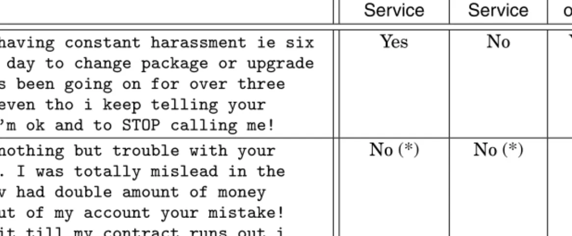
Training label cleaning has to do with the presence of mislabelled items in the train-ing data (see Figure 1 for two concrete examples). Of course, defintrain-ing what counts as a
Text Customer Network Tariff
Service Service or Value
I keep having constant harassment ie six calls a day to change package or upgrade this has been going on for over three months even tho i keep telling your staff i’m ok and to STOP calling me!
Yes No Yes (*)
Iv had nothing but trouble with your network. I was totally mislead in the shop. Iv had double amount of money taken out of my account your mistake! Cant wait till my contract runs out i wouldnt recommend you 2 anyone!
No (*) No (*) Yes
Fig. 1. Two (manually) mislabelled training documents. The 1st column lists the textual content of the documents, while the other columns indicate some among the classes that the human annotators were meant to assign. The context was a customer satisfaction survey by a telecommunications company to whom these authors provide text classification services; the goal of the classification is to spot reasons for dissatisfaction with the company. Labels marked with a “(*)” seem clear mislabellings on the part of the (junior) annotators who performed the annotation.
mislabelled example is itself tricky, because labelling a document is a subjective activ-ity. Different annotatorsa1anda2might in good faith disagree as to whether classcj
should be attributed or not to documentdi, a phenomenon calledintercoder disagree-ment. This problem is exacerbated when the meaning of the class is not clearcut: for instance, it is not always clear if a given product review should be classified asPositive
orNegative, or whether a given news article fits or not into classLifestyles.
For the purpose of this article we will simply assume that when annotator a2 at an organization inspects a set of labelled documents owned by the organization with the purpose of determining the quality of the labelling, and detects a label (originally attributed by annotatora1) she disagrees with, this counts as a mislabelled document. In other words, we are assuming that the judgment of the annotator who performs the quality check is more important that that of the annotator who had originally labelled the documents. There are several reasons for this assumption.
(1) In several organizations it is often the case that the original labelling is performed by annotators (usually called “coders”) as a part of their daily routine. In this rou-tine, throughput (i.e., number of annotated documents per unit of time) is an es-sential factor. As a result, the coders’ labelling activity may be error-prone.
Coders usually report to a more senior, superordinate “information specialist” who, in case labelled data are to be used for training an automated classifier (thereby generating a durable asset for the organization), may decide to double-check the labels originally attached by her coders. In this double-checking activity the re-sulting label quality is essential, while throughput is much less so. As a result, the judgments of the information specialist override those of the coders, and may be taken to be “the correct ones”.
(2) It is hardly the case that the coders are the originators of the classification scheme; as a result, they may have an imperfect understanding of the true meaning of the classes, which may further negatively affect the quality of the labels they attribute. On the contrary the information specialist, being more senior, may either be the originator of the classification scheme or may be its maintainer (i.e., the one that decides when and if it needs revision in order to better suit the changing needs
of the organization), which means that her understanding of the meaning of the classes is certainly higher than that of the coders. This is a further reason why the labels she decides to attribute are more reliable than those attributed by the coders.
(3) When coders perform the original labelling they tend to work in “routine mode”, sometimes with less-than-total commitment; an example is the (increasingly fre-quent) case in which annotation is performed via crowdsourcing (e.g., Mechanical Turk), yet another context in which fast turnaround (rather than label quality) is the main goal of the annotators [Grady and Lease 2010; Snow et al. 2008]. When an information specialist sets out to revise the labels attributed by her coders, she is instead likely to work in “double-checking mode”, which is obviously conducive to better labelling decisions.
(4) If the user interface coders work with displays up-front the titles of a list of doc-uments to be labelled, and only shows the body of a document if the annotator double-clicks on them, some coders will be happy to work from the titles alone, and this might be sufficient to correctly label most documents. However, for some documents the resulting labelling will be incorrect because the coders have not inspected the actual body of the document. This is another potential source of er-ror, and one the information specialist will not be prone to if, working in double-checking mode, she does indeed inspect the body of the document.
(5) If the actual task is multilabel classification (see Section 3 for details), coders might attribute one or two labels to a document and stop exploring the classifi-cation scheme for other potential classes that might apply, thus generating several false negatives. It is the experience of these authors that, when classifying texts for market research applications (see Esuli and Sebastiani [2010]), coders make a conscious effort to avoid false positives but a much smaller one to avoid false neg-atives. An information specialist double-checking the labelled documents would likely not incur in the same mistake.
For all these reasons we may confidently assume that, when a set of labelled data is double-checked with the purpose of correcting possible mislabellings and using it to train a classifier, the labels decided upon by the annotator who performs the re-vision are the “correct” ones. This assumption justifies the experimental protocol we will adopt in Section 5, and ultimately justifies the very endeavour of training label cleaning.
3. PRELIMINARIES
This work attempts to identify good TLC techniques for text classification (aka text categorization – TC), and for multilabel text classification (MLTC) in particular. Given a set of textual documents D and a predefined set of classes (aka categories)
C = {c1,. . .,cm}, MLTC can be defined as the task of estimating an unknown target
function: D×C → {−1,+1}, that describes how documents ought to be classified, by means of a functionˆ : D×C → {−1,+1}called theclassifier1; here,+1 and −1 represent membership and non-membership of the document in the class. Each docu-ment may thus belong to zero, one, or several classes at the same time. As usual, we accomplish MLTC by generatingmindependent binary classifiersˆj:D→ {−1,+1}, one for eachcj ∈ C, entrusted with the task of deciding whether a document belongs to class cj or not. Note that we here do not address the related problem of TLC for single-label, multiclass classification, where each document needs to be assigned one 1Consistently with most mathematical literature we use the caret symbol (ˆ) to indicate estimation.
and only one out ofm>2 candidate classes; we leave the investigation of this task to future work.
As the learner for generating our classifiers we use our in-house boosting-based learner, called MP-BOOST [Esuli et al. 2006]; classifiers obtained via boosting have consistently shown high accuracy in several learning tasks, while at the same time having strong justifications from computational learning theory [Schapire and Freund 2012]. MP-BOOSTis a variant of ADABOOST.MH [Schapire and Singer 2000] explic-itly optimized for multilabel settings, which has been shown in [Esuli et al. 2006] to obtain considerable effectiveness improvements with respect to ADABOOST.MH.
MP-BOOSTworks by iteratively generating, for each classcj, a sequenceˆ1j, . . . ,ˆSj of classifiers (calledweak hypotheses). A weak hypothesis is a functionˆsj : D → R, whereDis the set of documents andRis the set of the reals. The sign ofˆsj(di)(denoted bysgn(ˆsj(di))) represents the binary prediction ofˆsjon whetherdibelongs tocj, that is, sgn(ˆsj(di)) = +1 (resp., −1) means that di is predicted to belong (resp., not to belong) to cj. The absolute value of ˆsj(di) (denoted by | ˆsj(di)|) represents instead the confidence that ˆsj has in this prediction, with higher values indicating higher confidence.
At each iterationsMP-BOOSTtests the effectiveness of the most recently generated weak hypothesisˆsj on the training set and uses the results to update a distribution Dsjof weights on the training examples. The initial distributionD1jis uniform. At each iteration sall the weights Dsj(di)are updated, yielding Dsj+1(di), so that the weight assigned to an example correctly (resp., incorrectly) classified byˆsjis decreased (resp., increased). The weightDsj+1(di)is thus a measure of how ineffectiveˆ1j,. . .,ˆsjhave been in predicting whetherdi belongs tocjor not (denoted by j(di)). By using this distribution, MP-BOOSTgenerates a new weak hypothesisˆsj+1 that concentrates on the examples with the highest weights, that is, those that had proven harder to classify for the previous weak hypotheses.
The overall prediction on whether di belongs to cj is obtained as a sum ˆ j(d i) =
S
s=1ˆ j
s(di)of the predictions of the weak hypotheses. The final classifier ˆ jis thus acommittee ofSclassifiers, each classifier casting a weighted vote, with the vote be-ing the binary predictionsgn(ˆsj(di)) and the weight being the confidence| ˆsj(di)|of this prediction. For the final classifierˆ jtoo,sgn(ˆ j(di)) represents the binary pre-diction as to whetherdi belongs tocj, while| ˆj(di)|represents the confidence in this prediction.
See Esuli et al. [2006] for more details on these and other aspects of MP-BOOST. 4. THREE TECHNIQUES FOR TRAINING LABEL CLEANING
In the following, by aTLC techniqueρwe will mean a technique that, given a training setTrand a classcj, produces a rankingrρj(Tr)in which the elements ofTrare sorted in decreasing order of the likelihood that their manually assigned label forcjis wrong. Different techniques correspond to different ways of estimating this likelihood.
Note that, given a set of classesC= {c1,. . .,cm}, these techniques thus generatem different and independent rankings ofTr; no unified and/or merged ranking is gener-ated. This evokes an application scenario in which the user cleans the training data on a class-per-class basis, working on the classes for which the effectiveness is still low and disregarding the ones for which the effectiveness is already high enough, or
inspecting the different class-specific lists down to different depths depending on how much a given class needs improvement.
We now present three alternative TLC techniques. 4.1. The Confidence-Based Technique
For each cj ∈ C, the first technique (that we dub the confidence-based technique – CONF, in short) consists in
(1) training a classifierˆ jonTr;
(2) reclassifying thedi∈Trby means ofˆ j;
(3) ranking thedi∈Trin increasing order of theirˆj(d
i)·j(di)value. The product ˆj(d
i)·j(di) is the margin of an example as computed by the final classifier. Note that, whilej(di)is a value in{−1,+1},ˆ j(di)is a value in(−∞,+∞), soˆj(di)·j(di)is also in(−∞,+∞); a positive (resp., negative) value ofˆ j(di)·j(di) indicates a correct (resp., incorrect) binary prediction, while a high (resp., low) absolute value of The CONF technique thus corresponds to (a) top-ranking the examplesdi∈Tr thatˆ jhas misclassified, in decreasing order of the confidence| ˆj(d
i)|with whichˆ j has made its prediction, and (b) appending to this list the examplesdi∈Trthatˆ jhas correctly classified, in increasing order of the confidence| ˆj(di)|. Obviously, different rankings are produced for the differentcj∈C. The rationale of this technique is that, ifˆ jhas misclassified a training examplediwith high confidence, this means that the label forcjgiven todiby the human annotator is highly at odds with the labels forcj
that the human annotator has given to the other training examples, which indicates that the human annotator may well have mislabelleddiforcj.
4.2. The Nearest Neighbours Technique
For eachcj∈C, the second technique (that we dubthe nearest neighbours technique– NN) consists in ranking the training examples in terms of how inconsistent their label for cj is with the labels forcj of theirk nearest neighbours, for a predefined k. More formally, this technique consists in
(1) computing, for eachdi∈Tr, the value
ζ(di,cj)=
dz∈Trk(di)
sim(di,dz)·j(dz), (1) where sim(·,·) denotes a measure of similarity between documents and Trk(di) denotes thektraining examples most similar todi;
(2) ranking thedi∈Trin increasing order of theirζ(di,cj)·j(di)value.
For classcj, the examplesdiwith labels highly consistent with the labels of their neigh-bours will have highζ(di,cj)·j(di)values, which means that the ones with the lowest
ζ(di,cj)·j(d
i)values will be the ones with labels most dissimilar from those of their closest neighbours. Equation (1), of course, is that of the standard distance-weighted
k-NN learner (see e.g., [Yang 1994, 1999]), the only difference being that, while in the standard casej(d
z)ranges on {0,1}, in our case it ranges on{−1,+1}, which means that neighbours with a negative label forcjweigh negatively, instead of having no ef-fect, onζ(di,cj). This variant of thek-NN learner is discussed in Galavotti et al. [2000]. The NN technique is similar to the CONF technique, and it might be seen as an instantiation of CONF where the Galavotti et al. [2000] variant of thek-NN classifier is used as the learning method. One difference between NN and CONF is that in NN the
sign ofζ(di,cj)is, unlikeˆj(di)in CONF, not meant to represent the binary prediction of the classifier, since the decision threshold is not necessarily zero. A second, more significant difference is that in CONF the document di whose manually attributed label is being evaluated has also played the role of the training example in generating
ˆ
j, which is being used for the evaluation. This does not happen in the NN technique, sincediis not a member ofTrk(di).
4.3. The Committee-Based Technique
For each cj ∈ C, the third technique (that we dub the committee-based technique– COMM) consists in
(1) training a classifierˆjonTr; (2) reclassifyingTrby means ofˆ j;
(3) ranking thedi∈Trin increasing order of their
(ˆ j(d
i))·sgn(ˆ j(di))·j(di) value, where(ˆ j(d
i))is a nonnegative real number that measures theagreement among theSmembers ofˆ jon whetherdibelongs tocjor not.
This technique is based on the intuition that the examples most in need of inspection are the ones whichˆjhas misclassified (i.e., those such thatsgn(ˆj(di))·j(di)= −1) with the most widespread agreementamong itsSmembers. In other words, if the infor-mation that a training example provides to the training process is so inconsistent with that provided by the other training data as to have the members of the generated clas-sifier committee misclassify the example with widespread agreement, then it is likely that the example might be mislabelled. This technique will thus top-rank the training examples that the committee has misclassified and on which the S members of the committee agree most, mid-rank those on which there is disagreement, and bottom-rank those that the committee has classified correctly and on which theSmembers of the committee agree most.
The key difference between the first technique (CONF) and this technique is that here the confidence that a classifier committee has in a certain prediction is taken to coincide with the level of (weighted) agreement among its members, and not with the (weighted) sum of the individual opinions. As a measure of agreement among the S
members of the committee we have chosen to use 1σ, where σ denotesstandard devi-ation. This is a natural choice, given that the valuesˆ1j(di),. . .,ˆSj(di)are real num-bers: standard deviation thus enables the measurement of (dis)agreement by taking into account not only the polarity sgn(ˆsj(di)) of each member’s prediction, but also its confidence level| ˆsj(di)|, so that two members with views of different polarity are taken to disagree more if they are highly confident in their views, and less if they are not.2
4.4. The Distribution-Based Technique
Actually, there is a fourth technique (which we dubthe distribution-based technique– DIS) that might come to mind [Abney et al. 1999, Section 5]. For each cj ∈ C, this technique consists in (i) training the classifiersˆjonTr, and (ii) ranking thedi ∈ Tr in decreasing order of theDSj(di)value that MP-BOOSThas produced as a side effect of 2A previous version of this article [Esuli and Sebastiani 2009] contained a wrong, and ultimately unintuitive, version of this technique; the present article thus describes both a revised version of the technique and experiments run anew.
the learning process. The rationale of this technique is that, since the valueDSj(di)is a measure of how hard it has been, for the weak learners generated by the boosting iterations, to correctly reclassify di under cj, the training examples that maximize DSj(di) are the ones that have turned out the most difficult to make sense of during the boosting iterations. As a result, they are the ones whose label forcjis most highly at odds with the label forcjof the other training examples.3
The problem with the DIS technique is that it turns out to be equivalent to our first technique (CONF), in the sense that CONF and DIS always generate identical rankings, a fact that had never been noted in the literature.4
The only advantage that DIS provides over CONF is thus that there is no need to reclassify the training examples by means ofˆj, since the information needed for ranking is already available after training has occurred.
4.5. A Note about Generality
Before discussing the experiments it is worthwhile noting that, although we have de-scribed these techniques in the context provided by a boosting-based learner which generates confidence-rated predictions, all of these techniques can be used also in con-nection with other learners. More specifically, CONF only needs the classifier to re-turn a score of confidence in its own prediction, NN has no specific requirements, and COMM only require the classifier to consist of a committee of classifiers. Moreover, the discussed equivalence between CONF and DIS has the practical consequence of making available a technique equivalent to DIS to learners not based on boosting. 5. EXPERIMENTS
5.1. Experimental Protocol
In order to test our TLC techniques we use a standard MLTC dataset = Tr,Te
split into a training set Tr and a test set Te. We assume that Tr and Tecontain no mislabelled examples, and simulate the presence of mislabelled training examples by artificially “corrupting” a small numbert of training examples; we call = |Trt| the
corruption ratio. In what follows, “corrupting a training exampledifor classcj” means changing its label forcjfrom positive to negative (in this case we calldiafake negative for cj) or from negative to positive (a fake positive); byTr we denote the training set after corruption, and byFNjandFPjthe sets of fake negatives forcjand fake positives forcj, respectively. We use the term “fake” instead of “false” in order to avoid overload-ing the latter term. We will also use the term “genuine” as the opposite of “fake.”
We test two different corruption techniques, which we callrandom corruption(RC) and targeted corruption (TC). As the name implies, in RC the training examples to 3A similar technique would also be applicable when using SVMs as the learner, since SVMs assign, as a side-effect of training, a weightαito each training example that reflects how hard it has been for the generated classifier to reclassify it.
4We discovered this fact experimentally in the course of this work. A conversation with Robert Schapire, the inventor of boosting, later revealed that, while this phenomenon had never been observed before, ana posteriorijustification can be found in the theory that underlies the ADABOOST.MH algorithm, of which MP-BOOSTis a variant. Specifically, the reason is to be found in the fact that (as shown in the proof of Theorem 1 of [Schapire and Singer 1999])Dj
S+1(di)∝exp(−j(di)· ˆj(di)). Since CONF ranks thedi∈Tr in increasing order ofj(di)· ˆj(di)value, since DIS ranks them in decreasing order ofDj
S+1(di)value,
and since exp(x)is a monotonically increasing function of its argument, it follows that the two rankings are the same. This property applies not only to ADABOOST.MH but also, straightforwardly, to MP-BOOST(see [Esuli et al. 2006, Section 3]).
Table I. Percentagepfnof Corrupted Documents That Are Fake Negatives as a Function of the Corruption Ratio
REUTERS-21578 RCV1-V2 OHSUMED RC TC RC TC RC TC .001 0.7% 46.1% 2.8% 65.4% 0.2% 31.0% .010 0.9% 19.3% 3.1% 43.9% 0.1% 8.4% .050 0.8% 7.3% 3.1% 22.8% 0.1% 2.3% .100 0.8% 4.3% 3.1% 14.9% 0.1% 1.2%
corrupt are picked at random fromTr. For simplicity, the samettraining examples are corrupted for all classescj ∈ C. (This is absolutely equivalent to corrupting different training examples for the different classes, since our methods work on each of the classes independently.) TC is instead obtained by
(1) training the classifiersˆjonTr;
(2) reclassifying thedi∈Trby means of them;
(3) ranking, for eachcj∈C, the reclassified examples in increasing order of the confi-dence| ˆj(di)|thatˆjhad in classifying them;
(4) corrupting thettop-ranked ones.
The rationale of this technique is that the training examples thatˆ jclassifies with low confidence are more likely to be “borderline” examples for cj; as a result these examples, should they be manually labelled, would have a high likelihood of being mislabelled (either due to lack of experience or to lack of adequate time) by a human annotator. In other words, while RC simulates the corruption of a training set that might derive from, say, lack of commitment on the part of the human annotators (e.g., in crowdsourced annotation), TC simulates the corruption that might derive from in-complete or imperfect understanding of the semantics of the classes. While it is true that what counts as a borderline example to a human annotator might not count as borderline to a text classification system (and vice versa), targeted corruption makes at least a substantive step in the direction of identifying examples that are more likely to get mislabelled by annotators.
Unlike in RC, in TC we allow different training examples to be corrupted for different classescj∈C, since the same document might be controversial, or “borderline”, for one class but not for others.
Table I illustrates, for each of the datasets we use in this article (see Section 5.3 for a detailed description of them), for each corruption technique and for each corruption ratio, the percentagepfn =
m j=1|FNj|
m
j=1|FNj+FPj| ·100% of corrupted documents that are fake
negatives; obviously,pfp =100%−pfn. For random corruption this percentage tends to be fairly constant across the different corruption ratios (although different across datasets), which is obvious since it tends to coincide with the average class frequency of the entire dataset.
Table I also shows that, for a given corruption ratio,pfnis always higher (and usually much higher) for TC than for RC; for example, for REUTERS-21578 and=.001 the value ofpfnis 0.7% for RC and 46.1% for TC. The reason is that TC corrupts not random but “borderline” examples, and these proportionally include many more positives than random examples do.
The same table also shows that in targeted corruption, while fake positives tend to outnumber fake negatives, this tendency is increasingly marked as the corruption rate increases; for example, for REUTERS-21578 the value ofpfnis 46.1% for=.001 but only 4.3% for =.100. This is due to the fact that, as in most text classification
datasets, the number of genuinely positive examples is much smaller than the number of genuinely negative examples. As a result, as the number of documents to corrupt increases the number of positive documents that can be corrupted cannot increase proportionally.
5.2. Effectiveness Measures
In order to determine which among the three TLC techniques of Section 4 is the best we will measure how good each technique is at ranking thedi∈Trin such a way that the corrupted training examples are placed at the top of the ranking. To this end, it seems natural to adopt one of the measures routinely used for evaluating ad-hoc (ranked) retrieval. Of course, ad-hoc retrieval is all about ranking the “good” (i.e., relevant to the information need) examples higher than the bad ones, while TLC aims at ranking the “bad” (i.e., mislabelled) examples higher than the good ones; but this is obviously inessential.
As a measure of ranking quality we will choosemean average precision(MAP), which in our context is defined as follows. Let rρj(Tr) be the ranking for class cj realized according to TLC techniqueρ, of the corrupted training setTr, and let [rρj(Tr)]k be a binary predicate that returns 1 if the example at thek-th position inrρj(Tr)is corrupted for classcj, and 0 otherwise. We define theprecision at n of rρj(Tr)as
Pn(rρj(Tr))= 1 n n k=1 [rρj(Tr)]k. (2) We then define theaverage precision of rρj(Tr)as
AP(rρj(Tr))= |Tr| k=1Pk(r ρ j(Tr))·[r ρ j(Tr)]k |Tr| k=1[r ρ j(Tr)]k . (3)
Themean average precision(MAP) of TLC techniqueronTris finally defined as
MAP(r(Tr))= 1
|C|
cj∈C
AP(rρj(Tr)). (4)
Aside from a measure of TLC effectiveness we will also need a measure of MLTC effec-tiveness, so as to determine which effectiveness gains in classification can be obtained if TLC is performed. As a MLTC effectiveness measure that combines the contribu-tions ofprecision(π) andrecall(ρ) we have used the well-knownF1 function, defined as F1 = π2πρ+ρ = 2TP+2FPTP+FN, where TP, FP, and FN stand for the numbers of true positives, false positives, and false negatives, respectively. Note thatF1 is undefined when TP = FP = FN = 0; in this case we take F1 to equal 1, since the classifier has correctly classified all documents as negative examples. We compute both microav-eragedF1(denoted byFμ1) and macroaveragedF1(F1M).Fμ1 is obtained by (i) computing the category-specific valuesTPi,FPiandFNi, (ii) obtainingTPas the sum of theTPi’s (same for FP and FN), and then (iii) applying the F1 = 2TP+2FPTP+FN formula. F1M is obtained by first computing the category-specific F1 values and then averaging them across thecj’s.
Section 5.4 reports the results of our experiments with the three TLC techniques of Section 4, each tested under two different corruption techniques, four different corrup-tion ratios, and three different datasets.
5.3. The Datasets
In our experiments we have used the REUTERS-21578, RCV1-V2, and OHSUMED datasets.
REUTERS-21578 is probably still the most widely used benchmark in MLTC re-search.5 It consists of a set of 12,902 news stories, partitioned (according to the “ModApt´e” split we have adopted) into a training set of 9,603 documents and a test set of 3,299 documents. The documents are labelled by 118 categories; in our experi-ments we have restricted our attention to the 115 categories with at least one positive training example. The average number of categories per training document is 1.005, the number of positive training examples per category ranges from a minimum of 1 to a maximum of 2877, and the average balance ratio6in the training set isB=.017.
REUTERSCORPUSVOLUME1 version 2 (RCV1-V2)7is a more recent MLTC bench-mark made available by Reuters and consisting of 804,414 news stories produced by Reuters from 20 Aug 1996 to 19 Aug 1997. In our experiments we have used the “LYRL2004” split, defined in Lewis et al. [2004], in which the (chronologically) first 23,149 documents are used for training and the other 781,265 are used for testing. Of the 103 “Topic” categories, in our experiments we have restricted our attention to the 101 categories with at least one positive training example. Consistently with the evaluation presented in [Lewis et al. 2004], (i) also categories placed at internal nodes in the hierarchy are considered in the evaluation, and (ii) as positive training exam-ples of these categories we use the union of the positive examexam-ples of their subordinate nodes, plus their “own” positive examples. The average number of categories per train-ing document is thus 3.184, the number of positive traintrain-ing examples per category ranges from a minimum of 2 to a maximum of 10786, and the average balance ratio in the training set isB=.063.
The OHSUMED test collection [Hersh et al. 1994] consists of a set of 348,566 MED-LINE references spanning the years from 1987 to 1991. Each entry consists of sum-mary information relative to a paper published on one of 270 medical journals. The available fields are title, abstract, MeSH indexing terms, author, source, and publica-tion type. Not all the entries contain abstract and MeSH indexing terms. In our experi-ments we have scrupulously followed the experimental setup presented in Lewis et al. [1996]. In particular, (i) we have used for our experiments only the 233,445 entries with both abstract and MeSH indexing terms; we have used the entries relative to years 1987 to 1990 (183,229 documents) as the training set and those relative to year 1991 (50,216 documents) as the test set; (iii) as the categories on which to perform our experiments we have used the “main heading” part of the MeSH index terms assigned to the entries.8Concerning this latter point, we have restricted our experiments to the
5http://www.daviddlewis.com/resources/testcollections/∼reuters21578/ 6We define theaverage balance ratioin the training set as the value
B=(1− 1 |C| ci∈C ||Tr+i | − |Tr−i | |Tr| |), where|Tr+
i |(resp., |Tr−i |) is the number of positive (resp., negative) training examples for classci. The
average balance ratio isB=1 only if all classes are perfectly balanced (i.e., they have an equal number of positive and negative training examples) and is 0 if all classes are perfectly imbalanced (i.e., each of them has either no positive training examples or – uncharacteristically – no negative training examples). 7http://trec.nist.gov/data/reuters/reuters.html
8MeSH index terms consist of a main heading optionally qualified with subheadings and/or importance markers. For example, in the MeSH index termOxytocin/*AA/GE, the main heading isOxytocin. Several MeSH index terms may be assigned to the same entry, which means this is a multilabel TC task.
97 MeSH index terms that belong to theHeart Disease(HD) subtree of the MeSH tree, and that have at least one positive training example. This is the only point in which we deviate from Lewis et al. [1996], which experiments only on the 77 most frequent MeSH index terms of the HD subtree. The average number of categories per training document is 0.130 (many training documents are unlabelled, and just serve as nega-tive training examples for all classes), the number of posinega-tive training examples per category ranges from a minimum of 1 to a maximum of 4075, and the average balance ratio in the training set isB=.003.
There are three main reasons why we have chosen exactly these datasets:
(1) All these datasets are publicly available and very widely used in text classifica-tion research, which allows other researchers to easily replicate the results of our experiments.
(2) RCV1-V2 and OHSUMED are among the largest datasets used to date in text classification research, which lends robustness to our results.
(3) For at least two (REUTERS-21578 and RCV1-V2) of our chosen datasets, the as-sumption that the uncorrupted training sets do not contain mislabelled training examples (see Section 5.1) is probably more justified than for any other text clas-sification datasets available in research, since the document labelling of these datasets has undergone a lot of quality checking from Reuters editors and text classification researchers alike [Lewis 2004; Lewis et al. 2004].
In all the experiments discussed in this article stop words have been removed, punc-tuation has been removed, all letters have been converted to lowercase, numbers have been removed, and stemming has been performed by means of Porter’s stemmer. Word stems are thus our indexing units. Since MP-BOOSTrequires binary input, only their presence/ absence in the document is recorded, and no weighting is performed as far as MP-BOOST is concerned. Documents are instead weighted (by standard cosine-normalized tfidf) (i) for the sake of computing the interdocument similarity values required by theNNtechnique of Section 4.2, and (ii) for the further experiments with the SVM learner that we will later describe in Section 6.
5.4. Results and Discussion
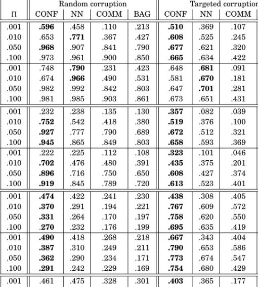
5.4.1. Evaluating the Quality of Training Label Cleaning.Table II reports MAP values ob-tained by ranking the corrupted training sets by means of the three TLC techniques (CONF, NN, COMM); the meaning of the fourth column (labelled BAG) will be made clear in Section 6.2. For each tested corpus, (a) we report results for the full set of classes, and (b) from these results we single out those concerning the 30 most infrequent classes and report them separately. (The meaning of the rows labelled “OHSUMED-S” will be clarified in Section 5.4.2.) The reason we pay special atten-tion to the mostinfrequentclasses (unlike many researchers who often report results only for the most frequent classes of a collection) is that they are usually the classes for which standard supervised learning techniques produce the lowest classification effectiveness. This means that they are the classes most in need of effectiveness im-provements, by TLC or other techniques: a user might typically engage in TLC for these highly problematic classes, and disregard the classes for which high enough ac-curacy has already been achieved.
In all the experiments MP-BOOSThas been run with a numberSof iterations fixed to 1,000. For the NN technique, as the sim(·,·) measure of inter-document similar-ity we have used the inner product of the cosine-normalizedtfidf vectors of the two documents. For the same technique we have used the value k = 45, since in using
Table II.
Mean average precision (MAP) of the four TLC techniques (CONF, NN, COMM, BAG) on the full set of classes (top 4 rows) and on the 30 most infrequent classes (bottom 4 rows) of REUTERS-21578, RCV1-V2, OHSUMED, and OHSUMED-S.Boldface indi-cates a statistically significant (two-tailed paired t-test on average precision value over categories,P<0.01) best performer for a given combination of corruption ratio (), cor-ruption method, and dataset.
Random corruption Targeted corruption
CONF NN COMM BAG CONF NN COMM BAG
R EUTERS -21578 FULL S ET .001 .596 .458 .110 .213 .510 .369 .107 .230 .010 .653 .771 .367 .427 .608 .525 .245 .291 .050 .968 .907 .841 .790 .677 .621 .320 .340 .100 .973 .961 .900 .850 .665 .634 .422 .457 30 I NFR .001 .748 .790 .231 .423 .648 .681 .091 .235 .010 .674 .966 .490 .531 .581 .670 .181 .287 .050 .982 .992 .842 .803 .647 .701 .281 .361 .100 .981 .985 .903 .861 .673 .651 .431 .439 RCV1-V 2 F ULL S ET .001 .232 .238 .135 .130 .357 .082 .039 .278 .010 .752 .542 .418 .380 .519 .376 .100 .384 .050 .927 .777 .790 .689 .672 .512 .321 .430 .100 .945 .865 .849 .803 .658 .593 .369 .461 30 I NFR .001 .222 .225 .112 .108 .323 .101 .046 .181 .010 .702 .476 .480 .391 .435 .375 .201 .297 .050 .896 .716 .750 .650 .608 .427 .374 .381 .100 .919 .845 .789 .720 .613 .523 .401 .413 OHSUMED F ULL S ET .001 .474 .422 .241 .230 .438 .308 .405 .392 .010 .370 .291 .194 .221 .767 .609 .572 .432 .050 .331 .264 .170 .197 .758 .620 .550 .467 .100 .270 .232 .176 .199 .695 .635 .419 .403 30 I NFR .001 .490 .418 .268 .218 .667 .343 .404 .383 .010 .387 .310 .249 .211 .790 .653 .586 .443 .050 .362 .290 .234 .171 .773 .674 .547 .466 .100 .291 .242 .229 .169 .754 .680 .429 .411 OHSUMED-S F ULL S ET .001 .461 .475 .328 .301 .403 .365 .177 .104 .010 .667 .688 .566 .610 .576 .549 .413 .401 .050 .917 .870 .856 .803 .651 .642 .521 .507 .100 .948 .898 .893 .841 .669 .650 .527 .509 30 I NFR .001 .544 .555 .419 .423 .564 .526 .224 .209 .010 .832 .854 .738 .740 .631 .643 .351 .339 .050 .953 .915 .883 .831 .671 .669 .485 .458 .100 .969 .933 .921 .873 .693 .683 .526 .513
k-NN as a learner for TC Yang [1999], using REUTERS-21578, has found this value to yield the best effectiveness (and has found negligible differences among values of
k∈[30, 65]).9
9In operational conditions, if one had to pick the optimal value ofkfor the NN technique, one might well classify all the training documents via thek-NN classifier (using each training document as test and the other training documents as training), compute the resulting classification accuracy, do all this for various values ofk, pick the value ofkthat has given the best classification accuracy, and use this value ofkfor per-forming the cleaning, on the assumption that what works best for classification also works best for training data cleaning. This means that, despite appearances to the contrary, the given protocol of choosing a value ofkthat has proven optimal in classification experiments on the very same dataset we use is legitimate.
A “trivial” baseline to the results of Table II is the expected MAP value of therandom ranker (RR), that is, the algorithm which generates random document rankings. As proven in Resta [2012], the expected AP value of the RR is equal to
AP(RR())= tj−1 n−1+
(n−tj)Hn
n(n−1) . (5)
In our setting,tjcorresponds to the number of documents which are mislabelled forcj andnto the number of documents that need to be ranked (i.e.,n = |Tr|);Hndenotes then-th harmonic number (i.e.,Hn =nk=11k). In the hypothesis (which is indeed al-ways assumed true in our experiments) that the numbertjof mislabelled documents is the same for all classescj∈C, this is obviously also the expectedmeanAP value of the RR. Actual computation of this formula shows that MAP(RR())is approximated by
t
n (and in an especially accurate way for large values ofn), which in our case coincides with the corruption ratio. Since for all of our datasets and corruption ratios approx-imating Equation (5) to the third decimal digit exactly yields , the first column of Table II alsode facto indicates the trivial baseline for the experiments in the corre-sponding row.
There are several insights that can be gained from observing the results of Table II. The first observation is that, since picking training examples at random is the only method one can adopt when wanting to perform TLC, unless equipped with a specific TLC technique such as CONF, NN or COMM, the improvement that the three TLC techniques display in Table II over the baseline of Column 1 is considerable.
A second observation is that, with few exceptions and all other things being equal, each technique performs better for random corruption than for targeted corruption. This is intuitive, since mislabelled training examples inserted at random in the train-ing set tend to be easier to spot, since their labels tend to be more blatantly wrong; conversely, targeted corruption alters the label of examples which are borderline any-way, and their altered label is thus much more difficult to recognize as such for any
technique. By averaging all the figures contained in Table II we obtain a MAP value of .554 for random corruption and a value of .487 for targeted corruption.10 (We will informally call the values resulting from such averages the “TII-average MAP values.”) The third observation is that, among the three competing TLC techniques, CONF is a clear winner and COMM is a clear loser. In the vast majority of testing situations, CONF is either superior (in a statistically significant sense, two-tailed paired t-test on average precision value over categories,P <0.01) to both other techniques, or is not inferior (also in a statistically significant sense) to any of them. The COMM technique obtains instead, in almost all situations, results inferior (and often radically so) to CONF and NN. The TII-average MAP values are .625 for CONF, .549 for NN, and .388 for COMM. The CONF technique tends to be the better one on the RCV1-V2 and OHSUMED datasets, while the situation is less clearcut on REUTERS-21578. All in all, both techniques turn out to be respectable contenders, often achieving (sometimes surprisingly) high MAP values in absolute terms. We conjecture that the reason for the bad performance of COMM may be found in the fact that MP-BOOSTgenerates a committee of classifiers that arenotindependent of each other. Indeed, each member
ˆ
j
sof the committee strongly depends on the previously generated memberˆsj−1, since the former is generated according to the distribution resulting from applying ˆsj−1 to Tr. As a consequence, agreement is probably not something one could reasonably 10In the computation of these averages, and of other similar ones that will be discussed in the rest of this article, we disregard the values from the rows marked OHSUMED-S since, as will be apparent from Section 5.4.2, they would duplicate values from the rows marked OHSUMED and would thus bias the final results.
expect from the members of this kind of committee, since sharp disagreement may derive from reasons different from a bad label, such as the different emphasis that the different members place, by construction, on a given training example.
A fourth insight we can gain by looking at Table II is that MAP tends to increase with the corruption ratio, and may reach extremely high values for high values of
. The TII-average MAP values are 0.294 for = .001 (i.e., 0.1% of the documents are corrupted), 0.427 for =.010, 0.534 for=.050, and 0.552 for=.100. These high values of MAP are not a trivial result since, although higher corruption ratio means that there are many mislabelled examples, this does not make them easier to spot: possibly quite the contrary, since the ratio between correctly labelled and mis-labelled documents decreases, which means that the mismis-labelled documents are less inconsistent with the rest. High MAP values for high corruption ratio is very good news, since this means that if we have reasons to believe that our training set is ex-tremely low-quality, we know that our time in cleaning it will not be wasted, since these techniques will place many of the bad examples near the top of the ranking.11 Note that, when the corruption ratio is high and the class is infrequent, the number of corrupted documents may well exceed the number of positive instances of the class. (For instance, the 30 most infrequent classes of REUTERS-21578 have at most 2 pos-itive training examples each (out of the total 9,603 training examples), which means that this problem occurs even for a modest corruption ratio such as = .001.) As a result, in the corrupted training set the number of fake positives may well exceed the number of genuine positives. In this case, the good MAP results are due to the discrim-inating power of the (genuine) negative examples; for instance, the NN technique spots many fake positives since each of them lies, in the space of examples, close to many negative examples, which means that itsζ score (see Equation (1)) is extremely low. Similar arguments apply to the CONF and COMM techniques. We can also observe that there is no radical or systematic difference between the way our techniques work on the full set of classes and the way they work on the 30 most infrequent classes. While substantial differences are observed for some specific combinations (e.g., CONF on REUTERS-21578 corrupted via random corruption with = .001), these differ-ences are not systematic. To witness, the TII-average MAP values are .441 for the full set and .463 for the 30 most infrequent classes.
5.4.2. Strange News from Planet OHSUMED.As can be noticed by looking at Table II, when perturbed via random corruption the OHSUMED collection displays a quali-tatively different behaviour from the other two collections; in fact, while MAP tends to increase with in all other cases (i.e., when targeted corruption is used, or when the other two collections are involved), it tends to decrease when random corruption is applied to OHSUMED.
We conjecture that this strange phenomenon might be due to the fact that OHSUMED exhibits a much smaller average balance ratio (B=.003) than the other two collections (B=.017 for REUTERS-21578,B=.063 for RCV1-V2). This depends on the fact that its training set contains a huge amount of documents (more than 93% of the entire training set) that do not belong to any class, and that originally belonged to other subtrees of the MeSH tree.
In order to test this conjecture we have run additional experiments on a collection (that we here call OHSUMED-S) obtained from OHSUMED by retaining only the 11Note that a higher corruption ratio means highera prioriprobability that MAP is high, as witnessed by the fact that the expected MAP of the random ranker grows linearly with the corruption ratio. But this factor alone does not justify the very high MAP values we reach for high corruption ratios, as shown by the fact that the MAP of our techniques grows with the corruption ratio much faster than the expected MAP of the random ranker.
documents with at least one label in the HD subtree. The OHSUMED-S training set thus contains 12,358 documents, and its average balance ratio in the training set is
B=.020, much higher than the one of the full OHSUMED (B=.003) and similar to the one of the REUTERS-21578 collection (B=.017).
The results of these additional experiments, displayed in the last eight rows of Table II, essentially confirm our hypothesis, since they are qualitatively similar to those observed for REUTERS-21578 and RCV1-V2, and sharply different from those for the entire OHSUMED. The same similarity among REUTERS-21578, RCV1-V2, and OHSUMED-S (and their dissimilarity from OHSUMED) will be observed from Tables III and IV, to be discussed in the following sections
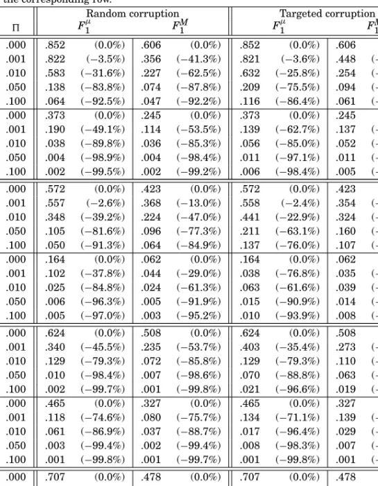
5.4.3. Evaluating the Effects of Noise. Table III reports instead the micro- and macro-averaged F1 values obtained by the classifiers generated via MP-BOOST before and after corruption, that is, after training either on the uncorrupted or on the corrupted training sets. This is an indication of the improvement in classification effectiveness one might obtain byfullycleaning the original training set when it contains noise at the corruption ratios indicated. Results are reported for the full set of classes and for the 30 most infrequent classes of our two datasets.
One insight that this table enables is that random corruption is usually more dam-aging to effectiveness than targeted corruption, and this fact tends to become evident as the corruption rate increases. That targeted corruption may have less disruptive ef-fects can be explained by the fact that TC introduces mislabellings on documents that are likely borderline examples anyway, that is, documents that two human annotators might legitimately label in different ways. Mislabelling them may hurt classification accuracy in the thin region of document space close to the surface that separates the positives from the negatives, but is not likely to affect accuracy elsewhere. Conversely, random corruption may have effects anywhere in document space, and may seriously mislead the classifiers even on cases that would be clearcut otherwise.
A second fact that immediately jumps to the eye is that the decrease in effectiveness deriving from corruption is considerable even for very modest corruption rates (e.g.,
=.001, i.e., 0.1%), and already becomes disastrous for slightly less modest ones (e.g.,
=.010). For instance, for a = .001 targeted corruption rate (which corresponds to roughly 10 mislabelled training documents in a training set of more than 9,600 documents), removing the mislabellings from the REUTERS-21578 training set makes
F1μjump from .821 to .852 for the full set of classes. This is a 3% relative improvement, that in the ’90s has taken years of improvement in TC technology to achieve. This shows that one mislabelled document in a thousand can single-handedly defy the efforts of many TC researchers at improving effectiveness.
While the percentages of deterioration are high throughout the table, there seems to be a correlation between deterioration and average balance ratio of the training set. In fact, recall from Section 5.3 that this ratio isB = .003 for OHSUMED,B= .017 for REUTERS-21578, andB=.063 for RCV1-V2. The three datasets are in the same order when it comes to deterioration; for example, the deterioration inFM1 at=.001 (full set of classes, targeted corruption) is −46.3% for OHSUMED, −26.1% for REUTERS-21578, and−16.3% for RCV1-V2. The fact that, for all three datasets, the deterioration radically increases when we move to the set of the 30 most infrequent categories, reinforces the point. This may be explained by the fact that learning a clas-sifier in the presence of strong imbalance (i.e., few positive training examples) is hard, and even a moderate corruption ratio can be disruptive on the effectiveness of the clas-sifier when the positive training examples are, relatively to the entire training set, few. The third insight that Table III suggests is that the deterioration in effectiveness resulting from corruption is larger for the more infrequent classes. For instance, in
Table III.
Micro- and macro-averagedF1 values of the classifiers generated by MP-BOOST for the full set of classes (5 top rows) and for the 30 most infrequent classes (5 bottom rows) of
REUTERS-21578, RCV1-V2, OHSUMED, and OHSUMED-S after corruption, as a
func-tion of the corrupfunc-tion ratio. Percentages indicate the relative deterioration in effective-ness with respect to the uncorrupted training set, which corresponds to the=.000 (no corruption) rows. The values in the third column are also a (trivial) baseline for the experi-ments in the corresponding row.
Random corruption Targeted corruption
Fμ1 FM1 Fμ1 F1M R EUTERS -21578 F ULL S ET .000 .852 (0.0%) .606 (0.0%) .852 (0.0%) .606 (0.0%) .001 .822 (−3.5%) .356 (−41.3%) .821 (−3.6%) .448 (−26.1%) .010 .583 (−31.6%) .227 (−62.5%) .632 (−25.8%) .254 (−58.1%) .050 .138 (−83.8%) .074 (−87.8%) .209 (−75.5%) .094 (−84.5%) .100 .064 (−92.5%) .047 (−92.2%) .116 (−86.4%) .061 (−89.9%) 30 I NFR .000 .373 (0.0%) .245 (0.0%) .373 (0.0%) .245 (0.0%) .001 .190 (−49.1%) .114 (−53.5%) .139 (−62.7%) .137 (−44.1%) .010 .038 (−89.8%) .036 (−85.3%) .056 (−85.0%) .052 (−78.8%) .050 .004 (−98.9%) .004 (−98.4%) .011 (−97.1%) .011 (−95.5%) .100 .002 (−99.5%) .002 (−99.2%) .006 (−98.4%) .005 (−98.0%) RCV1-V 2 FULL S ET .000 .572 (0.0%) .423 (0.0%) .572 (0.0%) .423 (0.0%) .001 .557 (−2.6%) .368 (−13.0%) .558 (−2.4%) .354 (−16.3%) .010 .348 (−39.2%) .224 (−47.0%) .441 (−22.9%) .324 (−23.4%) .050 .105 (−81.6%) .096 (−77.3%) .211 (−63.1%) .160 (−62.2%) .100 .050 (−91.3%) .064 (−84.9%) .137 (−76.0%) .107 (−74.7%) 30 I NFR .000 .164 (0.0%) .062 (0.0%) .164 (0.0%) .062 (0.0%) .001 .102 (−37.8%) .044 (−29.0%) .038 (−76.8%) .035 (−43.5%) .010 .025 (−84.8%) .024 (−61.3%) .063 (−61.6%) .039 (−37.1%) .050 .006 (−96.3%) .005 (−91.9%) .015 (−90.9%) .014 (−77.4%) .100 .005 (−97.0%) .003 (−95.2%) .010 (−93.9%) .008 (−87.1%) OHSUMED F ULL S ET .000 .624 (0.0%) .508 (0.0%) .624 (0.0%) .508 (0.0%) .001 .340 (−45.5%) .235 (−53.7%) .403 (−35.4%) .273 (−46.3%) .010 .129 (−79.3%) .072 (−85.8%) .129 (−79.3%) .110 (−78.3%) .050 .010 (−98.4%) .007 (−98.6%) .070 (−88.8%) .063 (−87.6%) .100 .002 (−99.7%) .001 (−99.8%) .021 (−96.6%) .019 (−96.3%) 30 I NFR .000 .465 (0.0%) .327 (0.0%) .465 (0.0%) .327 (0.0%) .001 .118 (−74.6%) .080 (−75.7%) .134 (−71.1%) .139 (−57.6%) .010 .061 (−86.9%) .037 (−88.7%) .017 (−96.4%) .029 (−91.0%) .050 .003 (−99.4%) .002 (−99.4%) .008 (−98.3%) .007 (−97.9%) .100 .001 (−99.8%) .001 (−99.7%) .001 (−99.8%) .001 (−99.7%) OHSUMED-S F ULL S ET .000 .707 (0.0%) .478 (0.0%) .707 (0.0%) .478 (0.0%) .001 .539 −(23.8%) .422 −(11.6%) .526 −(25.6%) .396 −(17.1%) .010 .459 −(35.1%) .279 −(41.7%) .431 −(39.0%) .257 −(46.3%) .050 .215 −(69.6%) .141 −(70.6%) .171 −(75.8%) .147 −(69.3%) .100 .177 −(75.0%) .119 −(75.2%) .093 −(86.8%) .095 −(80.1%) 30 I NFR .000 .320 (0.0%) .314 (0.0%) .320 (0.0%) .314 (0.0%) .001 .093 −(70.9%) .284 −(9.6%) .107 −(66.6%) .294 −(6.5%) .010 .022 −(93.2%) .045 −(85.6%) .032 −(90.0%) .071 −(77.5%) .050 .008 −(97.4%) .008 −(97.4%) .015 −(95.4%) .013 −(95.8%) .100 .002 −(99.4%) .002 −(99.3%) .006 −(98.2%) .005 −(98.3%)
the REUTERS-21578 case discussed earlier ( =.001), while the deterioration inFμ1
brought about by targeted corruption for the full set of classes is from .852 to .821 (−3.7%), for the 30 most infrequent classes the deterioration is from .373 to .139 (−62.8%)! The same effect may be observed by looking at theFM
1 results (instead of
F1μ) across the entire table: the improvements resulting from performing TLC are much larger forF1Mthan forF1μ, due to the fact thatF1μis not much influenced by the results on the infrequent classes, while FM1 is. It is not hard to see why the effect of even a few mislabelled training examples on the classification accuracy for infrequent classes can be so large. Given a class with very few positive training examples, mislabelling even one or a handful negatives as positives can severely alter the set of positive training examples, while mislabelling even one or a handful of positives as negatives has the double effect of depleting the already slim set of positive examples and confusing the learner, by presenting it with negative training documents that are very similar to the remaining positive ones. It is also likely that, given a class with few positive training examples, the presence of corrupted training examples close to the separating surface generates so much uncertainty in the classifier that it may often decide to vote negative so as to maximize accuracy. This may often be detrimental to
F1, since zero recall meansF1 =0.
Similar observations also hold for random corruption and for the other two datasets. For reasons of space we do not separately report the results on the (|C| −30) most frequent classes of our two datasets. In a nutshell, on these classes the decrease inFμ1
is very similar to the decrease on the full set of classes (sinceFμ1 is mostly influenced by the behaviour on the most frequent classes), while the decrease in F1M is smaller than the decrease in the full set of classes (since FM1 is equally influenced by all the classes inC).
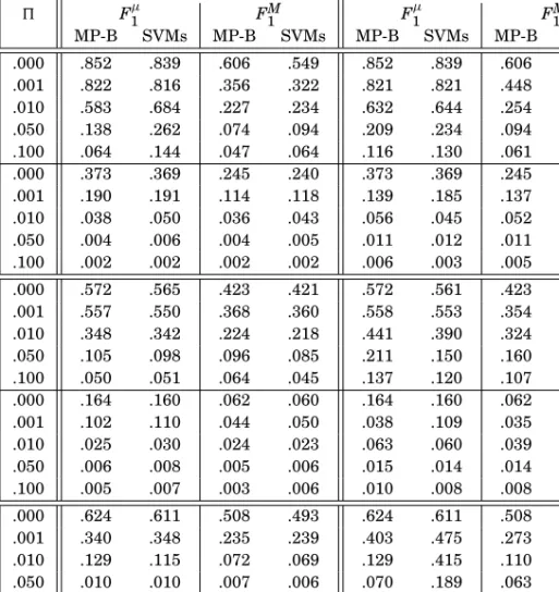
5.4.4. Evaluating the Effects of Cleaning. Note that Table III only gives us a picture of the improvement that might be obtained by cleaning the entire training set. Aside from probably being too expensive in many real-world situations, this is something that would defy the purpose of the TLC techniques we have presented. A study should thus be performed that, for any combination of TLC technique, corruption method, corruption ratio, and dataset, plots the effectiveness of the classifiers generated after TLC has been performed, as a function ofK, the number of top-ranked training exam-ples that the human annotator has inspected for misclassifications. This is obviously a daunting experimentation, since for each such combination and each value ofK the classifiers should be retrained from scratch and the test examples should be relabelled anew. More modestly, in Table IV we provide a sample such experiment, in which for the two different corruption methods, four corruption ratios, and all our three datasets, we test the effectiveness values resulting from
(1) ranking the training documents via the CONF technique;
(2) “uncorrupting” the corrupted documents found at the topK = |100Tr| positions (i.e., 1% of the total) in the ranking;
(3) training the classifiers on this partially cleaned training set; (4) classifying the test set via the classifiers thus generated.
For instance, on REUTERS-21578 with targeted corruption and = .001, the MAP value of .510 that CONF obtains (see Table II) guarantees thatFμ1, which corruption had reduced from .852 to .821, jumps back to .850, and that FM1 , which corruption had reduced from .606 to .448, jumps back to .498. What we may also observe from Table IV is that, unsurprisingly, high values of PK (precision at K) lead to higher