FULL LENGTH ARTICLE
Comparison of GIS-based interpolation methods
for spatial distribution of soil organic carbon (SOC)
Gouri Sankar Bhunia
a, Pravat Kumar Shit
b,*, Ramkrishna Maiti
ca
Bihar Remote Sensing Application Center, IGSC-Planetarium, Adalatganj, Bailey Road, Patna 800001, Bihar, India
bDept. of Geography, Raja N.L. Khan Women’s College, Gope Palace, Medinipur 721102, West Bengal, India c
Dept. of Geography and Environment Management, Vidyasagar University, Medinipur 721102, West Bengal, India
Received 17 October 2015; revised 31 January 2016; accepted 7 February 2016
KEYWORDS
Soil organic carbon; Deterministic interpolation; Geostatistical interpolation; Spatial variation;
GIS
Abstract The ecological, economical, and agricultural benefits of accurate interpolation of spatial distribution patterns of soil organic carbon (SOC) are well recognized. In the present study, differ-ent interpolation techniques in a geographical information system (GIS) environmdiffer-ent are analyzed and compared for estimating the spatial variation of SOC at three different soil depths (0–20 cm, 20–40 cm and 40–100 cm) in Medinipur Block, West Bengal, India. Stratified random samples of total 98 soils were collected from different landuse sites including agriculture, scrubland, forest, grassland, and fallow land of the study area. A portable global positioning system (GPS) was used to collect coordinates of each sample site. Five interpolation methods such as inverse distance weighting (IDW), local polynomial interpolation (LPI), radial basis function (RBF), ordinary krig-ing (OK) and Empirical Bayes krigkrig-ing (EBK) are used to generate spatial distribution of SOC. SOC is concentrated in forest land and less SOC is observed in bare land. The cross validation is applied to evaluate the accuracy of interpolation methods through coefficient of determination (R2) and
root mean square error (RMSE). The results indicate that OK is superior method with the least RMSE and highestR2value for interpolation of SOC spatial distribution.
Ó2016 The Authors. Production and hosting by Elsevier B.V. on behalf of King Saud University. This is an open access article under the CC BY-NC-ND license (http://creativecommons.org/licenses/by-nc-nd/4.0/).
1. Introduction
Spatial variability of soil organic carbon (SOC) is an impor-tant indicator of soil quality, as well as carbon pools in the ter-restrial ecosystem and it is important in ecological modeling,
environmental prediction, precision agriculture, and natural resources management (Wei et al., 2008; Zhang et al., 2012; Liu et al., 2014). Revealing the characteristics of SOC’s spatial pattern will provide the basis for evaluating soil fertility, and assist in the development of sound environmental management policies for agriculture. Scientific management of SOC nutrient is important for its sustainable development in agricultural sys-tem. So, there is a need of adequate information about spatio-temporal behavior of SOC over a region. SOC measurements, however, are inherently expensive and time consuming, particularly during the installation phase, which requires soil sampling. Consequently, the number of soil sampling that is
* Corresponding author.
Peer review under responsibility of King Saud University.
Production and hosting by Elsevier
Journal of the Saudi Society of Agricultural Sciences (2016)xxx, xxx–xxx
King Saud University
Journal of the Saudi Society of Agricultural Sciences
www.ksu.edu.sa
www.sciencedirect.com
available in a given area is often relatively sparse and does not reflect the actual level of variation that may be present. There-fore, accurate interpolation of SOC at unsampled locations is needed for better planning and management.
Different statistical and geostatistical approaches have been used in the past to estimate the spatial distribution of SOC (Kumar et al., 2012, 2013). Classical statistics could not make out the spatial allocation of soil properties at the unsampled locations. Geostatistics is an efficient method for the study of spatial allocation of soil characteristics and their inconsis-tency and reducing the variance of assessment error and execu-tion costs (Saito et al., 2005; Liu et al., 2014; Behera and Shukla, 2015). Earlier researchers have applied geospatial tech-niques to appraise spatial association in soils and to evaluate the geographical changeability of soil characteristics (Wei et al., 2008).Zare-mehrjardi et al. (2010), reported that ordi-nary kriging (OK) and cokriging methods were better than inverse distance weighting (IDW) method for prediction of the spatial distribution of soil properties. Robinson and Metternicht (2006) used three different techniques including kriging, IDW and Radial basis function (RBF) for prediction of the levels of the soil salinity, acidity and organic matter.
Pang et al. (2011)reported that ordinary kriging is most com-mon type of kriging in practice and provides an estimate of surface maps of soil properties.
Hussain et al. (2014)reported that Empirical Bayes kriging (EBK) is most suitable for spatial prediction of total dissolved solids (TSD) in drinking water.Mirzaei and Sakizadeh (2015)
reported that EBK model is best of all the geostatistical models such as OK and IDW for estimation of groundwater contamination.
These five widely used interpolation methods (RBF, IDW, OK, LPI and EBK models) have led to the quest about which is most appropriate in prediction of soil organic carbon in deferent soil depth. Therefore, the objective of this study was to conduct a thorough comparison of the GIS based interpolation techniques for estimating the spatial distribution of SOC in Medinipur Block, West Bengal, India, and apply cross validation to evaluate the accuracy of interpolation
method through the root mean square error (RMSE) measurement.
2. Materials and methods 2.1. Study area
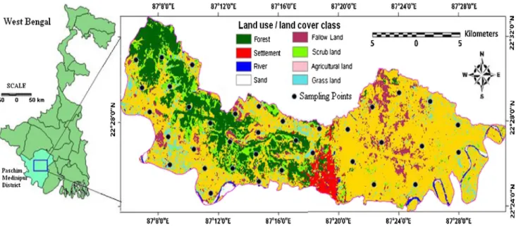
The study was conducted in Medinipur block of Paschim Med-inipur district in West Bengal (India). It is extended between 22°2304500N–22°3205000N latitude and 87°0504000E–87°3100100E longitude covering an area of 353 sq km (Fig. 1). The area is dry and the land surface of the block is characterized by red lateritic covered area, flat alluvial and deltaic plains. Extremely rugged topography is seen in the western part of the block and rolling topography is experienced in lateritic covered area (Shit et al., 2013). The maximum temperature recorded in April is 43°C and minimum temperature is 9°C. The average annual rainfall is about 1450 mm. Number of rainy days per annum is nearly about 101 days.
2.2. Sampling and estimate of soil properties
A pilot study was conducted to analyze the soil particles under different land use characteristics. Reconnaissance soil survey of Medinipur Block was carried out on 1:50,000 scale during 2014–2015 using the Survey of India (SOI) Toposheets as base maps. The Geo-coded Landsat 4–5 Thematic Mapper (TM) false color composite images were visually and digitally inter-preted for physiographic analysis. Land use map was gener-ated based on supervised classification technique using maximum likelihood algorithm technique in ERDAS Imagine software v9.0. The entire block has been classified into eight classes following the forest, fallow land, scrub land, agricul-tural land, river, sand and settlement area. To validate the clas-sification accuracy, an error matrix table was generated and accuracy assessment analysis was performed. The study of soil profile in all physiographic units was done under different land use to develop soil–physiography relationship. Using the base
Figure 1 Location of the study area and sampling design with land use land cover of Medinipur block derived from Landsat Thematic Mapper data.
maps, the field survey was carried out following the procedure as outlined in thesoil survey manual (1970). The morpholog-ical features of representative pedons in each physiographic unit were studied up to a depth of 100 cm (shallow soils) and the soil samples were collected from different soil horizons for laboratory analysis.
Stratified random sampling technique was used for pling in field during post-monsoon season. A total 98 soil sam-ples were collated from 36 sites including agriculture (21), scrubland (16), forest (19), grassland (16), and fallow land (16) of the Medinipur block. A portable global positioning sys-tem (GPS) was used to record each sample site. In forest land use, the sampling was conducted in dense forest, degraded for-est and open forfor-est area. Undisturbed soil samples at three depths of 0–20 cm, 20–40 cm, and 40–100 cm were collected with 5 soil cores from each site and mixed well into a compos-ite soil sample. Soil samples were air-dried and passed through a 2 mm sieve for laboratory analysis of soil texture and SOC was measured by Walkley–Black wet oxidation method (Bao, 2000).
2.3. Interpolation methods
In the present study, deterministic (i.e., create surfaces from measured points) and geostatistical (i.e., utilize the statisti-cal properties of the measured points) interpolation tech-niques were used. In this study, a variety of deterministic interpolation techniques, including those based on either the extent of similarity (inverse distance weighted), local polynomial interpolation (LPI), degree of smoothing (radial basis functions) or geostatistical interpolation, namely ordinary kriging (OK), and Empirical Bayes (EBK) were used to generate the spatial distribution of SOC (Johnston et al., 2001).
2.3.1. IDW method
The IDW is one of the mostly applied and deterministic inter-polation techniques in the field of soil science. IDW estimates were made based on nearby known locations. The weights assigned to the interpolating points are the inverse of its dis-tance from the interpolation point. Consequently, the close points are made-up to have more weights (so, more impact) than distant points and vice versa. The known sample points are implicit to be self-governing from each other (Robinson and Metternicht, 2006). Zðx0Þ ¼ Pn i¼1 xi hbij Pn i¼1 1 hbij ð1Þ wherez(x0) is the interpolated value,nrepresenting the total
number of sample data values, xi is theith data value,hij is
the separation distance between interpolated value and the sample data value, andßdenotes the weighting power.
2.3.2. LPI method
LPI fits the local polynomial using points only within the spec-ified neighborhood instead of all the data (Hani and Abari, 2011). Then the neighborhoods can overlap, and the surface value at the center of the neighborhood is estimated as the predicted value. LPI is capable of producing surfaces that cap-ture the short range variation (ESRI, 2001).
2.3.3. RBF method
Radial basis function (RBF) predicts values identical with those measured at the same point and the generated surface requires passing through each measured point. The predicted values can vary above the maximum or below the minimum of the measured values (Li et al., 2007, 2011). RBF method is a family of five deterministic exact interpolation techniques: thin-plate spline (TPS), spline with tension (SPT), completely regularized spline (CRS), multi-quadratic function (MQ and inverse multi-quadratic function (IMQ). RBF fits a surface through the measured sample values while minimizing the total curvature of the surface (Johnston et al., 2001). RBF is ineffec-tive when there is a dramatic change in the surface values within short distances (ESRI, 2001; Cheng and Xie, 2009). The most widely used RBF that is CRS was selected in this study.
2.3.4. OK method
Ordinary kriging method incorporates statistical properties of the measured data (spatial autocorrelation). The kriging approach uses the semivariogram to express the spatial conti-nuity (autocorrelation). The semivariogram measures the strength of the statistical correlation as a function of distance. The range is the distance at which the spatial correlation van-ishes, and the sill corresponds to the maximum variability in the absence of spatial dependence. The coefficient of determi-nation (R2) was employed to determine goodness of fit (Robertson, 2008). Kriging estimatez*(x
0) and error
estima-tion variancerk2(x0) at any pointx0were, respectively,
calcu-lated as follows: zðx0Þ ¼ Xn i¼1 kizðxiÞ ð2Þ r2 kðx0Þ ¼lþ Xn i¼1 kicðx0xiÞ ð3Þ
where ki are the weights; l is the lagrange constant; and c (x0xi) is the semivariogram value corresponding to the
dis-tance betweenx0andxi(Vauclin et al., 1983; Agrawal et al.,
1995).
Semivariograms were used as the basic tool with which to examine the spatial distribution structure of the soil properties. Based on the regionalized variable theory and intrinsic hypotheses (Nielsen and Wendroth, 2003), a semivariogram is expressed as follows: cðhÞ ¼ 1 2NðhÞ XNðhÞ i¼1 ZðxiÞ ZðxiþhÞ ½ 2 ð 4Þ wherec(h) is the semivariance,his the lag distance, Zis the parameter of the soil property, N(h) is the number of pairs of locations separated by a lag distance h, Z(xi), and Z
(xi+h) are values of Z at positions xi and xi+h (Wang
and Shao, 2013). The empirical semivariograms obtained from the data were fitted by theoretical semivariogram models to produce geostatistical parameters, including nugget variance (C0), structured variance (C1), sill variance (C0+C1), and
dis-tance parameter (k). The nugget/sill ratio,C0/(C0+C1), was
calculated to characterize the spatial dependency of the values. In general, a nugget/sill ratio <25% indicates strong spatial dependency and >75% indicates weak spatial dependency;
otherwise, the spatial dependency is moderate (Cambardella et al., 1994).
2.3.5. Empirical Bayesian kriging (EBK) method
Empirical Bayesian kriging automates the most difficult aspects through a process of subsetting and simulations. EBK process implicitly assumes that the estimated semivari-ogram is the true semivarisemivari-ogram for the interpolation region and a linear prediction that incorporates variable spatial damping. The result is a robust non-stationary algorithm for spatial interpolating geophysical corrections. This algorithm extends local trends when data coverage is good and allows for bending to a priori background mean when data coverage is poor (Knotters et al., 2010; Krivoruchko, 2012; Krivoruchko and Butler, 2013).
2.4. Cross-validation
Cross-validation technique was adopted for evaluating and comparing the performance of different interpolation meth-ods. The sample points were arbitrarily divided into two data-sets, with one used to train a model and the other used to validate the model. To reduce variability, the training and val-idation sets must cross over in successive rounds such that each data point is able to be validated against. The mean error (ME), the mean relative error (MRE) and the root mean square error (RMSE) for error measurement and coefficient of determination (R2 value) were estimated to evaluate the accuracy of interpolation methods. MRE is an important mea-sure since both RMSE and ME do not provide a relative indi-cation in reference to the actual data.
RMSE¼ ffiffiffiffiffiffiffiffiffiffiffiffiffiffiffiffiffiffiffiffiffiffiffiffiffiffiffiffiffiffi PN i¼1ð0iSiÞ2 N s ð5Þ ME¼ PN i¼10iSi N ð6Þ MRE¼RMSE D ð7Þ
where 0iis observed value,Siis the predicted value,Nis the
Number of samples,Dis the range and equals the difference between the maximum and minimum observed data (see
Table 1).
3. Results and discussion
3.1. Land use land cover (LULC)
Land use characteristics of the study site have been categorized into eight classes (Fig. 1). Agricultural land covers 56.91% (201 km2) of the study area and 24.76% (87 km2) area is cov-ered by dense, degraded and open forest land. Consequently, the fallow land is covered by 8.58% (30 km2) and settlement area is enclosed by 3.57% (12 km2) of the entire study site. On the southern part of the study site Kangsabati river is flow-ing from western to eastern direction coverflow-ing an area of 1.17% (4 km2) of the study site and the river bed deposit of
sand covers an enclosed area of 2.48 km2(0.70%). The grass-land covers 4.31% (15 km2) of the total land.Table 1 shows
the error matrix of LULC image derived from the supervised classification technique. The overall classification accuracy and Kappa statistics were 88.00% and 0.85, respectively.
3.2. Spatial variation of SOC
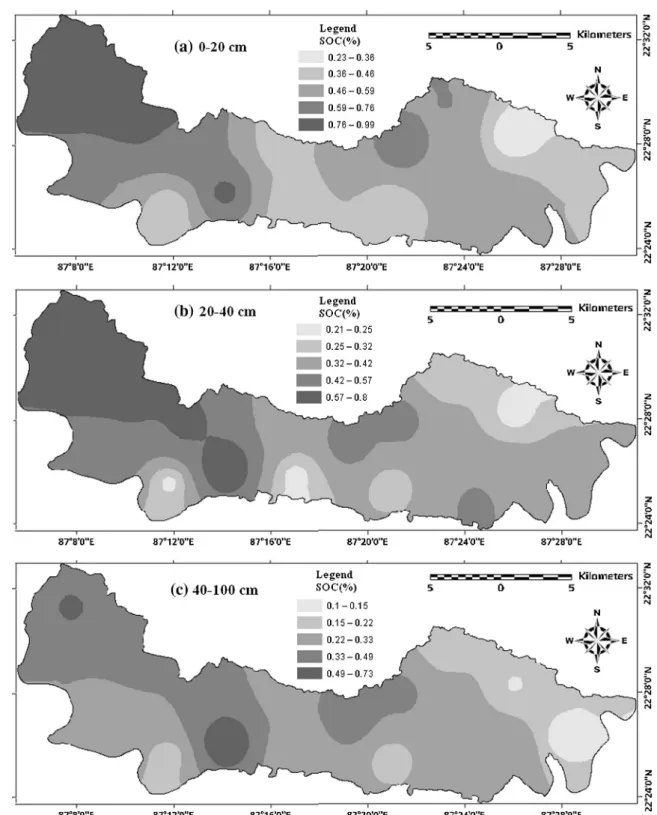
Fig. 2 represents the distribution of SOC at 0–20 cm (dark shed), 20–40 cm (dark to gray shed) and 40–100 cm (very light gray shed) depth analysis. The result showed concentration of SOC is maximum in agricultural land at 0–20 cm depth and the minimum percent was recorded in fallow land and forest (Fig. 2). Consequently, SOC percent was higher in forest and agricultural land at 20–40 cm depth and minimum percent was observed in shrubs. Results also showed the highest per-cent of SOC in forest and grassland at 40–100 cm depth and
Table 1 Land Use and Land Cover (LULC).
Class name Number of pixels Area (in km2) Percent Producer accuracy (%) User accuracy (%) Kappa^
Built-up area 14,016 12.61 3.57 80.00 100.00 1.00 River/water bodies 4581 4.12 1.17 100.00 66.67 0.65 Sand 2762 2.48 0.7 100.00 66.67 1.00 Fallow land 33,664 30.29 8.58 75.00 100.00 0.65 Forest 64,377 57.93 16.41 85.71 85.71 0.84 Grassland 16,933 15.24 4.31 80.00 100.00 0.76 Agricultural land 223,339 201.01 56.91 100.00 83.33 0.78 Shrub land 87,838 29.48 8.35 83.33 100.00 1.00 Overall classification accuracy = 88.00%.
Overall kappa statistics = 0.85.
Table 2 Summary statistics of soil organic carbon (SOC, %) content in different soil horizons.
Soil depth (cm) N Mean Median Min Max SD CV (%) Skewness Kurtosis 0–20 32 0.50 0.58 0.02 0.82 0.32 64.297 0.25 1.30 20–40 32 0.47 0.52 0.05 0.87 0.39 81.79 0.02 1.59 40–100 32 0.43 0.45 0.08 0.99 0.32 75.06 0.11 0.81 N = Number of samples, Min = Minimum, Max = Maximum, SD = Standard Deviation, CV = Coefficient of Variation.
lowest percent was observed in fallow land and agricultural land. The storage capacity of carbon among the entire forest category under consideration was significantly higher in the top layer (P< 0.03). The present result is corroborated with previous studies by Gurumurthy et al. (2009), Sheikh et al. (2011)andSaha et al. (2012).
3.3. Vertical distribution of SOC
The vertical distribution of SOC percent was analyzed (Table 2). The average value of SOC was 0.50 at 0–20 cm depth, and the percent decreased with the increase of depth (Table 2).
The skewness and kurtosis coefficients are often used to describe the shape and flatness of data distribution respectively. All the data showed positive skewness, showing the concentra-tion at lower end of data distribuconcentra-tion. SOC content ranged from 0.02% to 0.82% (0–20 cm depth) and the allocation was positively skewed due to few high values found in the western part of the area. Average SOC content was 0.47% and 0.43% at 20–40 cm and 40–100 cm depth respectively. The results also showed positive skewness. Briefly, a good concentration of car-bon sink was found in the 0–40 cm depth in all the forest soil samples in the study site. Storage of SOC in upper soil layer has been associated with the growth of root systems (Pillon, 2000) and with the quantity of aboveground biomass addition
Figure 2 Characteristics of soil organic carbon in different land use categories. The error bars represent ± one standard error.
Table 3 Comparison of the efficiencies and errors of the interpolation methods to predict SOC.
Interpolation type Interpolation method Soil depth (cm) Efficiency Error
R2 RMSE ME MRE Deterministic IDW 0–20 0.776 0.125 0.568 0.214 20–40 0.791 0.121 0.385 0.254 40–100 0.808 0.145 0.645 0.210 LPI 0–20 0.792 0.130 0.398 0.228 20–40 0.816 0.127 0.257 0.251 40–100 0.851 0.148 0.468 0.216 RBF 0–20 0.742 0.176 0.845 0.268 20–40 0.765 0.159 0.681 0.289 40–100 0.781 0.147 0.754 0.275 Geostatistical OK 0–20 0.918 0.110 0.110 0.158 20–40 0.921 0.120 0.124 0.195 40–100 0.938 0.123 0.121 0.154 EBK 0–20 0.879 0.128 0.351 0.245 20–40 0.848 0.127 0.364 0.235 40–100 0.895 0.131 0.358 0.233
R2= coefficient of determination, RMSE = root mean square error, ME = mean error, MRE = mean relative error, IDW: inverse distance weighting, LPI: local polynomial interpolation, RBF: radial basis function, OK: ordinary kriging and EB: Empirical Bayes model.
on the soil surface (Burle et al., 2005) indicating that the trees will usually increase organic carbon.
In this study, IDW, LPI, OK, EBK and RBF were used to estimate the spatial distribution of SOC. The summary statistics of the interpolation are represented in Table 3.
Fig. 3represents the spatial distribution of SOC at three differ-ent soil depth. The characteristics of the semivariograms for SOC are abridged inTable 4. Preliminary calculations showed that all semivariograms were exponential. Semivariogram analysis indicated that SOC was best fitted to exponential
Figure 3 (a) Spatial distribution of SOC using IDW (inverse distance weighting), (b) spatial distribution of SOC using LPI (local polynomial interpolation), (c) spatial distribution of SOC using BRF model (radial basis function), (d) spatial distribution of SOC using EBK (Empirical Bayesian Kriging), and (e) spatial distribution of SOC using OK (ordinary kriging).
model with nugget, sill, and nugget/sill equal to 0.15, 1.10, and 0.14, respectively for 0–20 cm depth. The value of nugget, sill, and nugget/sill was recorded as 0.001, 0.97 and 0.10 respec-tively for 20–40 cm, and 0.001, 1.08 and 9.26 for 40–100 cm soil depth respectively.
3.4. Comparison of deterministic methods
Spatial distributions of SOC were analyzed in the study area obtained by deterministic methods (IDW, LPI, and RBF). The comparative results showed LPI is more accurate than
the other two methods. The R2 value for LPI varied from 0.792, 0.816 and 0.851 for 0–20 cm, 20–40 cm and 40–100 cm respectively. TheR2value for IDW varied from 0.776, 0.791, and 0.808 for 0–20 cm, 20–40 cm and 40–100 cm respectively. However, the value of RBF showed lesser accuracy in the esti-mation method.
Most quantitative comparison of these three techniques was obtained through cross-validation statistics (Table 3).
LPI showed RMSE of 0.125, 0.121, and 0.145 at 0–20 cm,
20–40 cm and 40–100 cm soil depth respectively. IDW resulted RMSE of 0.121–0.145 whereas RBF gave RMSE of 0.147– 0.176 at different depth of SOC concentration. IDW resulted in ME of 0.385–0.645 whereas LPI gave ME of 0.257–0.468. LPI resulted in MAE of 0.216–0.251 and IDW gave RSS of 0.210–0.254. However, the result of the analysis represented that LPI is more accurate than IDW with lesser ME and smal-ler RMSE value. The analysis also showed IDW providing bet-ter result than RBF.
3.5. Comparison of geostatistical methods
The ordinary kriging (OK) and Empirical Bayes model (EBK) are used to interpolate the spatial variability of SOC in three
soil depths (Table 3). The summary results processed by OK showed the smallest RMSE value of 0.148, 0.120 and 0.123 at 0–20 cm, 20–40 cm and 40–100 cm soil depth respectively. The Coefficient of determination (R2) of the model represented
as 0.918, 0.921 and 0.938 at 0–20 cm, 20–40 cm and 40–100 cm soil depth respectively.Table 4represents the key parameters of semivariogram model for OK.
TheR2of the model at each soil depth were greater than 0.5, indicating a good fit with the ground value. OK resulted in RMSE 0.110–0.123 whereas EBK gave 0.127–0.131. The RSS was approximately close to zero for all soil depths and
it is determined that theoretical models of SOC well reflect the spatial distribution and also corresponded strongly to the spatial correlation. OK showed the ME of 0.110–0.124 whereas EBK gave 0.351–0.364. The best results, in terms of cross validation, are achieved by OK which gave the lowest RMSE, ME and MAE. The information derived from semivariograms pointed out the reality of different spatial
dependence for collected soil properties from the field (Table 4). The proportion of nugget to sill (C0/C0+C)
imi-tates the spatial autocorrelation (Wei et al., 2008).
3.6. Comparison of geostatistical and deterministic methods
The best models from the deterministic and geostatistical methods were compared to find the most suitable spatial inter-polation method of the region. Assessment measures of model performance are summarized in Table 3. The superiority of IDW, LPI, OK and EBK models over RBF to predict SOC at three different soil depths was well established. To quantify the relative performance, the percentage improvement of IDW, LPI, OK and EBK over RBF was also calculated. The obtained results are shown inTable 5and it was clearly indi-cated that IDW, LPI, OK and EB average decreased RMSE value of 18.08%, 15.65%, 26.12% and 19.93% respectively lower than RBF. Similarity reduction of MRE value of IDW, LPI, OK and EB was 18.63%, 16.51%, 39.19% and 14.18% respectively. The R2 value of IDW, LPI, OK and EBK models showed increase of 3.81%, 6.45%, 21.40%, and 14.63% over RBF model.
High value of coefficients of determination, and low value of RMSE and ME indicated a good match between observed and predicted SOC concentration at three different soil depths. The OK gave the lowest error (RMSE value) and highestR2
value in the spatial interpolation of three soil depths among all geostatistical methods. IDW and LPI methods gave the best results among the deterministic methods. Overall the perfor-mance of the geostatistical methods was thoroughly compared with that of the deterministic methods. The ordinary kriging was found the best among all of the methods. OK and related geostatistical techniques incorporate spatial autocorrelation and statistically optimize the weights. OK methods often give better interpolation for estimating values at unmeasured loca-tions (Burgess and Webster, 1980; Liu et al., 2006; Nayanaka et al., 2010; Zhang et al., 2011; Mousavifard et al., 2012;
Varouchakis and Hristopulos, 2013; Venteris et al., 2014; Tripathi et al., 2015). Among the five interpolation methods, the performance of OK was best in comparison with other interpolation models. The MRE, which provided relative error of the predicted data in reference to the actual data, was also very low for OK.
4. Conclusion
The clear understanding of SOC distribution is the key issue for agricultural and environment management. Due to relative profusion of a variety of methods, many algorithms are pre-sently applied, and research continues, aiming at the definition of the ‘‘best”method for delineation of spatial distribution of SOC. The methods are evaluated using efficiency and error estimates of interpolation techniques. The efficiency is assessed by coefficient of determination (R2value), and errors are rep-resented by the root mean square error (RMSE), mean error (ME) and mean relative error (MRE). The study shows that OK interpolation method is superior than geostatistical and deterministic methods. The performance of the exponential semi-variogram model is outstanding with OK interpolation techniques. IDW skill has the worst presentations, deriving higher RMSE and MRE than other deterministic and geosta-tistical methods. The study carries out at only 36 soil sampling sites over the study area of 353 km2
. The interpolation could be more accurate, with more close samples and incorporation of sufficient topographical information. Finally, the results guide to the amplification of trustworthy SOC concentration maps which can significantly contribute to proper application of agricultural and ecological modeling.
Acknowledgments
We extend our thanks to the Department of Geography and Environment Management, Vidyasagar University, Medinipur-721102, India, for providing necessary facilities
Table 5 Summary of the performance of interpolation methods in terms of improvement over radial basis function method.
Performance soil depth (cm) Reduction in RMSE over RBF (%) Reduction in MRE over RBF (%) Increase inR2over RBF (%) IDW LPI OK EBK IDW LPI OK EBK IDW LPI OK EBK 0–20 28.98 26.14 37.5 27.28 20.14 14.93 41.05 8.58 4.58 3.74 23.72 18.46 20–40 23.9 20.13 24.53 20.13 12.11 13.15 32.53 18.69 3.40 6.67 20.39 10.85 40–100 1.37 0.69 16.33 10.89 23.64 21.45 44.00 15.27 3.46 8.96 20.10 14.60 Average 18.08 15.65 26.12 19.43 18.63 16.51 39.19 14.18 3.81 6.45 21.40 14.63
R2= coefficient of determination, RMSE = root mean square error, ME = mean error, MRE = mean relative error, IDW: inverse distance weighting, LPI: local polynomial interpolation, RBF: radial basis function, OK: ordinary kriging, and EB: Empirical Bayes model.
Table 4 Summary of semivariogram parameters of best-fitted theoretical model to predict soil properties and cross-validation statistics.
Soil depth (cm) Best-fit model Nugget (C0) Sill (C0+C) Range (m) Nugget/sill R2 RSS ME RMSE 0–20 Exponential 0.15 1.10 1.076 0.14 0.918 0.005 0.110 0.110 20–40 Exponential 0.001 0.97 1.33 0.10 0.921 0.008 0.124 0.120 40–100 Exponential 0.001 1.08 1.21 9.26 0.938 0.003 0.121 0.123
for conducting the research work. And also we thank Raha-man Agri Clinic and Agri Business Center, Daspur (Paschim Medinipur), for providing necessary laboratory facilities for soil test.
References
Agrawal, O.P., Rao, K.V.G.K., Chauhan, H.S., Khandelwal, M.K., 1995. Geostatistical analysis of soil salinity improvement with subsurface drainage system. Trans ASAE 38, 1427–1433.
Bao, S.D., 2000. Soil and Agricultural Chemistry Analysis. China Agriculture Press, Beijing, p. 495.
Behera, S.K., Shukla, A.K., 2015. Spatial distribution of surface soil acidity, electrical Conductivity, soil organic carbon content and exchangeable Potassium, calcium and magnesium in some cropped acid Soils of India. Land Degrad. Dev. 26, 71–79.
Burgess, T.M., Webster, R., 1980. Optimal interpolation and isarith-mic mapping of soil properties I: the semivariogram and punctual kriging. J. Soil Sci. 31, 315–331.
Burle, M.L., Mielniczuk, J., Focchi, S., 2005. Effect of cropping systems on soil chemical characteristics, with emphasis on soil acidification. Plant Soil 190, 309–316.
Cambardella, C.A., Moorman, T.B., Novak, J.M., Parkin, T.B., Karlen, D.L., Turco, R.F., Konopka, A.E., 1994. Field-scale variability of soil properties in central Iowa soils. Soil Sci. Soc. Am. J. 58, 1501–1511.
Cheng, X.F., Xie, Y., 2009. Spatial distribution of soil organic carbon density in Anhui Province based on GIS. Sientia Geograph. Sin. 29 (4), 540–544 (in Chinese).
ESRI, 2001. Using ArcGIS Geostatistical Analyst. ESRI Press, Redlands, CA.
Gurumurthy, K.T., Kiran, Kumar M., Prakasha, H.C., 2009. Changes in physic–chemical properties of soils under different land use systems. Karnataka J. Agric. Sci. 22 (5), 1107–1109.
Hani, A., Abari, S.A.H., 2011. Determination of Cd, Zn, K, pH, TNV, organic material and electrical conductivity (EC) distribution in agricultural soils using geostatistics and GIS (case study: South Western of Natanz – Iran). World Acad. Sci., Eng. Technol. 5 (12), 22–25.
Hussain, I., Shakeel, M., Faisal, M., Soomro, Z.A., Hussain, T., 2014. Distribution of total dissolved solids in drinking water by means of Bayesian kriging and gaussian spatial predictive process water quality. Expos. Health 6 (4), 177–185.
Johnston, K., Ver, Hoef J.M., Krivoruchko, K., Lucas, N., 2001. Using ArcGIS Geostatistical Analyst. ESRI Press, Redlands, CA. Knotters, M., Heuvelink, G.B.M., Hoogland, T., Walvoort, D.J.J., 2010. A Disposition of Interpolation Techniques; Wageningen University and Research Centre, Statutory Research Tasks Unit for Nature and the Environment: Wageningen, The Netherlands. Krivoruchko, K., 2012. Empirical Bayesian Kriging. Esri, Redlands,
CA, USA. Available online: <http://www.esri.com/news/arcuser/ 1012/empirical-byesian-kriging.html> (accessed 17.10.15). Krivoruchko, K., Butler, K., 2013. Unequal Probability-Based Spatial
Mapping. Esri, Redlands, CA, USA. Available online: <~/media/ Files/Pdfs/news/arcuser/0313/unequal.pdf" xlink:type="simple" id="ir010">http://www.esri.com/esrinews/arcuser/spring2013/
~/media/Files/Pdfs/news/arcuser/0313/unequal.pdf>.
Kumar, S., Lal, R., Liu, D., Rafiq, R., 2013. Estimating the spatial distribution of organic carbon density for the soils of Ohio, USA. J. Geogr. Sci. 23 (2), 280–296.
Kumar, S., Lal, R., Lloyd, D.C., 2012. Assessing spatial variability in soil characteristics with geographically weighted principal compo-nents analysis. Comput. Geosci. 16, 827–835. http://dx.doi.org/ 10.1007/s10596-012-9290-6.
Li, X.F., Chen, Z.B., Chen, H.B., Chen, Z.Q., 2011. Spatial distribu-tion of soil nutrients and their response to land use in eroded area of South China. Proc. Environ. Sci. 10, 14–19.
Li, Y., Shi, Z., Wu, C.F., Li, H.X., Li, F., 2007. Improved prediction and reduction of sampling density for soil salinity by different geostatistical methods. Agric. Sci. China 6, 832–841.
Liu, D., Wang, Z., Zhang, B., Song, K., Li, X., Li, J., 2006. Spatial distribution of soil organic carbon and analysis of related factors in croplands of the black soil region, northeast China. Agric. Ecosyst. Environ. 113, 73–81.
Liu, L., Wang, H., Dai, W., Lei, X., Yang, X., Li, X., 2014. Spatial variability of soil organic carbon in the forestlands of northeast China. J. Forest. Res. 25 (4), 867–876.
Mirzaei, R., Sakizadeh, M., 2015. Comparison of interpolation methods for the estimation of groundwater contamination in Andimeshk–Shush Plain Southwest of Iran. Environ. Sci. Pollut. Res., 1–12
Mousavifard, S.M., Momtaz, H., Sepehr, E., Davatgar, N., Sadaghi-ani, M.H.R., 2012. Determining and mapping some soil physico– chemical properties using geostatistical and GIS techniques in the Naqade region, Iran. Arch. Agron. Soil. Sci. http://dx.doi.org/ 10.1080/03650340.2012.74055.
Nayanaka, V.G.D., Vitharana, W.A.U., Mapa, R.B., 2010. Geosta-tistical analysis of soil properties to support spatial sampling in a paddy growing Alfisol. Trop. Agric. Res. 22, 34–44.
Nielsen, D.R., Wendroth, O., 2003. Spatial and Temporal Statistics— Sampling Field Soils and Their Vegetation. Catena Verlag GMBH, Reiskirchen, German.
Pang, S., Li, T.X., Zhang, X.F., Wang, Y.D., Yu, H.Y., 2011. Spatial variability of cropland lead and its influencing factors: a case study in Shuangliu county, Sichuan province, China. Geoderma 162, 223–230.
Pillon, C.N., 2000. Stocks and Quality of soil Organic Matter as Affected by No –Till Cropping System, Doctorate Thesis. Federal University of Rio Grande do Sul, Porto Alegre, pp. 248.
Robertson, G.P., 2008. GS+: Geostatistics for the Environmental Sciences. Gamma Design, Plainwell, Mich..
Robinson, T.P., Metternicht, G.M., 2006. Testing the performance of spatial interpolation techniques for mapping soil properties. Comput. Electeron. Agric. 50, 97–108.
Saha, D., Kukal, S.S., Bawa, S.S., 2012. Soil organic carbon stock and fractions in relation to land use and soil depth in the degraded shiwaliks hills of lower Himalayas. Land Degrad. Dev.http://dx. doi.org/10.1002/ldr.2151.
Saito, H., McKenna, A., Zimmerman, D.A., Coburn, T.C., 2005. Geostatistical interpolation of object counts collected from multi-ple strip transects: ordinary kriging versus finite domain kriging. Stoch. Environ. Res. Risk Assess. 19, 71–85.
Sheikh, A.M., Kumar, M., Bussman, R.W., Todari, N.P., 2011. Forest carbon stocks and fluxes in physiographic zones of India. Carbon Bal. Manage. 6 (15), 1–10.
Shit, P.K., Bhunia, G.S., Maiti, R.K., 2013. Assessment of factors affecting ephemeral gully development in badland topography: a case study at Garbheta badland (Pashchim Medinipur). Int. J. Geosci. 4 (2), 461–470. http://dx.doi.org/10.4236/ijg.2013. 42043.
Soil Survey Manual, 1970. All India Soil and Land Use Survey Organization. I.A.R.I., New Delhi.
Tripathi, R., Nayak, A.K., Shahid, M., Raja, R., Panda, B.B., Mohanty, S., Kumar, A., Lal, B., Gautam, P., Sahoo, R.N., 2015. Characterizing spatial variability of soil properties in salt affected coastal India using geostatistics and kriging. Arab. J. Geosci.
http://dx.doi.org/10.1007/s12517-015-2003-4.
Varouchakis, E.A., Hristopulos, D.T., 2013. Comparison of stochastic and deterministic methods for mapping groundwater level spatial variability in sparsely monitored basins. Environ. Monit. Assess. 185, 1–19.
Vauclin, M., Vieira, S.R., Vachaud, G., Nielsen, D.R., 1983. The use of cokriging with limited field soil observations. Soil Sci. Soc. Am. J. 47, 175–184.
Venteris, E., Basta, N., Bigham, J., Rea, R., 2014. Modeling spatial patterns in soil arsenic to estimate natural baseline concentrations. J. Environ. Qual. 43 (3), 936–946.
Wang, Y.Q., Shao, M.A., 2013. Spatial variability of soil physical properties in a region of the Loess Plateau of PR China subject to wind and water erosion. Land Degrad. Dev. 24 (3), 296–304.
Wei, J.B., Xiao, D.N., Zeng, H., Fu, Y.K., 2008. Spatial variability of soil properties in relation to land use and topography in a typical small watershed of the black soil region, northeastern China. Environ. Geol. 53, 1663–1672.
Zare-mehrjardi, M., Taghizadeh-Mehrjardi, R., Akbarzadeh, A., 2010. Evaluation of geostatistical techniques for mapping spatial
distribution of soil PH, salinity and plant cover affected by environmental factors in Southern Iran. Not. Sci. Biol. 2 (4), 92–103.
Zhang, W., Wang, K.L., Chen, H.S., He, X.Y., Zhang, J.G., 2012. Ancillary information improves kriging on soil organic carbon data for a typical karst peak cluster depression landscape. J. Sci. Food Agric. 92 (5), 1094–1102.
Zhang, Z., Yu, D., Shi, X., Weindorf, D.C., Sun, Y., Wang, H., Zhao, Y., 2011. Effects of prediction methods for detecting the temporal evolution of soil organic carbon in the Hilly Red Soil Region, China, Environ. Earth Sci. 64, 319–328.http://dx.doi.org/10.1007/ s12665-010-0849-z.