Validation and optimization of analog circuits using randomized search algorithms

(1)

(2)

VALIDATION AND OPTIMIZATION OF ANALOG CIRCUITS USING RANDOMIZED SEARCH ALGORITHMS

BY

SEYED NEMATOLLAH AHMADYAN

DISSERTATION

Submitted in partial fulfillment of the requirements

for the degree of Doctor of Philosophy in Electrical and Computer Engineering in the Graduate College of the

University of Illinois at Urbana-Champaign, 2016

Urbana, Illinois

Doctoral Committee:

Associate Professor Shobha Vasudevan, Chair Professor Thenkurussi Kesavadas

Associate Professor Xin Li Associate Professor Sayan Mitra Professor Rob Rutenbar

(3)

ABSTRACT

Analog circuits represent a large percentage of the chips used in mobile com-puting, communication devices, electric vehicles, and portable medical equip-ment today. Rapid scaling and shrinking chip geometrics introduce new challenging problems in verification, validation, and optimization of analog circuits. These problems include test generation and compression, runtime monitoring and analyzing the worst-case behaviors. State of the art tech-niques in Monte Carlo are unable to address these problems effectively. Con-sequently, designing an efficient and scalable CAD algorithm to address such problems is highly desirable.

In this thesis, we introduce Duplex, a methodology for search and opti-mization. Duplex supports optimizing nonconvex nonlinear functions and functionals. We use duplex to solve problems in analog validation and ma-chine learning. Duplex uses random tree data structures. Duplex is based on partitioning and separating the problem space into multiple smaller spaces such as input, state and the function space. Duplex simultaneously controls, biases and monitors the growth of the random trees in the partitioned spaces. We have used the duplex framework to solve practical problems in analog and mixed signal validation like directed input stimuli generation, compressing analog stress tests, worst-case eye diagram analysis, performance optimiza-tion, machine learning, and monitoring runtime behaviors of analog circuits. We used Duplex for validation and optimization of analog circuits. Duplex automatically generates input stimuli that expose bugs and improves cover-age. Duplex automatically finds input corners that result in worst-case eye diagrams. Duplex simultaneously explores the parameter and performance spaces of analog circuits to optimize the circuit for best performance. We monitored the random trees and circuit execution against the specification properties described in formal languages. We formulated many challenging problems in the analog circuits, such as test compression and eye diagram

(4)

analysis, as functional optimization problems. We use Duplex to solve these functional optimization problems.

We propose the Duplex algorithm as an optimization algorithm to posit the framework to other domains. Duplex can address nonlinear and functional optimization problems in continuous and discrete spaces such as design-space exploration and supervised and unsupervised machine learning.

The advantages of the duplex framework are efficiency, scalability and versatility. We consistently show orders of magnitude speedup improvements over the state of the art while objectively improving the quality of results. For generating input stimuli, duplex is the first technique that simultaneously does directed input stimulus generation and increases test coverage. We show over two orders of magnitude speedup over Monte Carlo simulations. For runtime monitoring, we check a large scalable circuit against a very expressive set of formal properties that were not possible to monitor before. For generating worst-case eye diagram, we show at least 20_× speedup and better quality of results in comparison to the state of the art. Duplex is the first work to provide transient test compression for analog circuits. We compress stress tests up to 96%. We optimize analog circuits using Duplex and we show speedup and improved results with respect to the state of the art. We use Duplex to train supervised and unsupervised models and show improved accuracy in all cases.

(5)

ACKNOWLEDGMENTS

I would like to thank my adviser, Prof. Shobha Vasudevan, for her intellect, experience, and advice. Of all people, I owe her the most for the completion of this thesis.

I would like to thank my dissertation committee members, Prof. Rob Rutenbar, Prof. Sayan Mitra, Prof. Martin Wong, Prof. Xin Li, and Prof. Kesh Kesavadas, for their time, invaluable feedback and for agreeing to be part of my Ph.D. exam process.

I would like to also thank my co-authors and collaborators, Dr. Jayanand Asuk Kumar, Dr. Suriya Natarajan, Dr. Chenjie Gu, and Dr. Eli Chiprout, for their work, experience, and feedback.

I would like to thank my parents, who supported me all these years, my sis-ters, and friends Fardin Abdi, Hadi Hashemi, Mohammad Babaizadeh, Faraz Faghri, Mohammad Nourbakhsh, Jalal and Rasoul Etesami, and many oth-ers. Finally I would like to thank Samira Sheikhi, for her kindness, intellect, support and intriguing conversations.

(6)

LIST OF TABLES

1.1 Keystone problems in analog validation and optimization . . . 3

4.1 Performance comparison of MORRT vs M.C. . . 61

6.1 Space partitioning tree statistics. During the execution of the iterative reachable set reduction algorithms, most of the generated polytopes are at the boundaries of the reachable set and they rapidly get smaller in volume. _†

indicates that the number is a two-dimensional volume. . . 108

8.1 Parameters of the random tree . . . 143

9.1 Performance specification for the opamp circuit and the result of circuit optimization. Duplex determines the opti-mum value for the parameters and performance metrics of

the circuit. . . 161 9.2 Result of Duplex optimization of the CP-PLL circuit.

Du-plex determines the optimum value for the parameters and

(10)

LIST OF FIGURES

1.1 The overview of the problems solved in analog design flow. . . 2

1.2 Duplex solves different types of optimization problems. . . 7

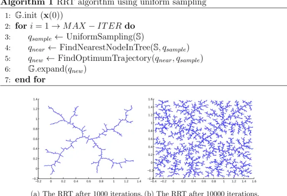
3.1 Growth of RRT through addition of a new node sampled from the state space. . . 28

3.2 The classic RRT algorithm does not have any direction or bias and rapidly explores the entire reachable state space. . . . 29

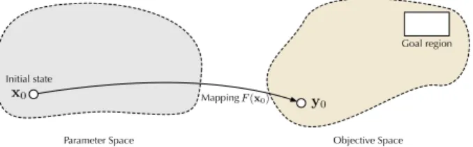
3.3 The input and objective spaces in multi-objective optimization. 33 3.4 The convergence rate w.r.t. number of iterations for the Duplex algorithm for nonconvex optimization. Our algo-rithm converges very fast toward the optimum solution from any initial state. Duplex is not sensitive to the choice of initial state. . . 35

3.5 Growing random tree toward the goal region. . . 38

3.6 The Pareto frontier of the random tree. . . 39

3.7 Using Duplex for optimizing a non-convex function. . . 42

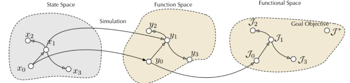
3.8 Partitioning the spaces into state space and function (ob-jective) spaces in Duplex. . . 43

3.9 The result of the Dido optimization problem using Duplex algorithm. . . 45

4.1 Framework of our directed input stimulus generation tech-nique (Section 4.2) . . . 50

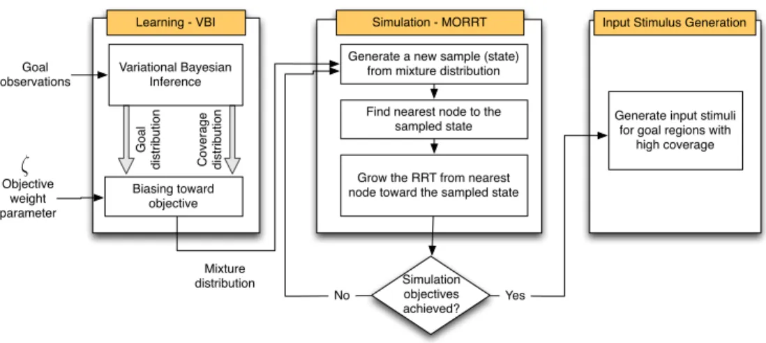
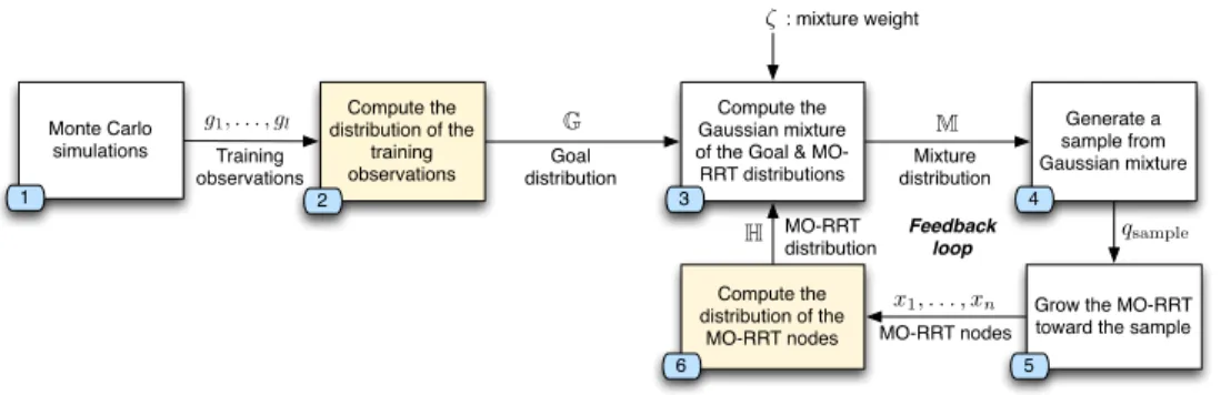
4.2 Detailed block diagram of the learning phase of the Multi-Objective RRT algorithm. First, we identify the goal dis-tribution (block 1 and 2). We grow the MORRT by sam-pling states from the mixture distribution. We feed the MORRT states back to the learning algorithm to update the mixture distribution (blocks 6 and 3). Shaded regions corresponds to the VBI algorithm. . . 52

4.3 An example of the input stimuli generated for the Joseph-son circuit (Section 4.4.1) from the MORRT. Generating input stimulus for Josephson circuit is difficult using con-ventional Monte Carlo methods. . . 58

(11)

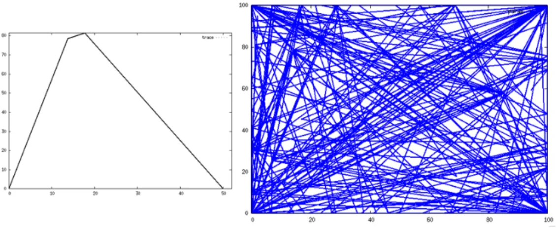
4.5 Exploring the state space of a Josephson junction circuit using the classic RRT and MORRT. Figure 4.5a shows the classic RRT algorithm; for the given number of iterations (3,000), the algorithm did not converge. Figures 4.5b to 4.5g show the various MORRT results for different increas-ing values ofζ. Finally, Figure 4.5h shows a trace extracted from our algorithm. For the same number of iterations, the MORRT algorithm will converge faster and provide more

coverage of the region around the equilibrium state (0,0). . . . 60

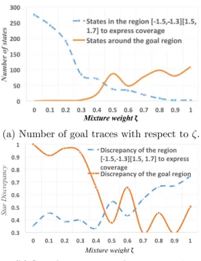
4.6 Effects ofζ on discrepancy and number of states in MORRT. . 63

4.7 Schematic of the opamp circuit. . . 64

4.8 Generating tests for stressing the resister R1 . . . 65

4.9 Combining different tests. The MO-RRT can learn the goal regions from two given test sets and generate a combined tests that simultaneously reaches both goal regions. . . 67

4.10 Combining different tests. The MO-RRT can learn the goal regions from two given test sets and generate a combined test that simultaneously reaches both goal regions. . . 68

4.11 Schematic of the VCO circuit. . . 70

4.12 Generating input stimuli for VCO circuit. . . 71

4.13 Tunnel-diode circuit. . . 71

4.14 Effect of mixture weightζ on the mixture Gaussian distri-bution M. The mixture distribution converges toward the distribution of the goal regionGfor goal-oriented MORRT with higherζ. On the other hand, a lowerζ with coverage-driven objective ensures thatM is closer the MORRT dis-tribution H. . . 72

4.15 Tunnel diode results for classic and MORRT algorithm. While the classic RRT algorithm will generate a lot of sam-ples to find its path towards two stable equilibrium points (the boxed regions), the MORRT algorithm will rapidly converge and will generate more traces in relevant regions and explores more regions of the state space. Moreover, the MORRT will provide a better coverage in the reach-able state space (the enveloped region). . . 72

4.16 Schematic of the ring modulator circuit. The ring mod-ulator consists of four parts: the input stage, the carrier stage, the output stage, and the diode ring. The circuit modulates the input signalVin with carrier signalVCarrier. . . . 73

4.17 The output of the carrier stage is relatively clean according to the specification, because of the RC filter in the design. Therefore, the output perturbation is propagated from the input stage through the diode ring. The cause of the bug in the circuit is the poor input stage filter design. . . 75

(12)

4.18 Exploring the reachable state space using MORRT. For each leaf node in the MORRT, we can extract the input sequence that will generate that trace. The VBI algorithm inferred the distribution at the origin as the goal region. As a result, most of the traces are focused around the center

of the region. . . 76

5.1 Flowchart of TRRT-based runtime monitoring algorithm. . . . 84

5.2 Tunnel-diode oscillator circuit. . . 90

5.3 Random tree outputs for tunnel diode oscillator. . . 91

5.4 Phase-locked loop (PLL) circuit . . . 92

5.5 The TRRT trace of signal deviation for a loop filter. . . 93

6.1 Overview of the iterative reachable set reduction algorithm. The exterior loop is the iterative reachable set reduction algorithm. For each polytope, our algorithm partitions it. Then, for each new partition, our algorithm decides on the reachability of those partitions from the reachable set. The parts of our algorithm that use SPT for computation are marked with SPT labels. . . 98

6.2 Partitioning a polytope based on state space trajectories. . . . 101

6.3 Determining existential positivity of the reachability deci-sion function. Our algorithm rotates the functionθdegrees to align it to the axis. Therefore, other variables become constant, and the reachability decision function becomes a single-dimensional basis function. . . 103

6.4 State space partitioning using hyperplanes. The polytopes are defined by the intersections of the hyperplanes in the state-space. . . 105

6.5 Reachable set for the Van der Pol oscillator using our itera-tive reachable set reduction algorithm. The reachable set is in grey and the unreachable states are in white. The poly-topes at the boundaries of the reachable set shrink rapidly in volume. . . 107

7.1 Eye diagram. . . 113

7.2 The high-level description of our approach. We use the eye diagram as a feedback in our approach and minimize the distortion functionals using the random tree algorithm. . . 113

7.3 The distortion functionals. . . 115

7.4 The growth of the random tree algorithm. . . 118

7.5 Schematic of CMOS inverter circuit. . . 120 7.6 The worst-case analysis of the eye diagram in Monte Carlo

vs. our algorithm. Given the same number of iterations, our algorithm generates an eye diagram that is 47% smaller

(13)

7.7 The convergence rate of random tree algorithm vs. Monte Carlo for the eye diagram analysis. The random tree

algo-rithm converges much faster that Monte Carlo. . . 122 7.8 The size of the eye diagrams for different maximum

devia-tions for simulation parameters. . . 122 7.9 The scatter plot of the VDD inputs for generating the

fron-tier set s1. The left side figure shows the histogram of the

VDD inputs samples (we excluded the samples from the ideal path). The right side is the scatter plot of input stimuli drawn over time, which identifies three separate

component in the worst-case eye diagram. . . 124 7.10 The eye diagram of ring oscillator circuit computed using

our technique. . . 125

8.1 Compressed test z with the optimal time among all

func-tionally equivalent tests_{x, y, z_}. . . 128 8.2 The modeling of the test compression problem. . . 132 8.3 Contradiction test with minimum time but not minimum

flux functional. . . 133 8.4 Generalization of the proof to higher dimensions. . . 133 8.5 Random tree algorithm to minimize flux functional. . . 135 8.6 We use the inverter circuit as an illustrative example for

test compression. . . 137 8.7 The flowchart of the greedy algorithm for compress test in

the presence of process variation. . . 139 8.8 Parallel version of the random tree algorithm to minimize

flux functional. The SPICE simulations are executed

con-currently. . . 142 8.9 Schematic of the operational amplifier circuit. . . 143 8.10 Saturation test for the opamp circuit. . . 144 8.11 Using random trees to compress stress tests for circuit’s

components. . . 144 8.12 Compression ratio for different tests. . . 145 8.13 Combining different tests. . . 146 8.14 Compressing tests for VCO circuit. Our technique

com-pressed VCO swing tests by 88%. . . 147 8.15 Process variation in the width of NMOS and PMOS

tran-sistors in the inverter circuit and worst-case corner. . . 147

9.1 Schematic of an inverter circuit that we use as an illustra-tive example. We want to optimize the width of NMOS

and PMOS transistors to minimize dynamic power and delay. 153 9.2 The relation between constrained parameter space (left)

and the reachable performance space and the goal region

(14)

9.3 Flowchart of the Duplex random tree search algorithm for

performance optimization. . . 154 9.4 Growing parameter and performance tree in the parameter

and performance space. . . 155 9.5 Schematic of a two-stage operational amplifier. . . 161 9.6 Using Duplex for optimizing the bandwidth of the op-amp. . . 162 9.7 The convergence rate w.r.t. number of iterations for the

Duplex algorithm for the inverter case study. Our algo-rithm converges very fast toward the optimum design from any initial state. Duplex is not sensitive to the choice of

initial state. . . 163 9.8 The sensitivity graph visualizing performance to parameter

sensitivity for opamp case-study.The Edges are annotated with the sensitivity of a performance metric (a node in the

right side) to a particular parameter (a node on the left side). 164 9.9 Distribution of the optimal parameters for the opamp

cir-cuit. Duplex computes the Pareto set as a mixture Gaus-sian distribution by inferring the distribution of the sam-ples in the goal region. Pareto surface is computed from the CDF of the pareto distribution. We use the mean of

the distribution as the optimum state. . . 165 9.10 Schematic of a post-layout charge-pump PLL circuit. . . 166

10.1 Duplex algorithm cluster samples together by minimizing

the distortion function. . . 170 10.2 Duplex algorithm cluster samples together by minimizing

(15)

CHAPTER 1 INTRODUCTION

1.1 Design automation for analog circuits

Analog circuits represent a large percentage of the chips used in mobile com-puting, communication devices, electric vehicles, and portable medical equip-ment today [1]. This trend is projected to grow in the future [1], as analog IPs become ubiquitous in SoC designs. The analog IP market is expected to expand with the increasing demand for portable and wearable devices, smart-phones, and low-power electronics [1]. Analog chips are increasingly being used in medical devices and electric vehicles [1], where safety and reliability are critical concerns.

Verification and validation of the behavior of these complex and safety crit-ical circuits is a daunting challenge. The scale and complexity of the circuits have increased significantly beyond those of the hand-crafted, isolated analog circuits of the past. However, given the scale and complexity of the analog components used in modern devices, traditional validation methodologies based on Monte Carlo simulations are inefficient, expensive, error-prone, and frequently misleading in predicting unknown behaviors, worst case corners and stressing weak components of the circuit. It is critical to automate the validation tasks for analog circuits to meet demands [2].

1.1.1 Fast and reliable circuits

Analog circuits are the drivers of the computer and electronics industry. Circuits are manufactured at a very large scale at a very low margin. In this competitive market, analog designers always strive to design reliable chips with maximum performance. It is crucial to vigorously test against design errors to ensure reliability, correctness, and safety.

(16)

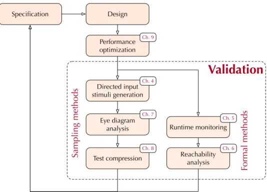
Specification Design Runtime monitoring Reachability analysis Directed input stimuli generation Eye diagram analysis Performance optimization Test compression Ch. 9 Ch. 4 Ch. 5 Ch. 6 Ch. 7 Ch. 8

Validation

Formal methods Sampling methods

Figure 1.1: The overview of the problems solved in analog design flow.

through the cycle of specification → design → optimization→ vali-dation. Currently every task in analog validation is manual and ad-hoc. As a result, the analog design process is error-prune, expensive and very time-consuming. Our mission is to provide automation in analog design flow to improve the quality and reliability of analog circuits. In particular, we focus on optimization and validation of analog circuits.

Validation: We define the validation problem in analog circuits as ensur-ing the circuit is behavensur-ing correctly accordensur-ing to its specification. An analog circuit is a nonlinear system with input and output signals. For validating such regime, two categories of problems arise. Firstly, how to excite the in-put; how to generate meaningful input stimuli to test the circuit. We wish to generate tests that trigger failures, bugs, or worst-case responses in the circuits. Secondly, how to monitor the output response, check for violations, and ensure the safety of the circuit.

The goal of exciting the inputs to identify input stimuli and corners that can cause failure in the circuit. Failures can be viewed as having a failed state (such as signal cut-off, unstable output, failure to lock, etc.) or noisy output (jitter, weak signal, low noise margin, etc.). Then we can analyze the generated input stimuli to discover bugs in the design and improve the circuit.

(17)

Table 1.1: Keystone problems in analog validation and optimization

Type Chapter Problem

Validation 4 Directed input stimuli generation

Validation 5 Runtime monitoring and property checking

Validation 7 Worst-case eye diagram and signal-integrity analysis Optimization 8 Test compression

Optimization 9 Performance optimization of analog circuits Validation 6 Reachability analysis and safety verification

Finally, During test and after finding the test stimuli, we can optimize it such that the test would be executed faster on the circuit in order to save time (Chapter 8).

For ensuring the safety and correctness of the circuit, we can take either a universal or existential approach. In the universal approach, we have to prove the circuit is correct by verifying every possible execution meets the specification. One universal tool for verifying safety properties is reachability analysis (Chapter 6). On the other hand, the existential method looks for circuit traces that violate the specification and cause failures. In order to implement the existential technique we need techniques that actively search for violating stimuli (Chapter 4 and 7) and monitor the executions (Chap-ter 5). The analog circuits exhibit complex nonlinear dynamics and have a large scale with hundreds of dimensions. Any method for validating analog circuits has to be scalable and faithful to the nonlinearities of the circuit.

Optimization: The circuit’s performance metrics include power, band-width, gain, etc. The goal of the optimization step is to improve the per-formance without changing the functionality of the circuit. We optimize the circuit’s parameters, such as transistor width and length, to improve the performance (Chapter 9).

In this thesis, we address all of the above issues in analog validation and optimization by solving six keystone problems as shown in Table 1.1. To address these significant problems in analog EDA, we need a new scalable, efficient, versatile, mathematically sound and unified methodology to replace the old techniques.

(18)

1.2 Duplex methodology

We introduce Duplex, an optimization methodology to solve non-convex and functional optimization problems. We use Duplex to solve validation and optimization problems in analog. Our methodology is based on formulating analog problems as optimization problems, then using Duplex to optimize the objective function and determine the optimum solution. The optimum solutions depend on the problem and range from the input stimuli that will cause the circuit to fail, to the worst-case eye diagram, to the optimum parameters for optimizing the circuit.

Duplex can solve three types of optimization problems: i) state-based search, ii) non-convex optimization, and iii) functional optimization. Au-tomated input stimuli generation is formulated as a state-based search prob-lem. Performance optimization is formulated as a non-convex optimization problem. Finally, eye diagram analysis and test compression problems are formulated as functional optimization problems. The overview of the Duplex methodology is shown in Figure 1.2.

The Duplex idea is centered around growing random tree structure in the space model of the problem. Depending on the problem type, Duplex algo-rithm partitions the problem space into the input space, the output space, and the function space. We simultaneously search and grow multiple mir-rored random trees in these spaces to meet the boundary conditions and optimize the objectives.

The principle of Duplex is different from other known optimization algo-rithms like simulated annealing [3], gradient descent [4], etc., used in opti-mization. Duplex simultaneously analyzes and partitions the problem space into smaller spaces such as input (feature), output (objective) and function spaces. Global decisions are made in the objective space and actions are taken locally in the input space. In every iteration, Duplex identifies the best strategy to get closer to the goal region (the optimum solution) and takes the appropriate action within the input space. The algorithm then passes the control back to the objective space, where the next such strategic decision is made. To the best of our knowledge, this is the first algorithm to simultaneously keep track of an objective/goal and use it to guide local steps.

(19)

Duplex provides valuable feedback to the user by looking at and analyzing the grown tree in the state space. Duplex uses the random tree to determine the Pareto frontier and the optimum solutions. Furthermore, Duplex avoids getting stuck in the local minima. We utilize these properties of Duplex to generate a Pareto optimal set of the circuit’s parameters in circuit opti-mization problem and analyze the distribution of worst-case samples in eye diagram analysis.

1.2.1 Advantages of the Duplex methodology

Duplex algorithm provides the following advantages over traditional opti-mization methods such as gradient descent and Newton optiopti-mization:

• Convergence guarantees toward global optimum: Optimization algorithms traverse the state space locally. They walk in the state space linearly along the direction of the gradient. Therefore, they have no notion of the solution, or where it might lie. They are prone to getting stuck in local minima and saddle points where the gradient is zero. However, Duplex performs an open ended search only in the objective space. In the objective space, it uses the basic random tree search to find the globally optimal design or the goal region. In the state space, it decides which parameter needs to change to get closer to the goal region. This decision is made using a noisy gradient descent algorithm in combination with reinforcement learning that evaluates the history of previous changes to the parameters in the parameter tree based on a reward function. There is no open ended search in the parameter modification phase (local step) of the algorithm. Duplex grows multiple different branches toward the goal state. If one of those branches gets stuck in local minima, the algorithm can branch from another state and make forward progress toward the goal. Due to the probabilistic completeness property of random trees, Duplex does not get stuck in local minima. This is in contrast to random walk based methods like simulated annealing or gradient descent. The guidance in every step from the global search towards the local step decision helps in converging quickly to the optimal goal region.

(20)

• Performance Efficiency: A search based optimization algorithm like Duplex has a benefit over classical optimization algorithms in being able to keep track of the global picture (goal states) and react with local actions. Random trees are shown to consistently outperform random walk based search methods such as Monte Carlo simulations for search applications. The improvement in efficiency is partly due to the tree data structure maintained by the random tree algorithm during the simulation. While growing, it samples a new state in the goal region (desired solution set), and then determines which state is closest (in L2-norm sense) to that sampled goal state among all of the previously

visited states in the tree. It simulates a path between the closest state and the newly sampled state and adds the new state to the tree. This is in contrast to the memory-less sampling of points in the Monte Carlo based methods. The branching to any previously visited state makes convergence to the solution set quicker than memory-less methods due to the versatility in paths traversed.

• Scalability: A tradeoff in search based algorithms comes from the step where they search for their nearest neighbors. Searching for the nearest neighbors in the state space (which scales) can be very expen-sive. Duplex addresses this issue by separating the objective functions from the state space and limiting the search for nearest neighbors only to the objective functions. The space of objective functions is much smaller than the state space, helping the scale and efficiency of Duplex significantly.

1.3 Analog problems solved with Duplex

We achieve our mission by using Duplex methodology for verification, vali-dation and optimization of analog circuits. We use the Duplex methodology to automate keystone problems in analog optimization and validation. Fig-ure 1.2 shows the flowchart of analog design flow using the Duplex method-ology. We solved select challenging problems in analog design flow.

Specifically, we use Duplex for state search, non-convex and functional op-timization in order to address problems in directed input stimuli generation (Chapter 4), worst-case eye diagram analysis (Chapter 7) and test

(21)

compres-Duplex Algorithm

State optimization Non-convex _optimization _optimizationFunctional

Eye diagram analysis Test

compression Performance

optimization Machine learning Directed input stimuli generation Runtime monitoring Reachability analysis Ch. 9 Ch. 4 Ch. 5 Ch. 6 Ch. 10 Ch. 8 Ch. 7

Figure 1.2: Duplex solves different types of optimization problems.

sion (Chapter 8). We use Duplex for design-space exploration of analog circuits to determine the optimum configuration and optimize the circuit’s performance (Chapter 9). We monitor the growth of random trees to falsify logical properties (Chapter 5) or verify safety properties by reachability anal-ysis (Chapter 6). Beyond analog, we use Duplex in machine learning to solve problems in classification and clustering where we use Duplex to optimize the loss/cost/error/energy function (Chapter 10).

1.3.1 Validating analog circuits by generating directed input

stimuli

Directed input stimuli generation

Validating nonlinear analog circuits is a major challenge and an ongoing topic of intensive research. Simulation-based verification is performed using several test cases for the circuit. Each test case is a sequence of values that is applied to the circuit inputs. For each test case, the circuit is simulated by applying the corresponding sequence of values to the inputs. The behavior induced by these sequences is then analyzed. If an erroneous or illegal set of circuit states (i.e., a ”bad” region) is known, it is desirable to check whether there is a legal sequence of input values that takes the circuit from an ini-tial state to the bad region. Simulation-based verification is non-exhaustive and therefore checks only a subset of all possible behaviors. The quality of simulation-based verification is determined by the choice of test cases.

We use Duplex for directed input stimuli generation for analog circuits. We use a learning-based approach to guide the Duplex algorithm towards a goal region. Duplex can search the state space for multiple objectives such

(22)

as reaching a goal region and improving the coverage of the state space.

We present the first technique for directed input stimuli generation for analog circuits. Duplex can generate tests with multiple objectives such as reaching a goal region and improving the coverage of the state space. Duplex can find input stimuli that trigger failures two orders of magnitude faster than Monte Carlo.

Worst-case eye diagram generation In many RF applications and driver circuits the signal integrity is crucial for the performance of the cir-cuit. Signal integrity is the major bottleneck to the system’s performance in a high speed CMOS circuit. Eye diagrams [5] are the main diagnostic technique for evaluating the signal integrity. Important signal properties such as noise margin and jitter can be measured from the eye diagram us-ing Monte Carlo transient simulations [6], statistical methods [7],[8], and analytical convolution-based techniques [9],[10].

The worst-case eye diagram is a geometric product of the distortion in the transient response of the circuit. Using Duplex, we optimize the distortion in circuit’s response my controlling the circuit’s inputs and finding the worst-case input.

We verify the signal integrity of analog circuits by analyzing the eye dia-grams. We generate worst-case eye diagrams using Duplex. Duplex is 20_×

faster than Monte Carlo based simulation and provides reasoning why the circuits is under-performing as a feedback for the user.

Optimizing input stimuli for compressing analog tests:

With the movement towards system-on-chip (SoC) ICs, the number and di-versity of mixed-signal circuits on a die has increased significantly in the form of different high-speed IOs, sensors, power, and clocking circuitry. Among these, analog components are tested using specification-based functional tests with some design-for-test (DFT) features built in.

The steps in manufacturing test are broadly categorized into wafer/sort testing, packaged part class test (using functional and structural tests) which includes stress testing/burn-in, and system testing [11]. These steps need to be performed on every part that is shipped, resulting in a high volume of parts to be tested. To achieve fast product ramp to customers, the test time per part should be small, to the order of a few seconds. Although short test times can be achieved by increasing the test equipment, this is not a preferred choice due to the sharp increase in capital cost that accompanies it. Instead,

(23)

it is cost effective to abbreviate each step in the testing of parts [11] so that the test time is reduced for each part. While the steps themselves cannot be eliminated due to the coverage they provide, reduction of time in each step is the best resort. Since every step usually provides some incremental coverage, reduction of time in each step is usually resorted to, rather than eliminating a step itself.

Reducing the cost of production test has been a topic of intense research in analog testing [11]. There are three approaches to reduce test time: i) optimal ordering of the tests, where the most failed tests are strategically placed first in order to reduce the total test time [12, 13], ii) selecting the subset of the tests to achieve the same coverage [14, 15], iii) automated development of better and more efficient tests that provide more coverage [16]-[17] and, iv) reducing the communication time by compressing tests on-chip [18, 19]. To the best of our knowledge, no previous work in analog domain has addressed the problem of reducing each individual test’s time.

We formulate the test compression problem as an optimization problem. We use Duplex for optimizing the test’s execution time in order to compress the test. We use Duplex algorithm for compressing stress tests for nonlinear analog circuits. We compress tests for an opamp, VCO and a charge-pump PLL circuit. We show that we can consistently achieve on average 93%

reduction in test length for multiple functional and burn-in stress tests for the op-amp.

1.3.2 Ensuring correctness and safety of analog circuits

Formal verification of analog circuits is a lofty, but highly desirable goal. Some strides have been taken in analog verification research. However, since many of these techniques linearize and discretize analog circuit behavior, their practical applicability remains limited. A major challenge in formal analog verification is proving the safety properties of the system. Safety is an indication that the system’s operation would always remain inside the safe regions within the state space.

Runtime monitoring of Duplex executionIn industry, the traditional method to verify analog designs was manual, by the designer of the circuit. Correspondingly, their verification graduated to Monte Carlo [20] simula-tions. Formal methods have as yet not penetrated the practical analog

(24)

de-signer’s environment. Formal methods typically make linearization or dis-cretization assumptions to tackle the issue of scale. Analog designers find these assumptions limiting, as compared to the simulation semantics that closely model the circuit’s physical behavior.

A way to bridge the gap between the popular circuit simulation techniques and formal analysis is through runtime monitoring of formally specified prop-erties. Such a dynamic verification strategy handles the nonlinear, continu-ous behavior, while introducing formal reasoning tools. Although it does not provide guarantees of correctness, it can falsify (disprove) properties along traces. The simulation traces along which a property fails can assist the de-bugging process in these circuits. We use a runtime monitoring algorithm to check the tree data structure in the Duplex algorithm. Our algorithm can detect whenever the specification property is violated in the circuit’s response.

We propose a runtime monitoring algorithm to incrementally monitor the execution of analog circuits using Duplex algorithm. We propose an analog specification language to describe the specification properties. We use our algorithm to monitor complex behaviors of tunnel diode circuit and a PLL circuit.

Reachability analysis of analog circuits

Reachabilityanalysis is a solution to the safety verification problem. Reach-ability analysis focuses on computing the reachable set of the system. The reachable set is the union of all possible trajectories generated by the system from every initial state for all input signals. To prove safety, we must show that the reachable set of the system does not intersect with any unsafe set. Generally, computing the reachable set of the nonlinear analog circuit is com-putationally undecidable [21]. Over the last decade, many researchers have been investigating the reachability problem [22]-[23]. A common problem in previous works toward reachability analysis is memory explosion due to the inefficiency of the data structure involved in modeling the state space [24]. Importantly, these methods do not directly handle nonlinear systems, but use linearization or interval arithmetic to model nonlinearities. Both these modeling techniques result in introduction of large and often unrealistic ap-proximation errors.

Although computation of the exact reachable set is undecidable [21], it is possible to prove the safety of a system by computing an over-approximation

(25)

of the reachable set [25]. Therefore, in a safe system, there is a feasible trajectory from the initial set of states to an erroneous or undesirable set of states (specified by the user). If the over-approximated reachable set is safe, we can conclude that the exact reachable set is safe as well. However, if the over-approximated reachable set intersects with the unsafe regions, we cannot determine the safety of the system. Over-approximation introduces its own errors to the analysis. Hence, minimizing the approximation error while maintaining computational efficiency is a challenge.

We propose a technique for computing a reachable set of nonlinear systems in near real-time. We compute the reachable set of the Van der Pol oscillator by iteratively removing the unreachable regions from the state space.

1.3.3 Optimizing the performance of analog circuits

In the traditional analog/RF IC design flow, designers would manually calcu-late optimal assignments to a circuit’s parameters to ensure that the design meets the performance specification requirements [3, 26, 27]. In modern designs, analog and mixed signal ICs are ubiquitous due to their desirable flexibility in power, performance, etc. This coupled with shrinking transis-tor sizes, circuit complexity and new challenges in fabrication processes has made manual calculations infeasible [26, 28, 29].

Recent pioneering research has developed automatic optimization algo-rithms for analog design [28]-[30]. Despite this, some challenges still remain. Firstly, analog/RF circuits tend to have a complex state space with local minima and saddle points. State-of-the-art optimization algorithms [31] can get stuck in local minima, resulting in a non-optimal design. Secondly, quan-titatively explaining the decisions made by the optimization algorithm is important for designer interpretability during design optimization. Current optimization algorithms provide no such feedback to the user.

We use Duplex for optimizing the analog circuits. We demonstrate that Duplex has 81% (up to 5_×) more speedup as compared to state-of-the-art results and finds the global optimum for a design whose previously published result was a local optimum. We show our algorithm’s scalability by optimizing a system-level post-layout charged-pump PLL circuit.

(26)

1.3.4 Supervised and unsupervised learning algorithm

Machine learning has become an integral part of modern data science. En-gineers tend to increase the complexity of models to address challenging problems and larger data size. Training complex learners is very challenging because their loss function (which has to minimize) is nonconvex and has many local minima and saddle points. The Duplex algorithm can optimize the loss function and train the learner. As a proof-of-concept, we used Du-plex to train two most common models in machine learning: classification using logistic regression, and clustering using k-mean clustering.

Our logistic regression model achieves an accuracy of 91% whereas the same model, trained with gradient descent algorithm, achieves 89% accuracy. Our duplex-based clustering algorithm can cluster our synthetic dataset sim-ilarly to k-mean clustering algorithm and achieve the same accuracy without getting stuck in local minima. In comparison to the gradient descent based optimizers, training with Duplex takes a longer time, but achieves a better accuracy.

We demonstrate that Duplex can optimize nonconvex loss/energy func-tions. We use Duplex for training supervised and unsupervised learners to solve classification and clustering problems. We show that learning with Du-plex results in better accuracy than gradient descent.

1.4 Thesis contributions

In this thesis, our contributions are two-fold:

1. Algorithmic contribution— Duplex optimization algorithm: We introduce Duplex, a novel general optimization algorithm. The Duplex algorithm is a generalization of the Rapidly-exploring Random Tree (RRT) algorithm used in robotic motion planning. We introduce direction and space-separation to the Duplex algorithm. We utilize Duplex for solving directed search problems, non-convex optimization, and functional optimization. We present the detailed analysis of Duplex methodology in Section 1.2.

2. Domain contributions— Problems solved in analog: We apply Duplex to solve practical problems in analog validation and machine

(27)

learning. We formulate problems in analog validation as an optimiza-tion problem. Then we use Duplex to solve the problem and compute the optimum solution. Furthermore, we use Duplex in machine learn-ing to solve problems in supervised and unsupervised learnlearn-ing. Duplex can learn from the data samples, train the models and infer relations between data by performing regression, classification, and clustering.

The Duplex algorithm is different from other walk-based optimization methods such as gradient descent or hill-climbing optimization. Duplex grows random trees and maintains the history. Duplex divides the state space of the problem into input, output and function spaces (principle of separation). The Duplex algorithm makes decisions in the function space depending on how close it is to the optimum solution. The Duplex algorithm avoids getting stuck in local minima and converges toward the optimum solution. Therefore, Duplex can be used to solve non-convex and functional optimization prob-lems where the well-known optimization methods, such as gradient descent, are ineffective and will not produce optimum solutions.

Our second contribution is in the application domain. Traditionally, many analog validation problems are solved using Monte Carlo simulation. Monte Carlo simulation is a random walk and is not directed. Hence, the validation algorithms are very inefficient and take a long time. In this thesis, we for-mulate analog validation problems as optimization problems. We automated 6 keystone problems in analog validation and optimization (Table 1.1). The optimization objectives include finding the failure regions, maximizing dis-tortions in the signal, minimizing functionals, and optimizing the design. We use the Duplex algorithm to optimize the objectives and solve the keystone problem.

To the best of our knowledge, we propose the first methodology for directed input stimuli generation with coverage and test compression algorithm. For optimizing analog circuits and eye diagram analysis, we improve the perfor-mance of the state of the art by factor of 5_× and 20_×, respectively, and also provide global optimum solution and valuable feedbacks to the user.

(28)

1.5 Thesis organization

The remainder of this thesis is organized as follows. In Chapter 2, we cover the background materials and previous works that are closely related to the contributions of this thesis.

In Chapter 3, we describe the Duplex algorithm. We provide the back-ground on Rapidly-exploring Random Trees (RRT). We describe our contri-butions over the RRT algorithm. We explain why Duplex algorithm is more efficient and applicable toward optimization problems. We define three types of optimization problems and describe how we solve them using the Duplex algorithm.

In Chapter 4, we apply Duplex for directed input stimuli generation for nonlinear analog circuits. Duplex utilizes random trees to explore the state space of analog circuits. We adapt duplex to include multiple objectives such as goal-oriented stimuli generation and increasing the test coverage. Duplex will automatically infer the goal regions and generate input stimuli directed toward the goal region while increasing the test coverage. We demonstrate that duplex is capable of generating significant, hard-to-find input stimuli and provides over two orders of magnitude speedup over Monte Carlo methods. We illustrate our technique by generating tests for an operational amplifier, voltage controlled oscillator (VCO), and ring modulator circuits.

In Chapter 5, we present a runtime monitoring algorithm for Duplex to verify design properties of nonlinear analog circuits. We use time-augmented random trees to simulate the analog circuits. The proposed runtime ver-ification methodology consists of i) incremental construction of the time-augmented trees to explore the state-time space and ii) use of an incremental online monitoring algorithm to check whether or not the incremented ran-dom tree satisfies or violates specification properties at each iteration. In comparison to the Monte Carlo simulations, for providing the same state-space coverage, we utilize a logarithmic order of memory and time. We use a tunnel diode and a PLL circuit as case studies.

In Chapter 7, we present an efficient technique for analyzing eye diagrams of high-speed CMOS circuits in the presence of non-idealities like noise and jitter. Our method involves geometric manipulations of the eye diagram topology to find the area within the eye contours. We introduce random tree based simulations as an approach to computing the desired area. We use

(29)

a high-speed CMOS inverter as a case study for generating worst-case eye diagram. We typically show 20_× speedup in generating the eye diagram as compared to the state-of-the-art Monte Carlo simulation based eye diagram analysis. For the same number of samples, Monte Carlo produces an eye diagram that is 8.51% smaller than the ideal eye diagram. We generate an eye diagram that is 53.52% smaller than the ideal eye, showing a 47% improvement in quality.

In Chapter 8, we utilize Duplex for test compression. We introduce a methodology for automated test compression during electrical stress testing of analog and mixed signal circuits. This methodology optimally extracts only portions of a functional test that electrically stress the nets and devices of an analog circuit. We model test compression as a problem of optimiz-ing functionals of the transient response. We present a random tree based approach to find optimal solutions for these computationally hard integrals. We demonstrate with an op-amp, VCO and CMOS inverter that the method consistently reduces the length of each test by 93%. We demonstrate our technique by compressing tests for VCO circuit, an opamp circuit and a CMOS inverter circuit in presence of process variations. We also provide a parallel version of the Duplex algorithm.

In Chapter 9, we use Duplex for optimizing the performance of analog circuits. Duplex determines the optimal design, the Pareto set and the sen-sitivity of circuit’s performance metrics to its parameters. We optimize the performance of an opamp circuit and a charge-pump PLL circuit as case studies.

In Chapter 10 as a proof-of-concept, we demonstrate that the Duplex algo-rithm can be used for nonconvex optimization and training machine learning models in both supervised and unsupervised learning applications. We use Duplex to train a logistic regression model for solving binary classification problems. We achieve a very high-degree of accuracy for the given model. Secondly, we use Duplex for clustering unlabeled data. The Duplex algorithm can provide clustering without getting stuck in local minima.

In Chapter 6, we propose a methodology for reachability analysis of non-linear analog circuits to verify safety properties. Our iterative reachable set reduction algorithm initially considers the entire state space as reachable. Our algorithm iteratively determines which regions in the state space are un-reachable and removes those unun-reachable regions from the over-approximated

(30)

reachable set. We use the State Partitioning Tree (SPT) algorithm to recur-sively partition the reachable set into convex polytopes. We determine the reachability of adjacent neighbor polytopes by analyzing the direction of state space trajectories at the common faces between two adjacent polytopes. We model the direction of the trajectories as a reachability decision function that we solve using a sound root counting method. We are faithful to the nonlinearities of the system. We demonstrate the memory efficiency of our algorithm through computation of the reachable set of Van der Pol oscillation circuit.

Finally Chapter 11 presents a summary of the work and concludes this thesis.

(31)

CHAPTER 2 PRELIMINARIES AND RELATIONSHIP

TO EXISTING WORK

In this chapter, we present the definitions and background on the techniques used in this thesis. We first study the model for nonlinear systems that we use in this thesis in Section 2.1. Finally, we survey the established techniques for verification and validation of analog circuits.

2.1 Modeling and simulation of nonlinear and

mixed-signal analog circuits

A nonlinear time-variant circuit is modeled as a differential algebraic equa-tions (DAEs) through modified nodal analysis (MNA) [32] of the circuit’s netlist. Let f and g denote the piecewise continuous time-variant nonlinear function governing the dynamics of the circuit, and t _∈ [0,_∞). Let S _⊆ Rn denote the continuous state space of the circuit. Let hbe the piecewise con-tinuous small perturbation function that results from modeling errors, aging, or uncertainties and disturbances. Let U _⊆ Rm _{denote the input space of}

the circuit. x denotes the state variables, and u denotes the input variables of the circuit. u(t) is a piecewise continuous input signal. x(t) denotes the state of the circuit at time t. The initial state of the circuit is x(0). The initial state should be explicitly defined by the user; otherwise, it will be determined through DC operating point analysis [32]. A nonlinear analog circuit is described by an n-dimensional differential algebraic equation:1

˙

x = f(x(t),u(t), t) +h(x(t), t) 0 = g(x,u(t), t)

1_{In this thesis, we use a bold character}_v_{for vectors and italic characters}_v

(32)

We consider that system as a perturbation of this nominal system:

F( ˙x(t),x(t),u(t), t) = 0 (2.1) A solution of the circuit in the time interval [t1;t2] is the path taken by

the circuit from state x(t1) to state x(t2). For a given state x(t1) and input

u(t1), the differential constraints in Equation 2.1 determine the trajectory of

the circuit in the interval t_∈[t1 t2]. The solution of the circuit derived from

an action trajectory for the initial state x(ti) at time t= ti is defined as an

initial value problem (IVP) by:

x(t) =x(ti) +

Z t

ti

f(x(t0_),_u(t0_))dt0 _(2.2)

For nonlinear analog circuits, since f is constructed from a netlist of analog circuits,f and its partial derivatives are continuously differentiable. In prac-tice, g is usually unknown, but some information about it is known, such as its upper and lower bounds and piecewise continuity. Hence it is presented as an external term in the DAE model. For practical circuits, the solution of nonlinear analog circuits can be computed using a numerical ODE/DAE solver such as MATLAB or SPICE. Piecewise continuous input u(t) mod-els a wide variety of inputs like continuous inputs (in analog circuits) and piecewise continuous inputs (like analog interfaces such as DAC circuits). Equation 2.1 models transient parameter variations that are due to changes in input u(t) and small perturbations in the circuit that result in changes in h in Equation 2.1.

2.2 Reachability analysis and safety definition

Thereachable set is the set of all states that are reachable from the initial set of states for all possible solutions (Equation 2.2) (paths), for all admissible input signals U. Rx(0)(U) = [ x∈x(0) [ u∈U [ t∈[0,+∞) R(x, u, t) (2.3)

whereR(x, u, t) is the state trajectory from statex. Rx(0) denotes the

(33)

The over-approximated reachable setRx(0) is defined as a set that satisfies

Rx(0) ⊆ Rx(0) ⊂ S. Given the state space of an analog circuit S, we want

to verify safety properties. We define safety properties by specified sets of unsafe regions in the state space Runsafe. A safety property is satisfied if

there is no possible trajectory from any of the initial states toward Runsafe.

We conclude that the safety property has been satisfied when

Rx(0)∩Runsafe =∅ (2.4)

On the other hand, Rx(0) ∩Runsafe 6= ∅ is not necessarily an indication of

safety violation. This is an implication that we cannot yet determine the safety of the circuit.

2.3 Variational bayesian inference

In this section, we describe the variational Bayesian inference (VBI) algo-rithm [4]. We use the VBI algoalgo-rithm to infer a mixture distribution of the given set of samples in Chapter 4. Let _{x1, . . .xn} denote a set of samples

from an N-dimensional sample space. We assume the samples are from an independent and identically distributed Gaussian mixture distribution with unknown mean and variance. A mixture distribution is a distribution whose density is the sum of a set of components. We want to compute the mean, variance and the weight of the components in the mixture distribution. The VBI algorithm infers the distribution of samplesxi as amixture Gaussian

distribution of the form

K

X

i=1

πi N(µi,Λ−i1) (2.5)

where K represents the number of Gaussian components _N in the mixture distribution with mean µi, and variance Λ−i 1 (Λi is the precision), and πi

denotes the weight of each component in the mixture.

An overview of the VBI algorithm is as follows. Variational Bayes fits the samples to a mixture Gaussian distribution (Equation 2.5) by iteratively computing and updating the parameters µi, Λ−_i 1, and πi for each of the K

components in the mixture. Let (latent variable) zij indicate whether a

(34)

vector of znk fork= 1. . . K. Each rowj inzi corresponds to the probability

that this sample belongs to componentj. So theziis a one-of-K vector where

one of the elements, sayj, is 1 (i.e. the samplezij probably belongs to

com-ponent j) and all other K₋1 elements are 0. Finally, let Z=_{z1, . . . ,zn}.

The variational Bayes models the variable Z and the parameters mean µ, precision Λ, and mixture weight π as random variables (where the mean follows a Gaussian distribution, the precision follows a Wishart distribution, and the mixture weight follows a Dirichlet distribution). We refer our readers to [4] to drive the equations necessary to compute the mean µ, precision Λ, and mixture weight π.

The conditional distribution ofZ, given the mixture weights π, is

p(Z_|π) = n Y i=1 K Y j=1 πzij j (2.6)

Additionally, the conditional distribution of the sampled state given the latent variables is p(X_|Z, µ,Λ) = n Y i=1 K Y j=1 N(xi|µj,Λ−j1) zij _(2.7)

where µ = _{µk} are the means of the components of the distribution and

Λ = _{Λk} are the precisions. The covariance matrix will be computed by

inverting the precision matrix Λ.

We assume a Dirichlet[4] distribution for mixture weightsπ:

p(π) =Dir(π_|α0) =C(α0) K Y i=1 πα0−1 i (2.8)

where C(α0) is the normalization constant for Dirichlet distribution [4]. For

mean and precision, we assume a Gaussian-Wishart [4] prior distribution, as follows: p(µ,Λ) = p(µ_|Λ)p(Λ) (2.9) = K Y i=1 N(µi|m0,(β0Λi)−1)W(Λi|W0, v0) (2.10)

(35)

expecta-tions of the random variable znk. Therefore, computing the exact solution

is difficult. The algorithm assumes that the variational distribution can be factorized between the variable Z and the parameters mean µ, precision Λ, and mixture weight π and approximates the mixture distribution. The joint distribution of all random variables is

p(X,Z, π, µ,Λ) = p(X_|Z, µ,Λ)p(Z_|π)p(π)p(µ_|Λ)p(Λ) (2.11)

where X is the set of samples and Z is the latent variable. We assume that variational distribution factorizes between the latent variables and parame-ters such that

q(Z, π, µ,Λ) =q(Z)q(π, µ,Λ) (2.12) In order to compute the mean vector and precision vector of the mix-ture distribution, the algorithm iteratively alternates between two steps: i) computing the responsibility (expectations) of each cluster in explaining the samples, and ii) using the responsibilities to update the distribution param-eters in order to maximize expectations. The algorithm iterates between the two steps until the distribution converges. The output of the algorithm is the meanµ, the precision Λ, and the weight mixtureπ of the mixture distri-bution (Equation 2.5). Further details of this technique can be found in [4]. Variational Bayes computes the mixture weights as πi = _n1

Pn

j=1rji where

rij are responsibilities of each sample with respect to each component in the

distribution [4]. The responsibilities and weight coefficients of components that provide inadequate explanation of the samples will converge to zero. Therefore, after convergence, components with negligible mixture weights are discarded. As a result, the technique does not require prior information that specifies the exact number of components in the mixture distribution. In [4], this feature is referred to as automatic relevance determination.

An advantage of VBI over other clustering or inference algorithms is that the number of components K does not need to be known a priori. The VBI algorithm computes the number of components K automatically. Fur-thermore, the algorithm does not require prior information and uses conju-gate priors to approximate the prior distribution using its parameters. The VBI approximates the computationally expensive integral that arises in the Bayesian inference by factorizing the prior distribution; therefore, the VBI algorithm is very fast. Although the VBI is very fast, the inference results

(36)

are as accurate as those of other Monte Carlo Markov chain methods, such as Gibbs sampling for Bayesian networks [4]. Finally, the VBI algorithm can be implemented online. As a result, the algorithm can compute and update the sample distribution incrementally [33].

2.4 Established techniques for validation of analog

circuits

We briefly describe our contributions in this thesis in the context of related work.

2.4.1 Analog test

We refer our readers to [11] for an introductory tutorial and to [34] for a re-view of the classic works. Researchers have focused on generating post-silicon tests for nonparametric testing [35, 36, 17], and parametric fault models [37]. Some techniques use learning algorithms to identify bad regions [38, 37].

Recently, researchers investigated generation of pre-silicon tests for analog circuits. That problem is closely related to that of runtime monitoring and falsification of analog and hybrid systems [20, 39, 40, 41, 42].

The RRT algorithm was originally developed in robotic motion planning [43]. In the classic RRT, the growth of RRTs is locally, but not globally, optimal. Several techniques have tried to address that issue [40, 42, 44]. In [39], the authors propose to introduce LTL properties into RRT to verify safety properties of hybrid systems for falsification. Dang and Nahhal [42] use RRT to generate counter-examples in analog and hybrid systems.

2.4.2 Runtime monitoring

Zaki et al. [20] survey recent literature on runtime monitoring and verification of analog and mixed-signal (AMS) designs. Researchers have employed a variety of techniques to analyze the transient behaviors of circuits in either an on-line or off-line fashion. Examples of such approaches include using interval arithmetic to validate the behavior of the circuit [45], using linear

(37)

hybrid automation as a template monitor for online monitoring [46], and generating observers from PSL properties to monitor the simulation [47, 48]. The specification language we used in our work was first developed in [49, 50]. The tool described in those papers, AMT, synthesizes a timed automaton that monitors simulation traces for property violations. AMT

has been used to verify some properties of DDR2 memory specification [51]. In other work, [52] propose use repeated SPICE simulation to explore the state-space of analog circuits for all possible discrete values.

In [39], the authors propose to introduce LTL properties into RRT to verify safety properties of hybrid systems for falsification. In a similar approach, [42] and [53] use RRT to generate counter-examples in analog and hybrid systems. Recently [54], used µ-calculus to reason about RRT in discrete-time control systems.

2.4.3 Reachability Analysis

Asarin et al.[55] provide an introduction and formal definition for reachabil-ity analysis. Most of reachabilreachabil-ity analysis techniques construct the reachable set from the initial set using forward reachability analysis [24]. Several tech-niques have investigated the usage of polytopes [24, 56, 57], zonotopes [58], or support functions [23]. Some reachability techniques are based on state space discretization methods [59, 60, 61, 62]. Another technique in control theory for verifying safety without actually computing the reachable set is using barrier certificates [63, 64].

Another related technique to ours is the backward reasoning technique [22]. Alur et al. [25] propose a technique for reachability analysis of linear hybrid systems using predicate abstraction. They propose to improve reach-ability analysis through vector field analysis and binary space partitioning to optimize predicate abstraction. Ratschan and She [65] propose recur-sive backward reasoning for hyper-boxes. In comparison to their work, we provide a more efficient partitioning algorithm using polytopes and a sound method for computing reachability decisions between adjacent polytopes for nonlinear analog systems.

(38)

2.4.4 Eye diagram analysis

There are three techniques to analyze the eye diagram: i) Monte Carlo sim-ulations, ii) convolution-based analytical methods [9, 10], and iii) statistical methods [7, 8]. The de facto method for computing the eye diagrams is the Monte Carlo transient simulations [6, 32, 66, 67]. However Monte Carlo is too time-consuming and does not properly cover the simulation corners with high deviations. Researchers have worked on replacing transient simulations with convolution-based analytical methods [10, 9]. Analytical methods pro-vide deterministic eye diagram, but are only applicable to the linear time-invariant systems. In [68], the authors construct the output waveforms using multiple edge responses. Statistical eye diagram analysis tools use statistical techniques to determine the eye diagram [7, 8, 69, 70, 71].

Recently, some efforts have been put into developing better models for worst-case eye diagrams. In [72], the authors use the step responses of pull-up and pull-downs to predict the worst-case analysis of eye-diagram of the high-speed channels. The authors construct the output waveforms using rising and falling transition responses [72]. In [68], the authors construct the output waveforms using multiple edge responses. Most of these techniques require applying a very long, often pseudo-random, bit sequence to the circuit. In practice, the length of the input bit sequence is limited, resulting in a larger eye diagram than the worst-case.

2.4.5 Test compression

Optimal ordering of analog tests is important to identify redundant tests and reduce total test time [73] [12]. Most failed tests can be strategically placed at the beginning of the test sequence in order to reduce the total test time [74]. A technique for optimal test ordering based on data from a small set of functional circuits is proposed in [13, 75]. A method for designing tests for parametric tests is proposed in [76]. Furthermore, efficient analog fault modeling can be used to lower production test time [11].

The total test time can be lowered by minimizing the total number of the tests in the batch [77]. Many researchers focused on selecting the subset of the tests to achieve the same coverage [14, 15]. The redundant tests can be identified by studying performance data from the simulation [77]. Recently, researchers used learning methods such as binary decision trees

(39)

[78] and test signatures [79] to identify redundant tests. Test signatures are used to predict performance metrics of the circuit and to identify redundant tests. Test signatures were initially proposed as a low-cost method by [79] to evaluate tests for RF circuits. Test signatures are used by [80] to identify redundant tests using regression methods. For SoCs, Golomb codes are used for on-chip compression of the test sequence [18]. Recently, a compressive-sensing testing method for 3D TSV was proposed in [19] where they use the sparsity of the testing data to design an on-chip test compressor and off-chip data recovery.

Automatic test generation tools [16, 81, 82, 83, 17, 84] are used to generate efficient tests, improve coverage, avoid redundant tests and lower the total test costs. The early literature on analog test generation is reviewed in [34]. Techniques for selecting the best test points in the analog circuit are studied in [85] and [86]. A technique for generating tests with minimum test time using a divide and conquer algorithm is proposed in [87]. Random trees areused to automatically generate tests for analog circuits with goal-oriented testing [88], with multiple objectives such as goal and coverage [89], and analyzing worst-case eye-diagrams [90].

2.4.6 Circuit optimization

Analog circuit optimization has been extensively studied in the past [3, 26, 30, 91]. Classic techniques relied on generic optimization techniques (such as simulated annealing) to optimize the circuit’s performance [3, 26, 28, 91].

Recently, researchers used computational intelligence techniques to speed up circuit optimization [92, 93, 94]. [31] and [30] optimize the circuit by discretizing and exploring the state space. In [31], the authors optimize an operational amplifier, which we used in Section 9.4. Other specialized optimization techniques have been employed to address circuit optimization [95] with added objectives, such as yield [28, 31] or technology migration [94].

2.4.7 Optimization methods in machine learning

Optimization algorithms have a long research history in computer science, control, finance and many other disciplines. Classical optimization tech-niques are surveyed in [96]. Optimization problems in the continuous domain

Validation and optimization of analog circuits using randomized search algorithms

ABSTRACT

ACKNOWLEDGMENTS

TABLE OF CONTENTS

LIST OF TABLES

LIST OF FIGURES

CHAPTER 1

INTRODUCTION

1.1

Design automation for analog circuits

1.1.1

Fast and reliable circuits

Validation

1.2

Duplex methodology

1.2.1

Advantages of the Duplex methodology

1.3

Analog problems solved with Duplex

1.3.1

Validating analog circuits by generating directed input

stimuli

1.3.2

Ensuring correctness and safety of analog circuits

1.3.3

Optimizing the performance of analog circuits

1.3.4

Supervised and unsupervised learning algorithm

1.4

Thesis contributions

1.5

Thesis organization

CHAPTER 2

PRELIMINARIES AND RELATIONSHIP

TO EXISTING WORK

2.1

Modeling and simulation of nonlinear and

mixed-signal analog circuits

2.2

Reachability analysis and safety definition

2.3

Variational bayesian inference

2.4

Established techniques for validation of analog

circuits

2.4.1

Analog test

2.4.2

Runtime monitoring

2.4.3

Reachability Analysis

2.4.4

Eye diagram analysis

2.4.5

Test compression

2.4.6

Circuit optimization

2.4.7

Optimization methods in machine learning