Performance Analysis of Real-Time DNN
Inference on Raspberry Pi
Delia Velasco-Montero
a, Jorge Fern´
andez-Berni
a, Ricardo Carmona-Gal´
an
a, and ´
Angel
Rodr´ıguez-V´
azquez
aa
Instituto de Microelectr´
onica de Sevilla (Universidad de Sevilla-CSIC), Sevilla, Spain
ABSTRACT
Deep Neural Networks (DNNs) have emerged as the reference processing architecture for the implementation of multiple computer vision tasks. They achieve much higher accuracy than traditional algorithms based on shallow learning. However, it comes at the cost of a substantial increase of computational resources. This constitutes a challenge for embedded vision systems performing edge inference as opposed to cloud processing. In such a demanding scenario, several open-source frameworks have been developed, e.g. Caffe, OpenCV, TensorFlow, Theano, Torch or MXNet. All of these tools enable the deployment of various state-of-the-art DNN models for inference, though each one relies on particular optimization libraries and techniques resulting in different performance behavior. In this paper, we present a comparative study of some of these frameworks in terms of power consumption, throughput and precision for some of the most popular Convolutional Neural Networks (CNN) models. The benchmarking system is Raspberry Pi 3 Model B, a low-cost embedded platform with limited resources. We highlight the advantages and limitations associated with the practical use of the analyzed frameworks. Some guidelines are provided for suitable selection of a specific tool according to prescribed application requirements.
Keywords: Deep Learning, Convolutional Neural Networks, Embedded Vision, Raspberry Pi, Inference,
Per-formance
1. INTRODUCTION
Deep Learning1 (DL) is revolutionizing computer vision. One of its most prominent asset is that it unifies the various approaches existing in classical computer vision for a number of tasks: object detection and localization, image recognition, segmentation, optical flow etc. A common processing architecture for all these tasks boosts the exploitation of a suitable software-hardware infrastructure across multiple application frameworks. This uni-fication comes with another crucial advantage, i.e. much higher accuracy.2 It is enabling the commercialization of vision-based products that were previously restricted to prototype labs because of lack of precision in real scenarios.
On the flip side, the computational power required for Deep Neural Networks (DNNs) is notably larger than for classical computer vision algorithms. This has an impact on the practical realization of embedded systems,3 where form factor, cost, energy consumption and hardware resources are key parameters. Indeed, a major challenge these days is to achieve the energy efficiency of traditional algorithms while keeping the inference accuracy of DNNs.4 This definitely would speed up the adoption of vision technologies in massive markets.5
The interest of both industry and academia in DL is spurring the development of a myriad of software environments and hardware platforms tailored for DNNs.6 Likewise, new network models are reported almost on a daily basis. In this ever-changing ecosystem, it is useful to have an up-to-date reference of how its most representative components perform on an inexpensive commercial system. This allows to gauge the effectiveness of the latest acceleration strategies incorporated in DL frameworks. Reaching a prescribed minimum throughput at low cost and low energy can suffice to enable deployment in multiple applications.
Further author information: (Send correspondence to Delia Velasco-Montero)
Delia Velasco-Montero: [email protected], Jorge Fern´andez-Berni: [email protected], Ricardo Carmona-Gal´an: [email protected], ´Angel Rodr´ıguez-V´azquez: [email protected]
This paper presents the aforementioned up-to-date reference. We thoroughly analyze the performance of popular open-source DL software tools and DNN models running on a 30$ embedded computer, namely Raspberry Pi 3 Model B.7The reported metrics for comparison are power consumption, throughput and precision. We also propose a Figure of Merit (FoM) that merges these three performance parameters, i.e. the number of correctly inferred images per joule. The results prove that we are not far from performance levels enabling low-cost pervasive visual intelligence.
2. BENCHMARKING ENVIRONMENT
This section describes the most relevant aspects about the technological components in our analysis at both hardware and software level. We also highlight some details about the DNN models selected for benchmarking. All of these components and models are widely used and reported in the literature.
2.1 Hardware Platform
In order to assess the performance of different DL software tools on embedded architectures, we selected the Raspberry Pi 3 Model B hardware platform. It is based on a Broadcom BCM2837 System On a Chip (SoC) including a Quad Core ARM Cortex-A53 1.2GHz 64-bit CPU as well as a Broadcom VideoCore IV GPU. It also features 1GB RAM LPDDR2 900MHz and a storage capacity depending on the microSD card manually inserted. The user can configure how much RAM is allocated for the GPU. The ARM processor works at frequencies ranging from 700 MHz to 1.2 GHz. Its instantaneous value will depend on the policy set by the user and the operation conditions: CPU load, temperature etc.
The device is powered via 5V micro-USB connection. It is recommended to have a 2.5A power supply. The board includes wireless LAN and Bluetooth Low Energy for communication, as well as peripheral ports. A CSI interface allows the connection of a external camera enabling real-time computer vision applications.
For our analysis of DNN inference, we equipped this Raspberry Pi (RPi) platform with a 64 GB class 10 microSD card and installed Raspbian OS.8 The memory allocation for the GPU was set to the minimum (16 MB), thereby endowing the CPU with as much memory as possible for running the models.
2.2 Software Frameworks
• Caffe9is a popular, widely-used Deep Learning software tool developed by the Berkeley Vision and Learning Center (BVLC) with the help of a large community of contributors on GitHub.10 Its code is written in C++, with Python/Numpy and Matlab bindings. Originally, it was designed for computer vision, but it has been gradually adopted for other tasks such as speech recognition. Caffe provides an extensive number of reference state-of-the-art models,11most of them tailored for computer vision applications. Each model is defined in a file using the Protocol Buffer language, while the corresponding pre-trained weights are stored in a separate binary file. Caffe requires Basic Linear Algebra Subprograms (BLAS) as the back-end for matrix and vector computations. In our case, we compiled Caffe with OpenBLAS,12 an optimized library for CPU speedup enabling to leverage the four ARM cores of the RPi.
• TensorFlow13 (TF) is a machine learning library based on dataflow graphs that manage tensors. It was released by Google in 2015. It is currently the most popular DL framework for computer vision.14 Al-though the supported front-end languages for constructing the computational graphs are C++, Java, Go and Python, TensorFlow provides high- and mid-level APIs based on Python language. It also offers Ten-sorBoard, a useful tool for inspecting and visualizing the TensorFlow graphs created for inference. We built TensorFlow version 1.3.0 for RPi.15 Among all the available models, only a set of them are dedicated to image recognition. Their pre-trained weights can be used through the TF-Slim image classification high-level API of TensorFlow.16
• OpenCV17(Open Source Computer Vision Library) is an open-source computer vision and machine learning software library with C, C++, Python and Java interfaces. It implements a large set of state-of-the-art computer vision algorithms, including a DNN module. This module enables the use of pre-trained models for inference from Caffe, TensorFlow or Torch frameworks. We compiled the 3.3.1 version of OpenCV,18
setting the options to exploit both ARM Neon and VFPv3 optimizations. They are designed to make the most of the Quad Core ARM processor of the RPi.
• Caffe219 is a new machine learning tool released by Facebook in April 2017. It aims at overcoming Caffe in terms of speed, flexibility and portability for mobile deployments. It offers Python and C++ APIs for training and deployment of neural networks, represented by computational graphs, on a wide variety of devices and platforms. It provides fewer pre-trained models than Caffe at the present time,20but a built-in tool can be used for converting models from Caffe to Caffe2.21
2.3 DNN Models
• Network in Network22 is a model made up of stacked so-called MLPconv layers, namely micro neural networks with a multilayer perceptron equivalent to Convolutional Layers (CONV) with 1x1 convolution kernels. Moreover, the last MLPconv layer generates one feature map for each class being predicted. This permits to replace fully-connnected layers (FC) for a ”global average pooling” and a subsequent SoftMax layer. Exploiting both strategies, this model achieves a considerable reduction of parameters compared to preceding models like AlexNet.23
• GoogLeNet,24developed by Google, was the winner of the ImageNet Large Scale Visual Recognition Chal-lenge (ILSVRC) in 2014. It dramatically reduces the number of model parameters when compared to previous networks. Its most distinctive characteristic is the introduction of the so-calledInception module, composed of parallel convolutions restricted to filter sizes of 1x1, 3x3 and 5x5. The particular realization of the Inception architecture that won the challenge (called GoogleNet or Inception-v1) comprises 3 con-volutional layers, followed by 9 inceptions modules (each containing 6 CONV layers), and finally one FC layer with 1024 units. Subsequent versions of GoogLeNet have been developed, the most recent one being Inception-v4.25
• SqueezeNet26is oriented to the reduction of network parameters while maintaining the accuracy of AlexNet. For this purpose, it uses a lot of 1x1 filters to massively bring down the number of weights. The building block of the network is the so-calledFiremodule, which contains two stacked layers: a squeeze convolution layer exclusively composed of 1x1 filters and an expand layer made up of 1x1 and 3x3 convolution filters. Overall, the architecture of this model includes one convolution layer, 8 Fire modules and a final CONV layer, dismissing any fully-connected layer.
• MobileNet27 aims to be an efficient model for mobile and embedded vision applications. It is based on factorizing a standard convolution into two layers, namely depth-wise and point-wise convolutions (1x1), drastically reducing the computational model parameters. It also introduces a width multiplierα∈(0,1] to reduce the number of input/output channels at each layer; and a resolution multiplierρ∈(0,1] to thin the input image of the network, whose typical resolutions are 224, 192, 168 and 128. Both multipliers have the effect of reducing computational cost by α2 and ρ2, respectively (the baseline MobileNet model sets these factors to 1). Counting depth-wise and point-wise convolutions as separate layers, and using one FC layer, MobileNet comprises 28 layers.
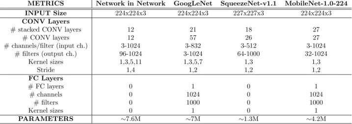
The complexity aspects of the selected DNN models are summarized in Table1, where the main features of the weighted layers are highlighted. Note that the entries ’# stacked CONV layers’ and ’# CONV layers’ for GoogLeNet and SqueezeNet do not match. This is simply due to the fact that the Inception and Fire modules of these models are composed of several parallel sub-layers.
The pre-trained weights of these models were downloaded from official repositories on GitHub supplied by each framework (see references in Table2). In the absence of a specific model on a particular framework, we translated it from Caffe since 1) this is the analyzed DL software that offers the largest set of pre-trained models; and 2) there are ready-made tools for conversion to Caffe221 and TensorFlow.36
METRICS Network in Network GoogLeNet SqueezeNet-v1.1 MobileNet-1.0-224
INPUT Size 224x224x3 224x224x3 227x227x3 224x224x3
CONV Layers
# stacked CONV layers 12 21 18 27
# CONV layers 12 57 26 27 # channels/filter (input ch.) 3-1024 3-832 3-512 3-1024 # filters (output ch.) 96-1024 3-1024 64-1000 32-1024 Kernel sizes 1,3,5,11 1,3,5,7 1,3 1,3 Stride 1,4 1,2 1,2 1,2 FC Layers # FC layers 0 1 0 1 # channels 0 1024 0 1024 # filters 0 1000 0 1000 Kernel sizes 0 1 0 1 PARAMETERS ∼7.6M ∼7M ∼1.3M ∼4.2M
Table 1: Main parameters defining the architectures of the DNN networks under study.
Network in Network GoogLeNet SqueezeNet-v1.1 MobileNet-1.0-224
Caffe [28] [29] [30] [31]
TensorFlow [28] [32] [30] [33]
OpenCV [28] [29] [30] [31]
Caffe2 [28] [34] [35] [31]
Table 2: Sources of downloaded pre-trained DNN models. Networks sharing the reference with Caffe correspond to models converted from the corresponding Caffe model as they were not available for that framework.
3. PERFORMANCE RESULTS
In this study, we used the Python binding for each of the introduced frameworks. The performance of the proposed DL components for real-time DNN inference on the RPi has been benchmarked through the following metrics:
1. Accuracy. We first checked the corresponding precision reported in the original research papers and
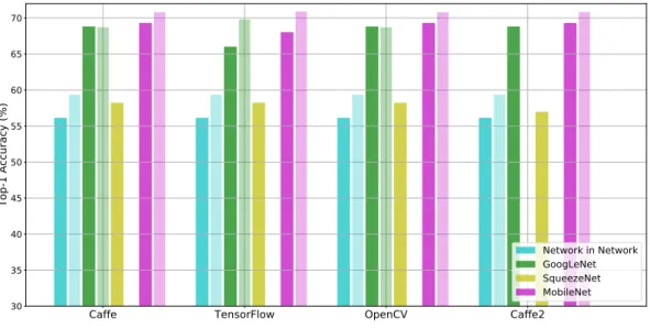
repositories. To this end, we calculated both Top-1 and Top-5 correct category classification rates over the 50k validation images of the ImageNet37 ILSVRC 2012 dataset. This dataset consists of variable-resolution color images encompassing 1000 object categories. Since the DNN models require fixed-size inputs, we resized the images to 256x256x3 and then cropped out the central patch with the desired resolution according to the DNN input size. We also subtracted the mean values over the dataset from each pixel. This pre-processing has been carried out with OpenCV functions and single-precision floating-point format. Mean substraction and scale values were extracted from the model repositories if provided, taking the mean value over the ImageNet dataset otherwise. It is worth noting though that accuracy figures were measured without any data augmentation, e.g. multiple crops, ensemble of multiple models etc. The results are shown in Fig.1. They mostly agree with the accuracy reported for the models. The small deviations could come from possible differences in the pre-processing carried out.
2. Throughput. We averaged the inference time over 100 images of the resized ImageNet set (256x256).
The only exception to this was for GoogLeNet with Caffe where the SoC of the RPi heats up significantly, forcing the CPU clock to go down. In this case, we computed the average fps rate over fewer images – around 64 – always ensuring that the CPU frequency was kept near its maximum, i.e. higher than 1100 MHz. The batch size was set to 1 since we are aiming at real-time video processing applications where latency should be minimal. Theframes per second rate has been calculated by summing the time required to get the input image ready for the particular model – i.e. the time required for scaling, mean subtraction etc. – and the inference time itself. Fig. 2 depicts the throughput achieved on each of the networks and frameworks under analysis.
Caffe TensorFlow OpenCV Caffe2 30 35 40 45 50 55 60 65 70 Top-1 Accuracy (%) Network in Network GoogLeNet SqueezeNet MobileNet
Caffe TensorFlow OpenCV Caffe2
55 60 65 70 75 80 85 90 Top-5 Accuracy (%) Network in Network GoogLeNet SqueezeNet MobileNet
Figure 1: Top-1 and Top-5 accuracies of the DNN models. Darker bars show measured values, while lighter ones stand for reported accuracies – if available, this is why there are missing lighter bars. The small deviations may be due to the application of slightly different image pre-processing.
3. Power Consumptionwhile performing inference. In order to reduce the impact of the operating system
on the performance, the booting process of the RPi does not start needless processes and services that could cause the processor to waste power and clock cycles in other tasks. We also disconnected all peripherals. Under these conditions, when idle, the system consumes around 1.3 watts. During the inference stage over the images, power consumption varies in a wide range of watts, as depicted in Fig. 3.
Caffe
TensorFlow
OpenCV
Caffe2
0 1 2 3 4 5Mean Throughput (fps)
2.1 0.8 3.1 1.1 2.6 1.7 4.2 2.4 1.4 1.3 4.8 2.6 2.5 0.9 3.7 1.8 Network in Network GoogLeNet SqueezeNet MobileNetFigure 2: Mean throughput (frames per second) for each considered model and framework.
Caffe
TensorFlow
OpenCV
Caffe2
1.5 2.0 2.5 3.0 3.5 4.0 4.5 5.0
Power
Consumption (W)
Network in Network GoogLeNet SqueezeNet MobileNetFigure 3: Power consumption limits and mean values.
meaningful way. It can be mathematically defined as:
FoM = Accuracy· Throughput
Power (1)
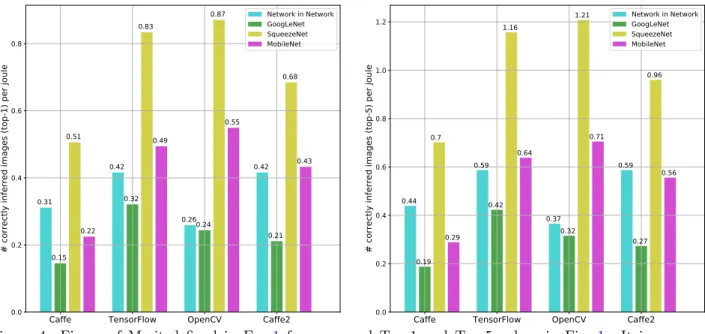
where ‘Accuracy’ features two flavors, namely Top-1 and Top-5. The results, shown in Fig.4, are presented in terms of ‘number of correctly inferred images per joule’, providing insight about the joint computational and energy efficiency of models and frameworks.
4. DISCUSSION
The first aspect to be stressed about the results just presented is that the performance of SqueezeNet is notably better than that of the other analyzed models, regardless of the considered framework. This network has the fewest parameters by far, leading to a smaller amount of required operations per inference and, therefore, to a higher throughput. The fact of being computationally lighter than the other models implies lower accuracy, but the FoM in Fig. 4 clearly indicates that SqueezeNet achieves the best balance. Conversely, GoogLeNet
Caffe TensorFlow OpenCV Caffe2 0.0 0.2 0.4 0.6 0.8
# correctly inferred images (top-1) per joule
0.31 0.15 0.51 0.22 0.42 0.32 0.83 0.49 0.260.24 0.87 0.55 0.42 0.21 0.68 0.43 Network in Network GoogLeNet SqueezeNet MobileNet
Caffe TensorFlow OpenCV Caffe2
0.0 0.2 0.4 0.6 0.8 1.0 1.2
# correctly inferred images (top-5) per joule
0.44 0.19 0.7 0.29 0.59 0.42 1.16 0.64 0.37 0.32 1.21 0.71 0.59 0.27 0.96 0.56 Network in Network GoogLeNet SqueezeNet MobileNet
Figure 4: Figure of Merit defined in Eq. 1 for measured Top-1 and Top-5 values in Fig. 1. It is expressed as ‘number of correctly inferred images per joule’ in order to emphasize the comparison between models and networks in terms of joint computational and energy efficiency.
performs the worst. Among the models in Table 1, this one is composed of the greatest number of weighted layers. The most recent model MobileNet, designed for mobile applications, is more accurate than SqueezeNet but also less efficient, according to the proposed FoM. There are MobileNet realizations not analyzed in this study (e.g., MobileNet-0.75-224, with∼2.6M parameters) that could likely get closer to the performance balance of SqueezeNet.
Among the evaluated software tools, both OpenCV and TensorFlow present the best performance in most of the models, while Caffe and Caffe2 yield similar results. This could be the consequence of better coding and exploitation of acceleration libraries. Furthermore, considering power consumption, OpenCV performs in a more steady way, featuring narrower intervals of power values. Comparing Caffe and Caffe2, the latter demands less power for all models, almost doubling the efficiency of the former for MobileNet.
These results broaden previous related research38on analyzing more frameworks, getting better performance in terms of throughput. Furthermore, the introduction of the aforementioned Figure of Merit enables a com-prehensive comparison between frameworks and models for the development of embedded vision applications. For specific scenarios where one of the benchmarked metrics is of special interest, variations of that FoM can be introduced, thus resulting in a more meaningful FoM according to prescribed specifications for the system.
In the near future, we will be adding more models and open-source software tools to the comparison. We will also extend our study to other low-cost embedded systems. Other considerations, such as the CPU temperature or the memory needed for more complex models, should also be considered.39
5. CONCLUSIONS
The presented benchmark is intended to serve as a preliminary reference when it comes to selecting DNN models and software frameworks among the broad ecosystem of DL components available these days. We have demonstrated that a cheap embedded computer like Raspberry Pi 3 Model B is capable of implementing real-time vision inference on the basis of complex DNN models categorizing among 1000 classes. OpenCV and SqueezeNet stand out as the best performing components according the proposed FoM. For a high prescribed throughput, OpenCV and TensorFlow are the best choices whereas for low energy budgets, OpenCV and Caffe2 are the most suitable tools. Finally, we have also shown that applications demanding both energy efficiency and high throughput must sacrifice accuracy by selecting simpler models or by tuning existing ones.
ACKNOWLEDGMENTS
The authors would like to thank Mr. Enrique Pardo for his help to set up benchmarking components. This work was supported by Spanish Government MINECO (European Region Development Fund, ERDF/FEDER) through Project TEC2015-66878-C3-1-R, and by Junta de Andaluc´ıa CEICE through Project TIC 2338-2013.
REFERENCES
[1] LeCun, Y., Bengio, Y., and Hinton, G., “Deep Learning,”Nature521(7553), 436–444 (2015).
[2] Verhelst, M. and Moons, B., “Embedded Deep Neural Network Processing,” IEEE Solid-State Circuits Magazine9(4), 55–65 (2017).
[3] Sze, V., “Designing Hardware for Machine Learning,” IEEE Solid-State Circuits Magazine 9(4), 46–54 (2017).
[4] Suleiman, A. et al., “Towards Closing the Energy Gap Between HOG and CNN Features for Embedded Vision,” in [Proc. IEEE International Symposium on Circuits and Systems], 444–447 (2017).
[5] Qualcomm, “Emerging Vision Technologies: Enabling a New Era of
In-telligent Devices.” 3 August 2016 https://www.qualcomm.com/documents/
emerging-vision-technologies-enabling-new-era-intelligent-devices. (Accessed: 22 Febru-ary 2018).
[6] Sze, V. et al., “Efficient Processing of Deep Neural Networks: A Tutorial and Survey,” Proceedings of the IEEE105(12), 2295–2329 (2017).
[7] “Raspberry Pi 3 Model B.” 2016https://www.raspberrypi.org/products/raspberry-pi-3-model-b/. (Accessed: 22 February 2018).
[8] “Raspbian.”https://www.raspberrypi.org/downloads/raspbian/. (Accessed: 22 February 2018). [9] Jia, Y. et al., “Caffe: Convolutional architecture for fast feature embedding,”arXiv(1408.5093) (2014). [10] “Caffe: a fast open framework for deep learning.”https://github.com/BVLC/caffe. (Accessed: 22
Febru-ary 2018).
[11] “Caffe. Model Zoo.”https://github.com/BVLC/caffe/wiki/Model-Zoo. (Accessed: 22 February 2018). [12] “OpenBLAS, optimized BLAS library based on GotoBLAS2 1.13 BSD version.” https://github.com/
xianyi/OpenBLAS. (Accessed: 22 February 2018).
[13] Abadi, M. et al., “Tensorflow: A system for large-scale machine learning,” in [12th USENIX Symposium on Operating Systems Design and Implementation (OSDI 16)], 265–283 (2016).
[14] “Deep Learning for Computer Vision with TensorFlow.” https://tensorflow.embedded-vision.com/. (Accessed: 22 February 2018).
[15] “A Docker image for Tensorflow.”https://github.com/DeftWork/rpi-tensorflow. (Accessed: 22 Febru-ary 2018).
[16] “TensorFlow-Slim image classification model library.” https://github.com/tensorflow/models/tree/ master/research/slim. (Accessed: 22 February 2018).
[17] “OpenCV.”https://opencv.org/. (Accessed: 22 February 2018).
[18] “Open Source Computer Vision Library.”https://github.com/opencv/opencv. (Accessed: 22 February 2018).
[19] “Caffe2.”https://caffe2.ai/. (Accessed: 22 February 2018).
[20] “Caffe2. Model Zoo.” https://github.com/caffe2/caffe2/wiki/Model-Zoo. (Accessed: 22 February 2018).
[21] “Caffe to Caffe2.” https://caffe2.ai/docs/caffe-migration.html#caffe-to-caffe2. (Accessed: 22 February 2018).
[22] Lin, M., Chen, Q., and Yan, S., “Network in network,”arXiv(1312.4400) (2013).
[23] Krizhevsky, A. et al., “Imagenet classification with deep convolutional neural networks,” in [Advances in Neural Information Processing Systems, NIPS], 1097–1105 (2012).
[24] Szegedy, C. et al., “Going deeper with convolutions,”arXiv(1409.4842) (2014).
[25] Szegedy, C., Ioffe, S., and Vanhoucke, V., “Inception-v4, inception-resnet and the impact of residual con-nections on learning,”arXiv(1602.07261) (2016).
[26] Iandola, F. et al., “Squeezenet: Alexnet-level accuracy with 50x fewer parameters and<1MB model size,” arXiv(1602.07360) (2016).
[27] Howard, A. et al., “Mobilenets: Efficient convolutional neural networks for mobile vision applications,” arXiv(1704.04861) (2017).
[28] “Model Zoo. Network in Network model.” https://github.com/BVLC/caffe/wiki/Model-Zoo# network-in-network-model. (Accessed: 22 February 2018).
[29] “BAIR/BVLC GoogLeNet Model.” 2017 https://github.com/BVLC/caffe/tree/master/models/bvlc_ googlenet. (Accessed: 22 February 2018).
[30] “SqueezeNet v1.1.” 2016https://github.com/DeepScale/SqueezeNet/tree/master/SqueezeNet_v1.1. (Accessed: 22 February 2018).
[31] “Caffe Implementation of Google’s MobileNets (v1 and v2).” 2018 https://github.com/shicai/ MobileNet-Caffe. (Accessed: 22 February 2018).
[32] “Inception V1.” 2016 http://download.tensorflow.org/models/inception_v1_2016_08_28.tar.gz. (Accessed: 22 February 2018).
[33] “MobileNet v1 1.0 224.” 2017 http://download.tensorflow.org/models/mobilenet_v1_1.0_224_ 2017_06_14.tar.gz. (Accessed: 22 February 2018).
[34] “Caffe2 Models. BVLC GoogLeNet.” https://github.com/caffe2/models/tree/master/bvlc_ googlenet. (Accessed: 22 February 2018).
[35] “Caffe2 Models. SqueezeNet.” https://github.com/caffe2/models/tree/master/squeezenet. (Ac-cessed: 22 February 2018).
[36] “Caffe to TensorFlow.” 2017https://github.com/ethereon/caffe-tensorflow. (Accessed: 22 February 2018).
[37] Russakovsky, O. et al., “ImageNet Large Scale Visual Recognition Challenge,” International Journal of Computer Vision (IJCV)115(3), 211–252 (2015).
[38] Pena, D., Forembski, A., Xu, X., and Moloney, D., “Benchmarking of CNNs for low-cost, low-power robotics applications,” (2017).
[39] “Raspberry Pi FAQs. Performance and Cost Considerations.”https://www.raspberrypi.org/help/faqs/ #topCost. (Accessed: 22 February 2018).