Occupancy Detection using Wireless Sensor Network in Indoor Environment

(1)

University of New Hampshire

University of New Hampshire Scholars' Repository

Master's Theses and Capstones Student Scholarship

Winter 2018

Occupancy Detection using Wireless Sensor

Network in Indoor Environment

Farah Ferdaus

University of New Hampshire, Durham

Follow this and additional works at:https://scholars.unh.edu/thesis

This Thesis is brought to you for free and open access by the Student Scholarship at University of New Hampshire Scholars' Repository. It has been accepted for inclusion in Master's Theses and Capstones by an authorized administrator of University of New Hampshire Scholars' Repository. For more information, please [email protected].

Recommended Citation

Ferdaus, Farah, "Occupancy Detection using Wireless Sensor Network in Indoor Environment" (2018).Master's Theses and Capstones. 1252.

(2)

Occupancy Detection using Wireless Sensor Network in Indoor Environment

By

Farah Ferdaus

Bachelor of Science in Electrical and Electronic Engineering, Bangladesh University of Engineering and Technology, 2015

Thesis

Submitted to the University of New Hampshire in Partial Fulfillment of

the Requirements for the Degree of

Master of Science in

Electrical Engineering

(3)

ii

This thesis has been examined and approved in partial fulfillment of the requirements for the degree of Master of Science in Electrical Engineering by:

Thesis Director, Nicholas J. Kirsch, Ph.D.

Associate Professor (Electrical and Computer Engineering)

John R. LaCourse, Ph.D.

Professor (Electrical and Computer Engineering)

Edward Song, Ph.D.

Assistant Professor (Electrical and Computer Engineering)

on 11/28/2018.

(4)

iii

DEDICATION

I would like to dedicate this thesis to my family. A special feeling of gratitude to my loving parents, my mother, Shahanara Begum, and my father, Abdullah Faruque for their encouragement and continuous support to achieve my dreams and goals. My beloved better half, B. M. S. Bahar Talukder, who is always inspiring and supporting me in my hard times and providing some great advice when I ran into problems, these are not only helpful but also lifesaving. My siblings, Shafayat Hossen, and Shuhail Hussain, who have always been there to cheer me up and stood by me through the good times and also in bad. They are my greatest sources of inspiration to go through tough times while keeping my head high.

(5)

iv

ACKNOWLEDGEMENT

I would like to thank Dr. Nicholas J. Kirsch for giving me the opportunity to work on this project and allowing me to work on something that I am truly passionate about. It is also my privilege to express my deepest and sincere appreciation to Dr. Kirsch for his direction and patience during the work associated with this thesis project. Dr. Kirsch was always available to answer questions despite an extremely demanding schedule. His guidance with thought-provoking objectives and support from the initial to the final level enabled me to develop a profound understanding and gain a wealth of engineering knowledge.

I would also like to express my deepest thanks to the members of my thesis committee, Dr. John R. LaCourse, and Dr. Edward Song for their willingness to serve on the committee. Their constructive and insightful comments helped me to improve my thesis.

I would also like to thank my fellow graduate students Jean Lambert Kubwimana, and Omid M. Kandelusy from the Wireless Systems Laboratory for assisting with the experimental setups. Last but not least, thank you to my family and friends who supported me throughout my education.

(6)

v

LIST OF TABLES

Table 2.1: Path loss exponents based on different environments[56] ... 13 Table 4.1: Simulation Parameters ... 57 Table 4.2: Combinations of sensors ... 62 Table 4.3: The probability of Correct Room Estimation in Kingsbury Measurement Campaign

with 4 sensors ... 68 Table 4.4: Simulation Parameters ... 73

(12)

xi

LIST OF FIGURES

Figure 1.1: This pie chart from the NHAPS study shows that Americans spend 86.9% of time

indoors, plus another 5.5% inside a vehicle[12] ... 2

Figure 1.2: Number of mobile phone users worldwide from 2015 to 2019 (in billions)[38] ... 5

Figure 2.1: The scenario ... 18

Figure 2.2: Simple Triangulation based on distance measurements between the receiver and transmitter ... 19

Figure 2.3: The comparison of area of overlap with and without shadowing ... 21

Figure 2.4: Position of sensors ... 24

Figure 3.1: System Schematic... 30

Figure 3.2: Intel NUC (Left) and Ettus VERT900 antenna connected with Ettus B200 (Right) . 31 Figure 3.3: Signal processing technique flowchart performed by each sensor ... 33

Figure 3.4: Fusion Server Schematic ... 35

Figure 3.5: Prerequisites required for building, installing, and running OpenBTS ... 36

Figure 3.6: OpenBTS system connections ... 38

Figure 3.7: Required steps for building, installing, and running OpenBTS ... 39

Figure 3.8: Antenna alignment ... 43

Figure 4.1: Map of Kingsbury Hall, South Wing, Second Floor, including sensors and measurement points ... 56

(13)

xii

Figure 4.2: Map of Kingsbury Hall, South Wing, Second Floor, including measurement points bounded by 6 sensors ... 59 Figure 4.3: The localization of MSE corresponding to distance for different positions of the unknown node from the origin with 6 sensors ... 60 Figure 4.4: Floor plan of Kingsbury Hall, Second Floor, including measurement points bounded by 4 sensors in two different combinations ... 64 Figure 4.5: Floor plan of Kingsbury Hall, Second Floor, including measurement points bounded by 4 sensors for ABDF combinations ... 65 Figure 4.6: The localization of MSE corresponding to distance for different positions of the unknown node from the origin with 4 sensors ... 66 Figure 4.7: Probability distribution of estimated error (MMSE) in Kingsbury Hall Measurement Campaign with 4 sensors (a) for A, B, D, F combination and (b) for B, C, D, F combination... 67 Figure 4.8: CDF of estimated error in Kingsbury Hall Measurement Campaign with 4 sensors . 69 Figure 4.9: MSE distribution in Kingsbury Hall Measurement Campaign with 4 sensors of an unknown node (a) the position of the sensors along with the actual and estimated position of the unknown node (b) only the actual and estimated position of the same unknown node ... 70 Figure 4.10: Map of SGH office ... 71 Figure 4.11: Partial Map of SGH office including sensors and measurement points ... 72 Figure 4.12: The localization of MSE corresponding to distance for different distances with 4 sensors ... 74

(14)

xiii

Figure 4.13: Probability distribution of estimated error (MMSE) in SGH office Measurement

Campaign with 4 sensors (ACDF combination) ... 75

Figure 4.14: The estimation error curve using MMSE, PML, EPML, and PMC[35] ... 76

Figure A.1: Screenshot of running rx_ascii_art_dft ... 102

(15)

xiv

LIST OF ACRONYMS

HVAC Heating, Ventilation and Air Conditioning

GPS Global Positioning System

WSN Wireless Sensor Networks

MMSE Minimum Mean Square Error

GSM Global System for Mobile Communications

NHAPS National Human Activity Pattern Survey

PIR Passive Infrared

CO2 Carbon Dioxide

CO Carbon Monoxide

TVOC Total Volatile Organic Compounds

RH Relative Humidity

RF Radio Frequency

RSS Received Signal Strength

PL Path Loss

(16)

xv SVM Support Vector Machine

SMP Smallest M-vertex Polygon

AoA Angle of Arrival

ToA Time of Arrival

TDoA Time Difference of Arrival

MLE Maximum Likelihood Estimation

PML Probability Based Maximum Likelihood

EPML Enhanced Probability Based Maximum Likelihood

MSE Mean Square Error

LS Least Square

SDR Software Defined Radio

USRP Universal Software Radio Peripheral

SIM Subscriber Identity Module

FFT Fast Fourier Transform

PSD Power Spectral Density

UHD USRP Hardware Driver

PSTN Public Switched Telephone Network

(17)

xvi GRC GNU Radio Companion

USB Universal Serial Bus

VID Vendor ID

PID Product ID

TDMA Time-Division Multiple Access

SIP Session Initiation Protocol

PBX Private Branch Exchange

ODBC Open Database Connectivity

ARFCN Absolute Radio Frequency Channel Number

PC/SC Personal Computer/Smart Card

USIM Universal Subscriber Identity Module

IMSI International Mobile Subscriber Identity

MCC Mobile Country Code

MNC Mobile Network Code

UL/DL Uplink/Downlink

RSSI Received Signal Strength Indicator

LUR Location Update Request

(18)

xvii IMEI International Mobile Equipment Identifier

MAC Media Access Control

MSISDN Mobile Station International Subscriber Directory Number

SMS Short Message Service

BTS Base Transceiver Station

SNR Signal-to-Noise Ratio

MS Mobile Station

SACCH Slow Associated Control Channel

BSC Base Station Controller

BCCH Broadcast Control Channel

CLI Command-Line Interface

NTP Network Time Protocol

HTTP Hypertext Transfer Protocol

RAM Random-Access Memory

CDF Cumulative Distribution Function

(19)

xviii

ABSTRACT

Occupancy Detection using Wireless Sensor Network in Indoor Environment

by

Farah Ferdaus

University of New Hampshire, December 2018

Occupancy detection plays an important role in many smart buildings such as reducing building energy usage by controlling heating, ventilation and air conditioning (HVAC) systems, monitoring systems and managing lighting systems, tracking people in hospitals for medical issues, advertising to people in malls, and to search and rescue missions. The global positioning system (GPS) is used most widely as a localization system but highly inaccurate for indoor applications. The indoor environment is difficult to handle because along with the loss of signals, privacy is a major concern. Indoor tracking has many aspects in common with sensor localization in Wireless Sensor Networks (WSN). The contribution of this work is the demonstration of a non-intrusive approach to detect an occupancy in a building using wireless sensor networks to detect energy from cell phones in a secure facility and perform indoor localization based on the minimum mean square error (MMSE). To estimate the occupancy, the detected cellular signals information such as signal amplitude, frequency, power and detection time is sent to a fusion server, matched

(20)

xix

the detected signals by time and channel information, performed localization to estimate a location, and finally estimated the occupancy of rooms in a building from the estimated locations.

(21)

CHAPTER 1

INTRODUCTION

The accurate occupancy detection of objects and people in indoor environments has long been considered an important building block for ubiquitous computing applications[1], [2]. In recent years, wireless devices are getting more powerful and pervasive. Current wireless devices often support more than one radio technology, e.g., WiFi, Bluetooth and the Global System for Mobile Communications (GSM). Most research on indoor localization systems has been based on the use of short-range signals, such as WiFi[3]–[5], Bluetooth[6], ultra sound[7], or infrared[8]. The wide availability of GSM networks encourages research on the use of GSM as a common radio technology. In addition, GSM signals appear more stable over time in comparison to WiFi or Bluetooth signals [9], [10]. In this thesis, we also opted for the use of GSM handset signaling. This chapter will present problems and the importance of occupancy detection, related previous work, this project’s contribution to science, and the organization of this thesis.

1.1

Motivation

Ubiquitous smartphone and location information enable new features of location-based services around local navigation, retail recommendation, proximity social networking, and location-aware advertising. Recently, the focus is also shifting geographically from outdoor to indoor. The indoor location market will be more enormous than outdoor since people spend more than 87% of the time indoor in the daily activities at the office, restaurant or home[11],[12]. Recent

(22)

2

studies show that the percentage of time spent in indoors is increasing nowadays. On average people spend 90% of their time indoors[13].

Figure 1.1: This pie chart from the NHAPS study shows that Americans spend 86.9% of time indoors, plus another 5.5% inside a vehicle[12]

Figure 1.1 shows broadly grouped statistics on the mean percentage of time that National Human Activity Pattern Survey (NHAPS) respondents spent in six different locations (residence, office-factory, bar-restaurant, some other indoor location, enclosed vehicle, and outdoors). Of the total time spent by all respondents on the diary day, 69% was spent, on average, in a residence (Figure 1.1). Approximately 87% of the time was spent indoors and 5-6% in a vehicle, with the remaining 7-8% spent outdoors. Time spent indoors (composed of time in a residence, in an office or factory, in a bar or restaurant, or in some other indoor location) and outdoors are represented by

(23)

3

different colored shaded slices. The percentages in the figure are the mean percentages taken over individual percentages for people in the NHAPS sample. Individual percentages were calculated from the time spent in each location over the total amount of time spent, which was equal to 24 h (1440 min) for each individual[12].

In dynamic environments, where the setting and occupancy keep changing, knowing occupancy information, including the number of the occupants and where they are located, can be beneficial in energy management. The other applications are public safety and services, security and emergency response such as search and rescue missions, asset tracking in hospitals etc.[14]. For example, congestion management in public places like malls, and tracking team members and assets on missions in the dark, or in crowded locations etc. Another example would be a section of the building that has more people will require more cooling or heating as compared to a section where a lesser number of people are present. Therefore, occupancy detection in an indoor environment is becoming increasingly important.

Building energy management and the necessity to reduce overall energy consumption is becoming an increasingly important topic. HVAC systems currently account for approximately half of the energy consumed in buildings in developed countries[15]. It is therefore essential to design and operate HVAC systems in an energy-efficient manner to meet low-energy targets. The HVAC need is strongly related to the occupancy of the building due to the air pollution and heat load generated by human metabolism, and their use of electrical equipment[16]–[19]. Conventional rule-based HVAC operation typically relies on a daily static occupancy schedule and real-time measurements of air temperature and/or CO2 concentration to determine the HVAC

need. However, several studies have suggested that significant energy savings can be achieved by using feedback from sensor-based occupancy detection when operating HVAC systems[20]–[29]

(24)

4

and lighting[30]–[32]. These studies demonstrate a significant theoretical energy-saving potential, i.e. when perfect occupancy detection and predictions are assumed. However, simulation results of Pedersen et al. [33] show that the accuracy of occupancy detection and predictions affects the theoretical energy-saving potential significantly. This calls for the development of reliable yet simple and inexpensive real-time occupancy detection approaches to include occupancy information when optimizing real-time HVAC operation.

Occupancy detection system in indoor environments (Indoor localization) is a technique for locating people or objects inside a building. Technologically, outdoor localization techniques cannot be directly moved to indoor[34]. GPS works almost perfectly in the outdoor environment but its accuracy, coverage, and quality deteriorate significantly in small-scale indoor places. Satellite-based GPS data can be difficult or impossible to access when a user is inside, or insufficient to accurately locate someone in a multistory building. This is a challenging problem for two reasons such as participant inclusion and access to trackable signals. The main challenge is the variability and multipath in the environment. Pre-deployed fixed infrastructure can be used to overcome the challenges. A few methods that use a pre-deployed infrastructure are as followed: Microsoft RADAR[3], RFID (Radio Frequency Identification) and the Vision-Based Approach[14]. This research is greatly inspired by the previous works[35]–[38] which is prototyped using OpenBTS, GNU Radio, and software-defined radios to verify the performance of indoor localization in the real-world environment.

(25)

5

1.2

Thesis Objective

Our goal is to develop an indoor occupancy detection scheme to make the system inexpensive with limited resources as well as environmentally friendly. Besides, the primary focus is to develop the detection technique that ensures accuracy and privacy. As the cell phone has become a ubiquitous device (Figure 1.2 shows the number of mobile phone users (in billions) worldwide from 2015 to 2019), therefore, detecting occupancy by tracing the location of the cell phone signal is a smart approach. To achieve this goal, the system requires the use of an RF (Radio Frequency) signal receiver to capture the GSM uplink frequencies.

(26)

6

The design of an occupancy detection service has several challenges that are related to the nature of the wireless medium and the GSM standards. These challenges are: how to capture GSM radio signals, and how to identify the channel information in order to provide the correct services? Facing these challenges requires an uplink receiver that captures, processes and analyzes GSM radio signals generated by the mobile devices. In this thesis, a wireless sensor network is used as a receiver for capturing GSM uplink signal frequencies. Moreover, our conducted measurements also revealed the insights on the GSM communication.

1.3

Related work

Current occupancy detection approaches can be divided into two groups: image-based methods and data-based methods. Image-based methods[40]–[43] rely on camera technology to detect occupancy. However, installing cameras can be perceived as a privacy violation and often represents an additional investment and running cost to a building project. Zhao et al.[44] obtained convincing occupancy detection in offices using a Bayesian belief network, which is a probabilistic graphical model (a type of statistical model) that represents a set of variables and their conditional dependencies via a directed acyclic graph, together with information from e.g. WiFi, GPS location, chair sensor, and keyboard and mouse sensor. However, some occupants may still consider these sensor data to be intrusive. Therefore, an inexpensive and non-intrusive alternative is required for indoor occupancy detection.

Currently, the most commonly used sensor data for occupancy detection is data from passive infrared (PIR) sensors[45]–[49] which are installed primarily for energy efficient operation of lighting. However, relying solely on PIR sensor data as a detection of occupancy is rather uncertain since the sensors do not capture immobile occupants or occupants that are outside the PIR sensor's

(27)

7

field-of-view[50]. Data from indoor climate sensors already used for conventional HVAC control seems like another basis for occupancy detection. The carbon dioxide (CO2) level in a room is an

attractive indicator as it is a direct consequence of human presence and, to some extent, independent of whether the occupants are moving or not[50]. The disadvantage of using the CO2

mass balance equation is that it requires detailed information about the physical room conditions (e.g. room volume, mechanical air change rate, window/door openings, occupant CO2 production,

outdoor CO2 concentration) which can be difficult to determine and vary in time, thus making it

subject to some uncertainty.

Utilizing sensor data to establish statistical models is another widely used approach[25], [49], [51]–[55]. Data-based occupancy detection based on measurements of CO2, carbon

monoxide (CO), total volatile organic compounds (TVOC), small particles (PM2.5), acoustics, illumination, PIR, temperature and relative humidity (RH) from an open-plan office environment was reported in[25], [49], [55]. The disadvantage of current methods for data-based occupancy detection is that they need prior information to work in practice. The above-mentioned methods based on physical models (mass balance equation) require detailed a priori information about the physical conditions of each room in the building. This type of method, therefore, needs to be set up manually before application. The above-mentioned statistical models need extensive training data and can therefore not be applied right after they are installed.

Thus, an alternative method to occupancy detection that overcomes the practical disadvantage of the model-based approaches is the novel plug-and-play method presented in this thesis to detect indoor occupancy. The proposed method was tested in long-time duration tests and evaluated in terms of its ability to detect occupancy compared to the ground truth.

(28)

8

1.4

Contribution

The contribution of this work is the implementation of an indoor occupant detection scheme by utilizing occupant-carried cellular devices. The proposed architecture is prototyped using OpenBTS, GNU Radio, and software-defined radios. All of the processing, such as detection of the energy of radio frequency from cell phones, transmission of the processed detected signal to a fusion server, performing localization algorithm over the processed data, is done in real-time. Therefore, significant energy savings can be achieved by operating HVAC controllers using a feedback from sensor-based occupancy detection methods. Furthermore, the proposed system model is applicable in any type of room shape and dimension and does not require the placement of the sensors in each room which potentially reduces cost. Finally, these sensors do not decode received cellular signals, so the privacy and identification of occupants are not of concern.

1.5

Thesis Organization

This section provides an explanation of each chapter of this thesis. This section helps the reader navigate this thesis and facilitates efficiency when particular sections are needed for review or reference.

Chapter 2 presents background information pertaining to this thesis project. Fundamental concepts required for understanding the occupant detection scheme using indoor localization and experimental results of this thesis project are explained.

Chapter 3 presents the hardware and software used to develop the prototype architecture and wireless sensor networks for occupancy detection. This chapter is important because it provides

(29)

9

specific information on how this project can be implemented. This chapter can also be referenced in order to facilitate other research projects that involve similar processes.

Chapter 4 presents empirical results and details the measurements made in Kingsbury Hall. It identifies the properties related to the proposed framework and the related assumptions. Tables and figures are provided in this chapter in order to organize results. The analytic information presented in this chapter proves this thesis is a contribution to science.

Chapter 5 concludes this thesis project, summarizing the results and the impact of the project. Also presents a focus for future work on this project. This chapter is important because it provides insight on what research needs to be conducted in order to increase the contribution of the systems presented in this thesis project.

(30)

10

CHAPTER 2

BACKGROUND INFORMATION

Path loss model, Received Signal Strength (RSS), sensor network and localization method are defined and conceptualized in this chapter. This information is presented in support of the experimental process and the results of this thesis project. The fundamentals of wireless communication are essential to this research. The first portion of this chapter explains basic propagation loss in wireless communications and signal propagation. Secondly, indoor localization is explained. Indoor localization is included to show how occupancy detection can be done by relative location estimation. Then, wireless sensor networks are explained so that the best number of sensors and the positioning of sensors for best results is understood. Finally, the Minimum Mean Squared Error (MMSE) is explained. The MMSE explains how this method works for localization problems. These processes are important because Chapter 3 uses these processes to design the wireless sensor network.

2.1

Propagation Loss

The mobile radio channel or environment places fundamental limitations on the performance of wireless communication systems. The transmission path between the transmitter and receiver can vary from a simple line of sight to one that is obstructed by buildings. These obstacles cause the wireless environment or channels to be random and unpredictable as well as complex. Movements by transmitter or receiver obstacles also may impact the signal levels.

(31)

11

There are five basic propagation mechanisms that mainly impact mobile communication by affecting the received power constructively or destructively[56]. These are reflection, diffraction, scattering, shadowing and path loss. These large-scale effects have an impact on the path loss between a transmitter and receiver.

Reflection occurs when an electromagnetic wave impinges upon an obstacle which has a large size in comparison to the wavelength of the propagating wave. Reflection may occur from any surface; from the surface of the earth and from buildings and walls.

Diffraction occurs when the electromagnetic wave is obstructed by a surface that has sharp edges or irregularities. The secondary waves resulting from the obstruction are present throughout the space and behind the obstacle. Diffraction gives rise to bending of waves around the obstacle, even though the line of sight might not exist between the transmitter and receiver. This phenomenon brings about a change in amplitude, phase, and polarization of the incident wave at the point of diffraction.

Scattering occurs when the environment through which the wave travels consists of objects which are smaller in dimension than the wavelength, and where the number of obstacles per unit volume is large. Scattered waves are produced by rough surfaces or irregularities in the channel.

Shadowing is the variation or the uncertainty in the environment. It is a zero mean Gaussian distributed random variable (in dBm) with standard deviation, 𝜎. Shadowing varies from building to building and even floor to floor inside a building.

Path loss (PL) or path attenuation is the difference in power or the loss in the signal strength due to the environment while traveling from the transmitter to the receiver. This loss of power is due to the radio wave propagation and objects in the environment (urban or rural, vegetation and

(32)

12

foliage), propagation medium (dry or moist air), the distance between the transmitter and the receiver, and the height and location of antennas. Theoretical and measurement based propagation models indicate that average received signal power decreases logarithmically with distance, in both the indoors and outdoors[56]. The PL does not take antenna gains or cable losses into consideration. PL is simply the attenuation present in the environment due to effects of free space propagation loss, reflection, refraction, scattering, shadowing, diffraction, aperture-medium coupling loss, and absorption. The PL is expressed as a function of the distance by using the path loss exponent, n. The value of n depends on frequency as well as the environment and also highly depends on the obstacles present in the path of the signal. In Equation (2.1), d0 is the reference distance, d is the distance between the transmitter and receiver, PL(d) is the path loss at distance d (in dBm) and n is the path-loss exponent which indicates the rate at which the path loss increases with distance, d0 is the far-field distance.

𝑃𝐿(𝑑) ∝ (𝑑 𝑑0

) 𝑛

(2.1)

Equation (2.1) can be written as follows where P(d) is the receiver signal strength at distance d (in dBm), P0(d0)is the received signal strength at distance d0 (in dBm).

𝑃(𝑑) = 𝑃0(𝑑0) − 10𝑛 log ( 𝑑 𝑑0

) (2.2)

In free space, n can be equal to 2 while in an environment with many obstacles, n will have a larger value. Table 2.1 lists the typical path loss exponents in various environments as mentioned in[56], [57].

(33)

13

Table 2.1: Path loss exponents based on different environments[57] ENVIRONMENT PATH LOSS EXPONENT, n

Free Space 2

Urban area cellular radio 2.7 - 3.5 Shadowed urban cellular radio 3 - 5

In-building line of sight 1.6 - 1.8 Obstructed in-building 4 - 6 Obstructed in factories 2 - 3

As in this thesis, indoor environments are dealt with, so the effect of materials generally present in indoors are needed to examine. Extensive surveys have been done on the probable value of the PL exponent in various buildings to find out the relation of n with power and increasing distance[34]. For example, signal levels greatly vary depending on whether doors are open or closed inside a building. Partitions are of two types: hard partitions and soft partitions. Hard partitions include parts of building structure like piping, walls, floors, windows etc. In contrast to hard partitions, soft partitions include partitions or materials that can be moved and do not span to the ceilings, like metallic devices, chairs, etc. The partition type also has a significant effect on n.

2.2

Indoor Localization Methods

The development of real-time locating systems has become an important add-on to many existing location-aware systems. While GPS has solved most of the outdoor locating problems, it fails to repeat this success indoors. A number of technologies have been used to address the indoor tracking problem. Indoor Localization is a system to locate objects or people inside a building using lights, radio waves, magnetic fields, acoustic signals, or other sensory information collected by mobile devices[58]. The research of localization has become a more and more important topic

(34)

14

with the popularity of ubiquitous mobile computing. In an indoor environment, many miniaturized wireless and sensing technologies have shown giant potential in positioning applications. The traditional indoor localization methods are:

 Fingerprinting  Dead-reckoning  Triangulation

2.2.1

Fingerprinting

Fingerprinting is a Radio Frequency based scene analysis. This method has two stages i.e. offline (training/survey) and online (query/run-time use)[59], [60]. Offline stage collects features known as fingerprints. Online stage estimates the location by matching online measurements against previously collected fingerprints. There are five common approaches to perform the analysis. These are Probabilistic, k Nearest Neighbor (kNN), Neural Networks, Support Vector Machine (SVM), and Smallest M-vertex Polygon (SMP)[61].

2.2.2

Dead-reckoning

Dead-reckoning is a device-centric and portable method less dependent on installed infrastructure. It starts with a known initial position, then estimates displacement and direction. Error accumulation is done over time and distance traveled. This method usually requires an accompanying alternative error control and reduction techniques[61].

(35)

15

2.2.3

Triangulation

Triangulation method is based on the geometric properties of triangles to determine location. It requires either range and/or direction information from/to reference points. The range-based case essentially uses the angle or distance information to estimate the location and distance measurements mostly through radio signals and ultrasound[3], [7], [62]. Both fingerprinting and dead-reckoning methods require an extra stage, offline stage, and alternative error control and reduction stage respectively, so to avoid the requirement of the additional stage in this thesis, the triangulation method was used. The next section describes more detail about the triangulation method.

2.3

Triangulation

The need for localization has brought forward a multitude of different approaches that vary depending on the type of information to be extracted from the signal and the environment. Based on signal metrics, the most popular and prevalent methods are[63], [64]:

 Angle of Arrival (AoA) (triangulation)  Time of Arrival (ToA) (trilateration)  Time Difference of Arrival (TDoA)  Received Signal Strength (RSS)

(36)

16

2.3.1

Angle of Arrival (AoA)

AoA determines the position of the user by measuring the angle at which the signal arrives at the receiver from the transmitter[34], [65]. Directional antennas have the capability to record the angle of arrival. However, this method is highly prone to multipath fading and requires a Line of Sight (LOS) with the receiver, which cannot be ensured in indoor environments. AoA is inconvenient because it involves geometric relationships that are used to locate the intersection of two lines.

2.3.2

Time of Arrival (ToA)

ToA measures the exact distance by using the travel time of the signal from the transmitter to the receiver. ToA systems are based on the precise measurements of the arrival time of a signal transmitted from a mobile device to several receiving sensors. Signals travel with a known velocity which is equal to the speed of light. ToA uses the equation Distance = Time x Speed to determine the location of Distance[34]. ToA requires precise knowledge of the transmission start time and must ensure that all receiving sensors are accurately synchronized with a precise time source. The amount of time required for a message from station X to arrive at receiving sensors A, B and C are recorded. Given a known velocity (the velocity of light), the distance can be calculated respectively. ToA is inconvenient and difficult because it involves absolute synchronization of the transmitter and the receiver which is often not possible.

2.3.3

Time Difference of Arrival (TDoA)

TDoA is similar to the ToA as both belong to the trilateration group which involves the intersection of the radii of the circles. ToA requires the synchronization of the transmitters and

(37)

17

receivers while TDoA requires the synchronization of the receivers. TDoA technique uses the relative measurements of time at each receiving sensor. The TDoA is calculated between the locations of sensors B and A as the positive constant k. The value of the TDoA between B and A can be used to construct a hyperbola with the foci at the receiving sensors A and B. The hyperbola represents all points on the x-y plane and the distance difference between the foci is k(c) meters. The unknown node lies along the hyperbola.

2.3.4

Received Signal Strength (RSS)

RSS is the relative signal strength at the receiver. The higher the RSS, the stronger the signal. Sensors or receivers deployed throughout an area of interest can sense the signal strength from a transmitter[66]. From this RSS[66], and signal path loss the distance between the unknown node and the sensor can be estimated. In this thesis, the RSS method has been used for localization.

A minimum of three sensors is always required for triangulation or trilateration with respect to RSS based methods. Popular localization methods include MLE (Maximum Likelihood Estimation), MMSE, PML (Probability Based Maximum Likelihood), and EPML (Enhanced PML).

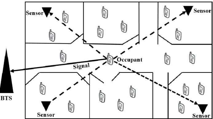
As an example of the system that is considered in this thesis, Figure 2.1 shows the considered scenario and the process of estimation of location. The cell phones are the position which is tried to estimate, and the triangles are the receivers or sensors. Now the question that arises is how an existing infrastructure can be used for indoor localization.

(38)

18

Figure 2.1: The scenario

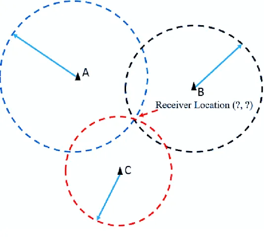
The main objective in localization is to use the received signal metrics, such as time and signal strength, to estimate the true distance between the receiver and each of the transmitters. The triangulation assumes the sensors to be the centers of circles and the distance between the receiver and transmitter to be the respective radii of the circle. The location is then estimated by determining the point at which all the circles intersect with each other as shown in Figure 2.2. In Figure 2.2 the transmitter positions are marked as A, B, C respectively. Thus, in the simplest form, the triangulation method needs at least three sensors. Once all the distances between the receiver and the transmitters are determined, the triangulation method can be used on them to determine the location of the unknown node (𝑥̂,𝑦̂). The location of the unknown node would then be the intersection of the circles.

(39)

19

Figure 2.2: Simple Triangulation based on distance measurements between the receiver and transmitter

This simple concept of triangulation has a very basic prerequisite that would only work if the distance measurements are perfect. In other words, all the circles have to coincide or intersect at a single unique point. The distance between the receiver and the transmitter can be determined by the distance equation. Let (X, Y) be the receiver location. Let (xi, yi) be the transmitter locations where i = 1, 2, 3...N and N is the total number of transmitters present. The distance between the receiver and each transmitter can be given by the Euclidean distance equation (2.3).

𝐷_𝑖 = √(𝑋 − 𝑥_𝑖)2_{+ (𝑌 − 𝑦}

(40)

20

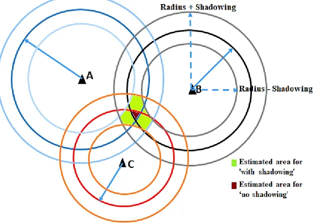
If there had been no shadowing and no variations in the environment, it would have been very easy to come up with a situation like Figure 2.2 where all the circles would have a common intersection point or a region of intersection such that the unknown point is inside the area of intersection. But in reality, wireless channels have multipath and shadowing. As a result, the region in which the unknown point might be present is larger. It is near impossible to determine or predict the area or region of overlap of the circles and thus it becomes very difficult to estimate the location of the unknown point in the indoor environment.

In Figure 2.3 the brown patched area corresponds to the region of overlap when there is no shadowing, while the green area corresponds to the region of overlap when shadowing is involved. Thus it can be easily said that shadowing increases the area of the region of overlap and makes localization a challenge. Essentially, a person’s location is tried to determine based on the signal strength received at the sensors marked as A, B, and C. By sensors, it is referred to antennas connected with software defined radios used to receive the signal strength from the unknown nodes (cell phones location).

(41)

21

Figure 2.3: The comparison of area of overlap with and without shadowing

2.4

Signal Metrics

The RSS method is based on the fact that the received signal decreases as the distance between the transmitter and receiver increases. Thus, by establishing a relationship or a rate at which the energy decreases, one can easily determine the distance between the transmitter and receiver with the knowledge of the received signal strength.

The log-distance path loss model, as shown in Equation (2.1) and Equation (2.2) indicates that the received signal strength decreases logarithmically with distance, in both outdoor and indoor environments. The relation between the path loss and the received signal strength can

(42)

22

simply be described as Pr = {Pt - PL} dBm, where Pr is the received signal power, and Pt is the transmitted signal power. The average received signal strength for an arbitrary separation between the transmitter and receiver, d can be expressed as a function of distance by using a path loss exponent, n[56].

Another inevitable and unavoidable environment variation factor is shadowing. In more precise terms, shadowing is the log-normal distribution that describes the randomness which occurs over a large number of measurement locations which have the same transmitter-receiver separation but have different levels of clutter on the propagation path. This is referred to as log-normal shadowing. Log-log-normal shadowing implies that measured signals have a Gaussian distribution about the distance-dependent mean where the measured signals have values in dBm units

It is possible to find a value of d based on knowledge of the other parameters. But a major problem with RSS is that the power attenuation with increasing distance is not monotonically decreasing. Issues like multipath and shadowing have an effect on the received signal strength. In environments that have various obstacles, there is more randomness which affects the calculation of d on the basis of received signal strength. As a result, Equation (2.2) changes to,

𝑃(𝑑) = 𝑃0(𝑑0) − 10𝑛 log ( 𝑑 𝑑0

) + 𝑋𝜎 (2.4)

Where,𝑋𝜎 is the zero mean Gaussian random variable with standard deviation, 𝜎 (dBm). When plotted on a log-log scale, the modeled path loss is a straight line with a slope equal to 10n dBm per decade.

(43)

23

2.5

Sensor Network

The number of sensors impacts the performance of the localization method[34]. In this section, the best number of sensors and the pattern in which the sensors should be set for best results are going to be discussed.

Localization methods either use all of the sensors to locate an unknown node or use a subset of sensors which yield the highest RSS. The basic logic behind the localization method is, if the received signal strength is higher, it would mean that the sensor is nearer to the unknown node in comparison to some other sensor, which results in lower RSS. Shadowing is log-normal in nature. The shadowing often results in a higher RSS for a farther sensor or vice versa[34]. That would result in the estimated point moving away from the actual point instead of estimating it better. As a result, it is required to find out the number of sensors that proves to be good for minimum errors in an indoor environment.

To understand the effect of the number of sensors on localization performance, different positions and numbers of sensors were considered for locating an unknown node. To fulfill the triangulation method, first, there had to be at least 3 sensors. Second, the sensors could not be in a line because that would not fulfill the triangulation condition. For the experiment, the sensors were always considered to be pre-deployed and their locations were already known.

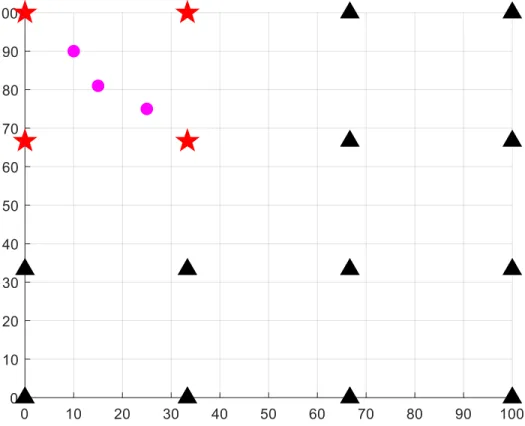
In [34]–[36] Ranita Bera et al. describe the method of deploying the sensors to result in a minimum error in indoor localization. There is a significant effect of a) using various numbers of sensors, b) the distance between the sensors and c) the area lying enclosed by the sensors. The test bed was a 100 X 100 meters region divided into a 4 X 4 grid. As a result, each grid width was 33.33 X 33.33 meters as shown in Figure 2.4. More sensors do not necessarily produce better

(44)

24

results rather the excess sensors actually move the estimated point from the actual location of the unknown point. Therefore, the positioning of sensors is more important than the number of sensors.

Figure 2.4: Position of sensors

Figure 2.4 shows the four sensors in a square formation that results in the least error in localization[35], [36]. The dots show the location of the unknown nodes. The red stars are the sensors being used for localization while the black triangles represent the remaining sensors that could have been chosen. The four sensors bounded the unknown nodes uniformly which resulted in a uniform low error in localization. Additionally, four sensors placed in a rectangular or square formation was a more feasible scenario than a triangular formation[34]. It is common understanding and knowledge that the centroid region, where the circles of content intersect, has

(45)

25

the least error. As a result, based on the literature review, it can be concluded that sensors bounding a rectangular or square region serves the best.

2.6

Minimum Mean Square Error (MMSE)

Mean Square Error (MSE) is a way of quantifying the difference between values implied by an estimator and the actual value of the quantity being estimated. Mean square error measures the average of the squares of the errors involved in the variables between the value implied by the estimator and the actual value that is being estimated. Suppose, let (x0,y0) be the coordinate of the unknown node and (𝑥̂, 𝑦̂) is the estimated coordinates of the unknown node in totally m times estimations. The MSE is as follows:

𝑀𝑆𝐸 = 1 𝑚 ∑(𝑥0− 𝑥̂0,𝑗) 2 𝑚 𝑗=1 + (𝑦0− 𝑦̂0,𝑗) 2 (2.5)

Now, minimizing the mean square error would mean that the error is minimum and the estimated point nearest to the actual point. This is known as the MMSE estimate.

In [67], Yung-Fa Huang et al. describe the method of MMSE based localization. The RSS at the receiver is attenuated with the distance in wireless communication channels. Moreover, the shadowing effect will ﬂuctuate the RSS with a log-normal distribution. Thus, the RSS at the receiver can be obtained by equation (2.6) where Pr(d) is the received power at an arbitrary distance, d and Pt is the transmitted power. Gt is the transmitter antenna gain and Gr is the receiver antenna gain. Again, 𝜆 is the wavelength; d is the distance between the transmitter and receiver and n is the path loss exponent[68]. The shadow fading, L is assumed to be the log-normal distribution model.

(46)

26

𝑃_𝑟(𝑑) = 𝑃𝑡𝐺𝑡𝐺𝑟𝜆

2

(4𝜋)2_𝑑𝑛_𝐿

(2.6)

After obtaining the power of RSS, Pr in the unknown node, the estimated distance can be calculated by the following equation (2.7). Where, the transmitter antenna gain, Gt and receiver antenna gain, Gr both is set to 1.

𝑑 = ( 𝜆 4𝜋) 2_⁄_𝑛 . (𝑃𝑡 𝑃_𝑟) 1_⁄_𝑛 _(2.7)

After the minimum three distance is obtained, the location of the unknown node is further estimated by the MMSE method[64], [69]. To construct the MMSE method for localization problems, the estimation error equation is formulated for the unknown node (x0,y0) by

𝑒_𝑛(𝑥₀, 𝑦₀) = 𝑑_𝑛− √(𝑥_𝑛− 𝑥₀)2_{+ (𝑦}

𝑛 − 𝑦0)2 (2.8)

Where x0 and y0 are the coordinates of the unknown node to be estimated, xn and yn are the known coordinates of the nth reference node, 𝑑_𝑛 is the estimated distance for the distance between the nth reference nodes and the unknown node. When the number of reference nodes is N, the index n would be 1, 2, ..., N. There are N simultaneous equations in (2.8).

To minimize the estimation errors, let 𝑒_𝑛(𝑥𝑛, 𝑦𝑛) = 0. Then through mathematical operations in (2.8), the (N-1) simultaneous equations are obtained by

𝑑_𝑛2 − 𝑥_𝑛2− 𝑦_𝑛2 − (𝑑_𝑁2 − 𝑥_𝑁2 − 𝑦_𝑁2) = 2(𝑥_𝑁− 𝑥_𝑛). 𝑥₀+ 2(𝑦_𝑁− 𝑦_𝑛). 𝑦₀ (2.9) By vector form, equation (2.9) can be rewritten as follows:

(47)

27 Where 𝑿 = [ 2(𝑥𝑁− 𝑥1) 2(𝑦𝑁− 𝑦1) ⋮ ⋮ 2(𝑥𝑁− 𝑥𝑛) 2(𝑦𝑁− 𝑦𝑛) ⋮ ⋮ 2(𝑥_𝑁− 𝑥_𝑁−1) 2(𝑦_𝑁− 𝑦_𝑁−1)] (2.11) 𝒘 = [ 𝑑₁2− 𝑥₁2− 𝑦₁2− (𝑑_𝑁2 − 𝑥_𝑁2 − 𝑦_𝑁2) ⋮ 𝑑𝑛2 − 𝑥𝑛2− 𝑦𝑛2− (𝑑𝑁2 − 𝑥𝑁2 − 𝑦𝑁2) ⋮ 𝑑_𝑁−12 − 𝑥_𝑁−12 − 𝑦_𝑁−12 − (𝑑_𝑁2 − 𝑥_𝑁2 − 𝑦_𝑁2)] (2.12) And 𝒃 = [_𝑦𝑥0 0] (2.13)

respectively. Using the Least Square (LS) method, the estimated coordinates of the unknown node is obtained by

𝒃̂ = [𝑥̂0

𝑦̂0] = (𝑿

𝑇_𝑿)−1_{. 𝑿}𝑇_𝒘 (2.14)

Thus the performance of localization can be investigated by mean square error mentioned in equation (2.5).

(48)

28

CHAPTER 3

PROTOTYPE ARCHITECTURE AND SENSOR NETWORK

The contribution of this work is to present an indoor occupancy detection technique using wireless sensor networks. The modeled infrastructure comprised of both hardware and software element enables the wireless sensor network system to detect the RF energy from cellular devices. This feature makes the system highly desirable for real-time applications.

In order to fully evaluate the performance capabilities of the sensor network in indoor occupancy detection, the framework was implemented using OpenBTS, GNU Radio, and software-defined radios. This chapter presents the software and hardware used in the execution of this thesis project.

The implementation process of the proposed prototyped architecture is very important to the outcome of this thesis project because the occupancy detection method is tested in a real-world application. Thus, in order to run the simulations, it is extremely important to build and install the system model precisely. The following chapter also covers each step of the software installation process to run the proposed system.

3.1

System Overview

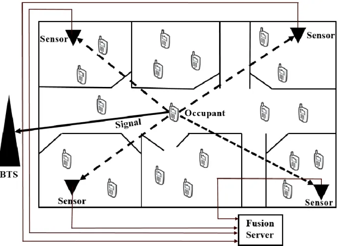
In this project, RF energy from occupants carried cellular devices to a base station is captured by sensors installed at known locations around a building. In our current framework, the receiver continuously scanned uplink channels of GSM band to check the presence of the signal from the

(49)

29

user. Each time a sensor detects a signal, information about the received power, time and channel of reception, and sensor number was sent to a fusion server. After the detection of RF energy, localization was performed using RSS and sensor information by the server. The server monitored the time and channel stamps of each entry from multiple sensors and matched entries with near-identical time and channel stamps. When three or more entries with near-near-identical time and channel stamps were matched then the information of those matched entries was fed into the localization algorithm, which estimates the occupant location. This collection occurs continuously, and as multiple occupant locations were collected and updated in the server, an estimate for room occupancy is made. Figure 3.1 illustrates how the cellular signals from occupants were captured by sensors around a building, then the sensors sent data to a fusion server, and the fusion server estimated occupancy from this information.

Ideally, the sensor must continuously detect and capture the RF energy of every nearby cellular device on every possible cellular channel. Sensors must be chosen or designed such that as many cellular channels can be monitored simultaneously as possible.

In the United States, cellular devices use the 700MHz, 750MHz, 800MHz, 850MHz, 1700MHz, 1900MHz, and 2100MHz bands. The bandwidth of each of these bands varies but is as high as 108MHz[38]. Each band is divided into multiple channels, each with a fixed bandwidth. Monitoring every band simultaneously with a single receiver would require an infeasible sampling rate with current technology. Realistically, multiple receivers monitoring each band, or a single receiver constantly sweeping over all bands are possible solutions. A single receiver constantly sweeping over all bands is a less expensive solution, however, this solution may miss the signal of a cellular device on one band while monitoring another, and therefore may underestimate occupancy. For our testbed, the search is restricted to a single band for proof-of-concept.

(50)

30

Figure 3.1: System Schematic

The remainder of this section includes details on hardware and software used in our testbed platform.

3.2

Hardware

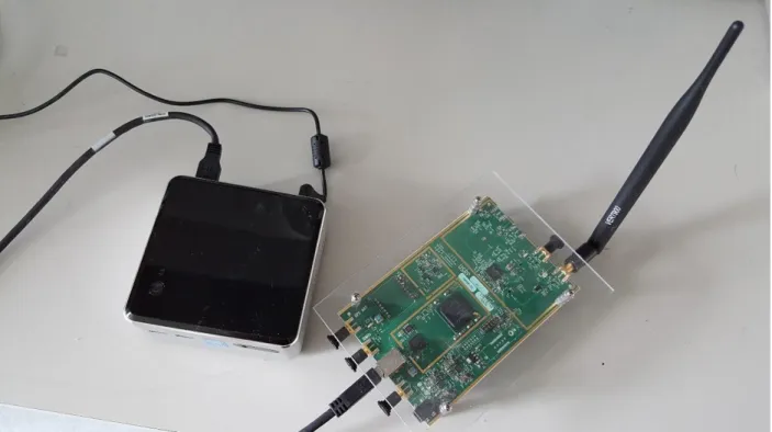
For this project, an Ettus Research USRP (Universal Software Radio Peripheral) B200 software defined radio board was chosen as a BTS as well as a receiver (sensor). This model has RF coverage from 70MHz to 6GHz, therefore covering all cellular bands. It can handle an instantaneous bandwidth of 56MHz, which is adequate for most cellular bands (but not all). It is powered over USB and transfers data to an associated compact and efficient host computer using

(51)

31

the USB 3.0 standard. This board also contains a Xilinx Spartan 6 XC6SLX75 FPGA, which can be programmed to perform signal processing on the received signal[70]. The USRP B200 is equipped with an Ettus VERT900 antenna, designed for use in 824-960MHz and 1710-1990MHz frequencies, thereby covering the majority of cellular (GSM) bands. A software defined radio (SDR) was chosen due to the ability to reprogram the device; a production system would be lower cost and designed specifically for this sensing application.

Figure 3.2: Intel NUC (Left) and Ettus VERT900 antenna connected with Ettus B200 (Right)

In addition to the receiver, the sensor must process the received signal, record the power, time and frequency of this signal, and send this information to a fusion server. While much of this will eventually be handled by an FPGA, a host computer connected to the USRP B200 currently handles the signal processing. The Intel NUC D54250WYKH was chosen for its small size, low power usage, processing power, and USB 3.0 capability. Figure 3.2 shows the VERT900 antenna

(52)

32

connected with USRP B200 paired with Intel NUC. This computer has a core i5 dual-core processor with turbo capability to achieve 2.6 GHz, 8GHz RAM, a 128GB SSD, and a WiFi adapter. The computer runs Ubuntu Linux, and controls the USRP B200 and processes the incoming signal using MATLAB. However, GNU radio can be a cheap alternative for such kind of application. The detected cellular signal power, time, and channel information were sent over an SSH/TCP/IP connection to the fusion server. From the server side, the collected data was analyzed using Python and stored in a database.

For testing purpose, our mobile network was modeled with the help of Open Source GSM Infrastructure (OpenBTS) implemented with a USRP B200 board which is equipped with two VERT900 antennas, one for transmitting GSM downlink frequencies and another for receiving GSM uplink frequencies, and customized Super SIM. OpenBTS is a C++ application that implements the GSM stack. The combination of OpenBTS and software-defined radios change the way of thinking about mobile networks and allowing the construction of complex radio networks purely in software.

3.3

Software

The important step in determining the location of the cell phones is the detection of the uplink signal transmitted to a base transceiver station (BTS) and process the detected signal accordingly to perform localization using RSS, the channel of reception, detection time and sensor information. For this project, MATLAB is used to process the detected signal and send the processed signal to the fusion server over a TCP connection.

(53)

33

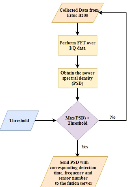
Figure 3.3: Signal processing technique flowchart performed by each sensor

In Figure 3.3 the main processing steps of RSS detection and extraction of detected information is illustrated. The whole processing is performed in MATLAB from the sensor side. Initially, the sampled I/Q data comes from USRP B200 board. Then Fast Fourier Transform (FFT) is performed over the sampled data, from which power spectral density (PSD) is calculated. After that, the maximum PSD is compared with a threshold, environmental noise level, to decide the

(54)

34

presence of RSS. Finally, the PSD and corresponding channel of reception, detection time and sensor information were sent to the fusion server over an SSH/TCP/IP connection.

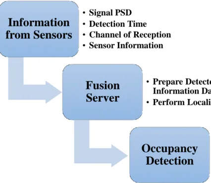
The fusion server was received the detected cellular signal information from each sensor. The data was received over a TCP/IP connection as a string, which is then parsed and stored in a database. Python is used to analyze the processed data and stored in a database for localization. In the server, the entries were matched with near-identical time and channel stamps by depending on the time and channel stamps of each entry. At least three entries with near-identical time and channel stamps are required to match, to feed the received power and sensor information into the MMSE based indoor localization algorithm. MATLAB is used to investigate the MSE performance of the localization. Thus a location estimation can be made. As each cellular device may communicate with a cellular BTS periodically, duplicate occupant entries may occur; this must be accounted for using a statistical model. Figure 3.4 illustrates the databases and functions of the server as a schematic.

(55)

35

Figure 3.4: Fusion Server Schematic

The following section demonstrates each step of the software installation process to run the proposed prototype architecture.

3.4

OpenBTS Installation

This section explains the building and installing of software and dependencies followed to develop the proposed framework. In order to efficiently rebuild this system, it is important that each mentioned version of the software is present during the installation process.

Several prerequisites are required before the system will be capable of building, installing, and running OpenBTS. Due to the compatibility issue, special care is required to select the appropriate version of the operating system (OS) and Open-source toolchain. USRP Hardware Driver (UHD) is fully supported on Linux, using the GNU Compiler Collection (GCC) and should work on most major Linux distributions.

Information

from Sensors

• Signal PSD • Detection Time • Channel of Reception • Sensor Information

Fusion

Server

• Prepare Detected Signal Information Database • Perform Localization

Occupancy

Detection

(56)

36

Although OpenBTS implements most of the complexity involved in building a mobile network in software, radio waves must still be transmitted and received somehow. Below are the hardware/software components required to procure implementing this capability in a development setting.

 Linux Desktop/Server  Software Defined Radio  Antennas

 Test Phones

 Test SIMs (Subscriber Identification Module )  Smart Card Writer

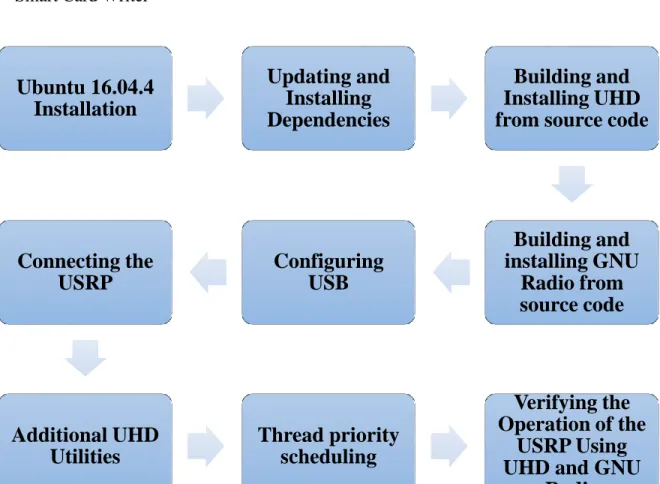
Figure 3.5: Prerequisites required for building, installing, and running OpenBTS

Ubuntu 16.04.4

Installation

Updating and

Installing

Dependencies

Building and

Installing UHD

from source code

Building and

installing GNU

Radio from

source code

Configuring

USB

Connecting the

USRP

Additional UHD

Utilities

Thread priority

scheduling

Verifying the

Operation of the

USRP Using

UHD and GNU

(57)

37

Figure 3.5 shows the steps required to follow to make the system prepare for building, installing, and running OpenBTS. Furthermore, Appendix A presents a step by step in detail procedure for installing the required prerequisite software and applications to develop the OpenBTS system. Ubuntu Desktop 16.04.4 LTS is required as the operating system. After installing the dependencies, the UHD and GNU radio should install from source code. Finally, it is required to verify the operation of USRP using UHD and GNU Radio. The following section describes the in detail installation process of OpenBTS.

3.4.1

Building, Installing and Running OpenBTS

The installation of a single instance of OpenBTS on a single computer with a single radio is described here. A complete installation of OpenBTS comprises the following components:

 OpenBTS itself: This is the GSM implementation from the Time Division Multiple Access (TDMA) part of Layer 1 up through Layer 3 and the Layer3/Layer 4 boundary.

 Transceiver: This is the software radio modem, implementing the lower part of Layer 1. OpenBTS starts the transceiver automatically.

 A SIP (Session Initiation Protocol) PBX (Private Branch Exchange) or softswitch (Asterisk): This component connects speech calls. This is not packaged with OpenBTS.

 Sipauthserver: This is the SIP registration and authorization server, used to process location updating requests from OpenBTS and perform corresponding updates in the subscriber registry database.

(58)

38

 Smqueue: This is the store-and-forward text messaging server. It needs to be started independently of OpenBTS. Smqueue is not required in installations that do not support text messaging.

In Figure 3.6 black links are the network connections (SIP), red links are the file system connections and the blue link is the Open Database Connectivity (ODBC) (network/local DB lookups) [71].

(59)

39

Figure 3.7: Required steps for building, installing, and running OpenBTS

Updating the

system and Git

Installation

Getting the

OpenBTS source

code

Selecting a

Branch or Tag

Installing

required

Libraries

Building the

OpenBTS Code

Installing

Packages

Installing

OpenBTS scripts

for systemd

Configuring

OpenBTS

Running

OpenBTS

Building and

Installing the

Subscriber

Registry and

Sipauthserve

Building and

Installing

Smqueue

Building and

Configuring

Asterisk

Running the

whole system

(60)

40

Figure 3.7 shows the steps required to follow for building, installing, and running OpenBTS. Furthermore, Appendix B presents a step by step in detail procedure for installing the software and applications to develop the OpenBTS system. Before installing the Git, the system needs to be updated. After that, the source code of OpenBTS is downloaded. Before building OpenBTS, the desired branch or tag for compilation ne