ISSN (print): 1978-1520, ISSN (online): 2460-7258
DOI: https://doi.org/10.22146/ijccs.50376 69
Classification of Traffic Vehicle Density Using Deep
Learning
Abdul Kholik*1, Agus Harjoko2, Wahyono3
1
Master Program in Computer Science, FMIPA UGM, Yogyakarta, Indonesia
2,3
Department of Computer Science and Electronics, FMIPA UGM, Yogyakarta, Indonesia e-mail: *[email protected], 2 [email protected], [email protected]
Abstrak
Tingkat kepadatan volume kendaraan merupakan suatu permasalahan yang sering terjadi di setiap kota, Adapun dampak dari tingkat kepadatan kendaraan adalah kemacetan. Pengelompokan atau klasifikasi tingkat kepadatan kendaraan pada jalan tertentu di perlukan karena setidaknya ada 7 kondisi tingkat kepadatan kendaraan. Pemantauan yang dilakukan oleh pihak kepolisian, Dinas perhubungan dan pihak penyelenggara jalan saat ini menggunakan berbasis video pengintai seperti CCTV yang masih dipantau oleh manusia/orang secara manual. Deep learning merupakan sebuah pendekatan mesin pembelajaran berbasis jaringan syaraf tiruan yang sedang giat dikembangkan dan diteliti akhir-akhir ini karena telah berhasil memberikan hasil yang baik dalam penyelesaian berbagai masalah softcomputing, Pada penelitian ini menggunakan arsitektur convolutional neural network. Penelitian ini dilakukan untuk mengotomasi klasifikasi pada tingkat kepadatan kendaraan dengan jumlah kategori adalah 7. Penelitian ini mencoba mengubah parameter pendukung pada convolutional neural network untuk menghassilkan akurasi maksimal. Setelah dilakukan percobaan mengubah parameter, model klasifikasi diuji menggunakan K-fold cross validation, confusion matrix dan penujian model dengan data testing. pada pengujian K-fold cross validation dengan hasil rata-rata 92,83% dengan nilai K(fold)=5, Pengujian model dilakukan dengan memasukan data testing berjumlah 100 data, model dapat memprediksi atau mengklasifikasi dengan benar yaitu 81 data.
Kata kunci—Kepadatan kendaraan, Deep learning, Klasifikasi, Convolutional neural network
Abstract
The volume density of vehicle is a problem that often occurs in every city, as for the impact of the vehicle density is congestion. Classification of vehicle density levels on certain roads is required because there are at least 7 vehicle density level conditions. Monitoring conducted by the police, the Department of Transportation and the organizers of the road currently using video-based surveillance such as CCTV that is still monitored by people manually. Deep Learning is an approach of synthetic neural network-based learning machines that are actively developed and researched lately because it has succeeded in delivering good results in solving various soft-computing problems, This research uses the convolutional neural network architecture. This research tries to change the supporting parameters on the convolutional neural network to further calibrate the maximum accuracy. After the experiment changed the parameters, the classification model was tested using K-fold cross-validation, confusion matrix and model exam with data testing. On the K-fold cross-validation test with an average yield of 92.83% with a value of K (fold) = 5, model testing is done by entering data testing amounting to 100 data, the model can predict or classify correctly i.e. 81 data.
Keywords—ComplexityVehicle density, Deep learning, Classification, Convolutional neural network.
1. INTRODUCTION
The level of vehicle density is an issue that often occurs in every city. The impact of vehicle density levels is congestion. Losses suffered from this congestion problem when the quantification in monetary unit is very large, i.e. losses due to travel time to be long and longer, vehicle operating costs become larger and vehicle pollution resulting in increasing.
Deep Learning introduces the Convolutional Neural Network (CNN) method which has excellent performance in pattern recognition and image classification. Convolutional Neural Network is designed to resemble human brain function, the computer will be given image data to learn, trained to recognize every visual element on imagery and understand its image pattern until later computer capable Identify the imagery. Convolutional Neural Network is an image recognition method that contributes greatly to the development of computer technology.
Deep learning implementation uses the Convolutional Neural Network (CNN) architecture on the fingerprint image classification using 80 fingerprint image data. The training process uses data that is 24 × 24 pixels and performs tests by comparing the number of epoch and learning rate so it is known that if the larger the number of epoch and the smaller the learning rate then the better the accuracy rate Training obtained. In this study, the level of training accuracy was achieved at 100% [1]. In the research that has been mentioned with very high accuracy results even reaching 100% of the authors see a deficiency IE occurs overfitting, therefore the author proposes a classification of the level of vehicle density using Deep learning specifically uses the Convolutional Neural Network architecture but to avoid overfitting that occurs in this research using cross-validation techniques and also dropout techniques.
2. METHODS
2.1 Traffic Behavior
The traffic behavior declares a quantity size that describes the conditions assessed by the road builder. Road traffic behaviors include capacity, travel time and average travel speed. Capacity is defined as the maximum current through a point on the path that can be maintained per hour unit under certain conditions. For two-way two-lane roads, capacity is determined for a bidirectional current (two-way combination), but for roads with multiple lanes, currents are separated per direction and capacity is determined per lane [2]. The basic equation for determining capacity is on the equation (1).
(1) Where:
= Capacity (SMP/hour)
= Basic Capacity (SMP/hourr) = Road width adjustment factor
= directional Separation adjustment factor (for undivided roads only) = adjustment factor of side barriers and road shoulders
= City size Adjustment factors
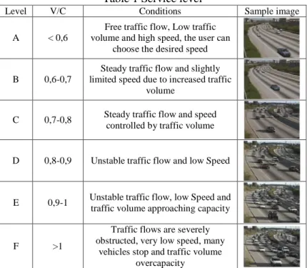
Service level is a measure of performance of roads or intersections calculated based on the level of road usage, speed, density, and obstacles occurring. Road service level calculations are based on comparisons of traffic volumes with road capacity known as the V/C ratio. The analysis of traffic density is based on road level calculation. The better the level of road service on a road, the lower the density of traffic.
Table 1 Service level
Level V/C Conditions Sample image
A < 0,6
Free traffic flow, Low traffic volume and high speed, the user can
choose the desired speed
B 0,6-0,7
Steady traffic flow and slightly limited speed due to increased traffic
volume
C 0,7-0,8 Steady traffic flow and speed
controlled by traffic volume
D 0,8-0,9 Unstable traffic flow and low Speed
E 0,9-1 Unstable traffic flow, low Speed and
traffic volume approaching capacity
F >1
Traffic flows are severely obstructed, very low speed, many
vehicles stop and traffic volume overcapacity
2. 1.1 CCTV
Closed Circuit Television (CCTV) according to a recording tool that uses one or more video cameras and generates video or audio data. CCTV has the benefit of being able to record all activities remotely without any distance limitation, can monitor and record all forms of activities that occur on the observation site using a laptop or PC in real-time from anywhere, and can be Recording the entire incident by 24 hours, or can record when a movement of the monitored area occurs [3].
2. 1.2 Image
An image or image is a spatial representation of an actual object in the two-dimensional field usually written in X-y Cartesian coordinates, and each coordinate represents one smallest signal of the object [4]. A digital image is a two-dimensional function, f (x, y), which is a function of light intensity where the x and Y values are spatial coordinates and function values at each point, and (x, y) is the level of imagery in that point. A digital image is indicated by a matrix in which the row and its column state a point on the image and its matrices (referred to as the image or pixel element) state the level of the grey at that point. The matrix of digital imagery is N x M (Line × column), with:
N = number of line 0 ≤ y ≤ N – 1
M = number of columns 0 ≤ x ≤ M – 1
L = highest value for the degree of grey 0 ≤ f(x,y) ≤ L – 1 The values of the grey degrees can be expressed in a matrix-like equation (2).
(2)
2. 2 Image Preprocesing
Image preprocessing is done to prepare a better image for feature extraction needs or classification needs. Image preprocessing has several commonly used techniques such as eliminating noise with Gaussian blur, segmentation and resizing.
2. 2.1 RGB Color Conversion to Grayscale
Changing the image color to grayscale from red, green, and blue or RGB makes it easier to process digital imagery. The method of converting an image from RGB to Greyscale is the Average value method and the Luminance value on the image. The Average method is the simplest method of changing the image color space from RGB to greyscale. The average method can be done using equations (3) [5].
(3)
2. 2.2 Cropping
Cropping is a way of making certain areas of interest in imagery, which aims to make it easier to analyze imagery and reduce the size of imagery irregularities. In the image processing process, usually not the overall scene of the image we use, to get the area we want we can cut the image [6]. Image Cropping can be used for spatial data as well as spectral data. Image cropping can be done based on the coordinate point, the number of pixels or zooming results of certain areas.
2. 3 Deep Learning
Deep Learning is one of the techniques in machine learning that utilizes many non-linear information processing layers to perform feature extraction, pattern recognition, and classification. Deep learning is a problem-solving approach to computer learning systems that use a hierarchical concept. The concept of hierarchy makes computers able to learn complex concepts by combining them from simpler concepts. If it is depicted as a graph of how the concept is built on another concept, this graph will be in with many layers, it is the reason it is referred to as deep learning [7].
2. 3.1 Convolutional Neural Network
The Convolutional Neural Network (CNN) is one of the algorithms of deep learning which is the development of Multilayer Perceptron (MLP) designed to process data in two-dimensional forms, such as images or sound. CNN is used to classify data labeled using a supervised learning method or well-curated learning. CNN is often used to recognize objects or landscapes and performs object detection and segmentation. CNN learns directly from its image data thereby eliminating feature extraction manually [8]. The overview of CNN architecture can be shown in Figure 1.
Figure 1 architecture convolutional neural network
Figure 1 shows the architecture of CNN that consists of several stages of operation. The operating stages are convolution operations, pooling operations and activation functions.
2. 3.2 Convolution Operation
Basic operations in CNN is convolution operation or h(x). Convolution has two functions f(x) that are functions of the original object and g(x) as a convolution kernel function that is defined as an equation (4).
The convolution operation is also imposed on the S(t) function of a multi-dimensional array value can be formulated like the equation (5).
(5) Where:
S (t) = function of the convolution operation results x = multi-dimensional array containing data w = weight or commonly referred to as filter t = variable of function
A = dummy variable constants
In machine learning applications, weights (w) are multi-dimensional arrays which are parameters that can be learned.
2. 3.2 Activation Function
The activation function is calculated after convolution operation. Activation functions that are often used in convolutional neural networks include tanh(), ReLu (Reactified Linear Unit), sigmoid, and softmax [8]. This research will be use ReLu and SoftMax activation functions.
1. The ReLu function is a function that the output value of a neuron can be expressed by 0 if the input value is negative. If the input value is positive, then the output of the neuron is the input value of the activation itself. The equation of this function can be shown in equations (6).
(6)
2. Softmax activation is applied in the last layer of the neural network. Softmax is more commonly used than the ReLU activation function, sigmoid or tanh (). Softmax is useful for converting the output of the last layer in neural networks to basic distribution probability. The Softmax equation is shown in the equation (7).
(7)
2. 3.3 Pooling Operation
After calculating activation function, pooling operations are carried out by reducing size of matrix by means of max-pooling or average-pooling. Output from pooling operation is a matrix with smaller dimensions compared to the initial image. Convolution and pooling process is carried out to obtain the desired feature map to be input into fully connected layer [8]. The pooling illustration is shown in Figure 2, namely pooling by max-pooling.
Figure 2 Pooling with max-pooling
2. 3.4 Pooling Operation
Stride Stride is a parameter that determines number of filter shifts in an image pixel. If the stride value is 1, the convolution filter will shift by 1 pixel horizontally and vertically. More
smaller stride value, model will capture more detailed information from an input image, but it requires more computation when compared to a large stride [8]. A small stride value does not always produce better pixel information details, but with a small stride value prevents stacking of unused pixel information.
2. 3.5 Padding
Padding Padding or Zero Padding is a parameter that determines number of pixels (containing a value of 0) to be added to each side of the input. This is used in order to manipulate the output dimensions of the convolution layer (Feature Map) [9]. Purpose using padding layer is output dimensions of the convolution layer will always be smaller than the input (except the use of a 1x1 filter with stride 1) so that more information is wasted which is not needed when the convolution process is running. In addition, zero padding will set output layer's dimensions to remain the same as the input dimension or at least not drastically reduced. If in a dimension actually input is 5x5, then convolution is done with a 3x3 and stride filter of 2, then a 2x2 feature map will be obtained. But if you add zero padding with a value of 1x1, then the resulting map feature is 3x3 (more information is generated). Calculating the dimensions of a feature map can be used the following equation (8).
(8)
Where: V = Volume Size F = Filter height P = Zero Padding S = Stride 2. 3.6 Adam OptimizerAdam's optimization was introduced by Diederik Kingma from OpenAI and Jimmy Ba from the University of Toronto in 2015 ICLR paper entitled "Adam: A Method for Stochastic Optimization". Adam stands for Adaptive Moment Estimation [10]. Adam optimizer is an optimization algorithm that is used as a substitute for classic gradient stochastic procedures that will update network weights based on iteratives without changing the learnign rate. The algorithm from Adam Optimizer is shown in Figure 3.
Figure 3 Adam optimizer algorithm
3. RESULTS AND DISCUSSION
3. 1 Data and Pre-processing
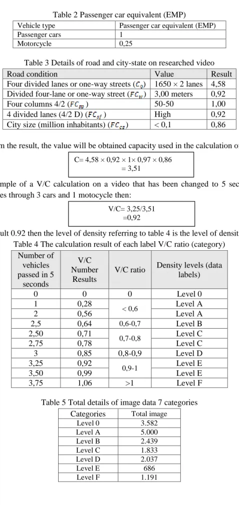
This research uses CCTV video data taken via DISHUB Sukoharjo, the existing video data will be converted into image data. In this research video data is changed to 5 seconds per video. Authors add one category to make it easier on classification Peros. How to assign categories or labels to individual data using the V/C ratio.
Table 2 Passenger car equivalent (EMP)
Vehicle type Passenger car equivalent (EMP) Passenger cars 1
Motorcycle 0,25
Table 3 Details of road and city-state on researched video
Road condition Value Result
Four divided lanes or one-way streets ( ) 1650 × 2 lanes 4,58 Divided four-lane or one-way street ( ) 3,00 meters 0,92
Four columns 4/2 ( ) 50-50 1,00
4 divided lanes (4/2 D) ( ) High 0,92
City size (million inhabitants) ( ) < 0,1 0,86
From the result, the value will be obtained capacity used in the calculation of V/C.
Example of a V/C calculation on a video that has been changed to 5 seconds, if the vehicle passes through 3 cars and 1 motocycle then:
With the result 0.92 then the level of density referring to table 4 is the level of density E. Table 4 The calculation result of each label V/C ratio (category)
Number of vehicles passed in 5 seconds V/C Number Results
V/C ratio Density levels (data labels) 0 0 0 Level 0 1 0,28 < 0,6 Level A 2 0,56 Level A 2,5 0,64 0,6-0,7 Level B 2,50 0,71 0,7-0,8 Level C 2,75 0,78 Level C 3 0,85 0,8-0,9 Level D 3,25 0,92 0,9-1 Level E 3,50 0,99 Level E 3,75 1,06 >1 Level F
Table 5 Total details of image data 7 categories Categories Total image
Level 0 3.582 Level A 5.000 Level B 2.439 Level C 1.833 Level D 2.037 Level E 686 Level F 1.191 V/C= 3,25/3,51 =0,92 C= 4,58 × 0,92 × 1× 0,97 × 0,86 = 3,51
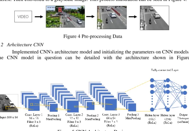
3. 2 Pre-processing Data
Data pre-processing is done to produce better, more computable data. CCTV video is transformed into image on every frame in the video. Images are cut according to the region of interest. Then converted to a grayscale image. This process illustration can be seen in Figure 4.
Figure 4 Pre-processing Data
3. 2 Arhcitecture CNN
Implemented CNN's architecture model and initializing the parameters on CNN models. The CNN model in question can be detailed with the architecture shown in Figure 5.
Figure 5 CNN Architecture Design
3. 3 Parameter effect on CNN
The implementation of CNN's model with a good value of accuracy should be
accompanied by parameters that help to produce the best accuracy value. The
parameters in question are the many convolution layers, the number or size of the filter
of each layer, the number of neurons in the hidden layer, and the learning rate.
3. 3.1 Effect of Epoch number
Epoch is when the entire dataset is already going through the training process on
the Neural Network until it is returned to the beginning for one round. In this
experiment, the number of epoch given is in table 6.
With almost the same accuracy results between epoch 50 and 60 but this study considers the time when training is fewer then the best epoch selection is 50 epoch.Table 6 Effect of Epoch number Epoch Training Accuracy
10 78.82% 20 81.19% 30 82.55% 40 83.68% 50 84.48% 60 84.57% 70 84.11% 80 78.82%
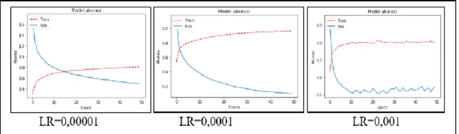
3. 3.2 Effect of Learning rate
The value of learning rate is done to produce a model with a steady and minimal training loss value. The value of the learning rate is given when the CNN model is ready to compile using Adam optimizer. The value of the learning rate provided is 0.0001, 0.001, and 0.001.
Figure 6 Effect of learning rate
Learning rate 0.001 almost experienced a stable similarity with the value of leraning rate 0.00001 But the result of loss greater than 54.39%. With this experiment, this research uses the value of learning rate that produces the best accuracy with learning rate 0.0001.
3. 3.3 Effect without or using Dropout
Dropout is one of the efforts to prevent the occurrence of overfitting and also accelerate the learning process. Overfitting is a condition where almost all data that has been through the training process reaches a good percentage, but there is a discrepancy in the predictive process. In its working system, Dropout eliminates while a neuron is a hidden layer or a visible layer located inside the network. Results effect using or without dropout to show the best accuracy when using a dropout of 0.1 with an accuracy of 92.73%. Results effect using or without dropout experiments demonstrated by table 7.
Table 7 Pengaruh dropout
Dropout Training loss Training Accuracy
- 33,34% 87,32% 0,1 17,91% 92,73% 0,2 25,61% 89,91% 0,25 26,91% 89,42% 0,3 33,50% 86,79% 0,50 54,86% 78,43% 0,7 76,76% 70,49%
3. 3.4 Effect Filter Size
A certain sized convolution (filter) kernel, the computer gets new representative information from the multiplication of parts of the image with the filter used. From the effect of filter size, the best filter size is obtained at 4 × 4 sizes. The bigger the filter size is used, the better the accuracy is 94.67%.
Table 8 Effect Filter Size
Filter size Training loss Training_accuracy
2×2 17,91% 92,73%
3×3 14,69% 94,26%
3. 3.5 Effect Pooling
The best max-pooling size is 2 × 2 which generates 94.26% accuracy, but taking into consideration the results of his training loss then the one used for this research is max pooling with size 3 × 3.
Table 9 Effect pooling
Max pooling size Training loss Training accuracy
2×2 17,91% 92,73%
3×3 14,69% 94,26%
4×4 38,19% 85,73%
3. 4 Effect of Edge Image Data Input
The result of the accuracy of the training on the edge image is aimed at table , the grayscale and edge image example can be seen in image 1. Better result in the show on the edge image of grayscale image due to the absence of blur or difference in light levels Images that affect the value of existing pixels. The accuracy of the data training on this edge image is 95.82%.
Figure 7 sample data input image
Table 10 Results of the effect edge image data input Image data input Training loss Training accuracy
Grayscale 13,80% 94,64%
Edge 11,09% 95,82%
3. 5 Evaluation using Confusion Matrix
This evaluation aims to test the performance of the classification model that has been created by the system. With data validation amount of 3364 data. Precision, recall and F1-score results can be viewed in table.
Table 11 Precision, recall and F1-score results Level precision recall f1-score support
0 0.92 0.95 0.94 718 A 0.96 0.88 0.91 1000 B 0.52 0.75 0.62 491 C 0.91 0.29 0.44 369 D 0.31 0.37 0.34 409 E 0.15 0.09 0.11 138 F 0.38 0.5 0.43 239
Result of validation confusion matrix with validation data amounting to 3364. Visible density level A obtains A true 683 value of 718 image data or if normalized 92%. The occurrence of minimal results from the evaluation of confusion matrix at the level of this E because of the image data in the low training, resulting in poor predictions also.
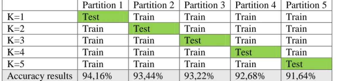
3. 5 Evaluation using K-fold Cross Validation
This study will try testing using stratified K-fold cross-validation with value K = 5. Each partition gets the result of each training accuracy. The accuracy results are calculated and the average search is 92.83%. With the average result not far from the results of the accusation of each partition can be concluded if the distribution of dataset training and also testing is correct with the greatest accuracy gained on partition 1.
Table 12 K-fold Cross Validation results
Partition 1 Partition 2 Partition 3 Partition 4 Partition 5
K=1 Test Train Train Train Train
K=2 Train Test Train Train Train
K=3 Train Train Test Train Train
K=4 Train Train Train Test Train
K=5 Train Train Train Train Test
Accuracy results 94,16% 93,44% 93,22% 92,68% 91,64%
3. 6 Evaluation CNN model with Testing data
Test experiments use data as much as 50 and 100 that the category spread is balanced. Test results with grayscale images tend to be smaller than the edge image. From the results of data testing the input grayscale image amounted to 50 CNN models were only able to categorize correctly 29 only while from the trial of the 100 edge model image CNN could properly predict 81 data.
Table 13 Model test results with data testing Amount of data Correct predictions Wrong predictions
Grayscale 50 29 21
100 45 65
Edge 50 36 14
100 81 19
4. CONCLUSIONS
The effect of using edge image input data shows better results compared with grayscale image input, with 94.64% accuracy for grayscale image and 95.82% for the edge image. In this study, the use of the learning rate parameter with a value of 0.0001 can be a suitable parameter that results in the least small training loss.
The use of dropout in this study with a value of 0.1 resulted in better training accuracy of 92.73% compared to not using dropout ie 87.32%. Using an edge input image of testing 100 data testing processed through the CNN model created. Models can classify into density-level categories correctly amounting to 81 data.
ACKNOWLEDGEMENTS
REFERENCES
[1]
Nurfita, R. D. and Ariyanto G., “Implementasi Deep Learning Berbasis
Tensorflow Untuk Pengenalan Sidik Jari”
Emitor: Jurnal Teknik Elektro,
18,
22-27. 2018.
[2]
Bina Marga Direktoral Jendral, “
Manual Kapasitas Jalan Indonesia
(MKJI)”,
Jakarta, 1997.
[3]
Surjono, H., “Eksperimen Pengiriman sinyal televisi dengan pemancar TV dan
CCTV serta Pemanfataanya dalam Pendidikan”,
Journal PTK,
07, 37-43, 1996.
[4]
Gonzalez, R.C. dan Woods, R.E., “
Digital Image Processing 3rd ed”
, Prentice
Hall, 2008.
[5]
Kanan, C. and Cottrell, G.W.,
“Color-to-grayscale: Does the method matter in
image recognition”
, PLoS ONE, 7(1), 2012.
[6]
Arhatin, R., E., “
Memotong Citra, Koreksi Radiometrik dan Koreksi Geometrik”,
2010.
[7]
Goodfellow, I., Bengio, Y., dan Courville, A., “
Deep Learning”
, MIT Press,
USA, 2016.
[8] Dzulqarnain M. F., Suprapto., Makhrus, F., Improvement of Convolutional Neural Network Accuracy on Salak Classification Based Quality on Digital Image”, IJCCS (Indonesian Journal of Computing and Cybernetics Systems), Vol.13, No.2, April 2019, pp. 189~198, 2019. [Available:
https://jurnal.ugm.ac.id/ijccs/article/view/42036.
[Accessed: 03-October-2019]
[9] Y. Pang, M. Sun, X. Jiang, and X. Li, “Convolution in Convolution for Network in Network,” IEEE Transactions on Neural Networks and Learning Systems, vol.29, no. 5, 2018. Available:
https://ieeexplore.ieee.org/document/7879808
. [Accessed: 03-October-2019][10] Kingma D. P., and Ba J., “Adam: A Method for Stochastic Optimization,” Cornell University Library, Jan. 2017. Available: