Adaptive mesh refinement in topology optimization

(1)

c

(2)

ADAPTIVE MESH REFINEMENT IN TOPOLOGY OPTIMIZATION

BY

MIGUEL A. SALAZAR DE TROYA

DISSERTATION

Submitted in partial fulfillment of the requirements

for the degree of Doctor of Philosophy in Mechanical Engineering

in the Graduate College of the

University of Illinois at Urbana-Champaign, 2019

Urbana, Illinois

Doctoral Committee:

Professor Daniel A. Tortorelli, Chair and Director of Research

Professor Phillipe Geubelle

Professor Arif Masud

(3)

Abstract

This dissertation presents developments in stress constrained topology optimization with Adaptive Mesh Refinement (AMR).

Regions with stress concentrations dominate the optimized design. As such, we first present an approach to obtain designs with accurately computed stress fields within the context of topology optimization. To achieve this goal, we invoke threshold and AMR operations during the optimization. We do so in an optimal fashion, by applying AMR techniques that use error indicators to refine and coarsen the mesh as needed. In this way, we obtain accurate simulations and greater resolution of the design domain in a computationally efficient manner. We present results in two dimensions to demonstrate the efficacy of our method.

The topology optimization community has regularly employed optimization algorithms from the opera-tions research community. However, these algorithms are implemented in the Euclidean space instead of the proper function space where the design, i.e. volume fraction, field resides. In this thesis, we show that, when discretizing the volume fraction field over a non-uniform mesh, algorithms in Euclidean space are mesh de-pendent. We do so by first explaining the functional analysis tools necessary to understand why convergence is affected by the mesh. Namely, the distinction between derivative and gradient definitions and the role of the mesh dependent inner product. These tools are subsequently used to make the Globally Convergent Method of Moving Asymptotes (GCMMA), a popular optimization algorithm in the topology optimization community, mesh independent. We then benchmark our algorithm with three common problems in topology optimization.

High resolution three-dimensional design models optimized for arbitrary cost and constraint functions are absolutely necessary ingredients for the solution of real–world engineering design problems. However, such requirements are non trivial to implement. In this thesis, we address this dilemma by developing a large scale topology optimization framework with AMR. We discuss the need for efficient parallelizable regularization methods that work across different mesh resolutions, iterative solvers and data structures. Furthermore, the optimization algorithm needs to be implemented with the same data structure that is used for the design field. To demonstrate the versatility of our framework, we optimize the designs of a three dimensional stress

(4)

(5)

(6)

Acknowledgments

I would like to thank my advisor Professor Daniel Tortorelli for his guidance and support. I thank him for giving me the freedom to work on the research topics that I enjoyed the most. Without his support, I would have never been able to work at the Lawrence Livermore National Laboratory (LLNL) to finish my thesis.

Likewise, I want to thanks the Livermore Graduate Scholarship Program to financially support this work and give me the freedom to collaborate with other projects within the LLNL. Special thanks go to the topology optimization team at LLNL: Geoffrey Oxberry, Cosmin Petra, Daniel White, Jun Kudo, Mark Stowell, Ryan Fellini, Andrew Barker, Bill Arrighi, Seth Watts and Boyan Lazarov who adopted me as one more of their group and provided invaluable feedback for my work. I would also like to thank my mentors at the LLNL, Kyle Sullivan and Todd Weisgrabber, who helped me with the paperwork to pursue my research. I cannot forget to express my gratitude to all the personnel at the LLNL with whom I interacted. Specially the IT support for the computer cluster, who guided me through the process to execute the large scale simulations needed in this thesis.

During my years in Urbana-Champaign, my office mates Felipe Fern´andez, Kazeem Alidoost and Stephanie Ott-Monsivais created a stimulating and enjoyable work enviroment which I am grateful for. Likewise, my roommates Carlos, Benjamin and Andr´es were always there at the end of each day to share great conversa-tions and laughs to help me wind down.

I would like to thank the libMesh team, Roy Stogner, Paul Bauman, John Peterson for answering my questions promptly and guiding me towards a better implementation design.

Lastly, I would like to thank my family, Jos´e Antonio and Isabel, and my sister Cristina for being always close to me despite the distance.

This work was performed under the auspices of the U.S. Department of Energy by Lawrence Livermore National Laboratory under Contract DE-AC52-07NA27344.

(7)

List of Tables

3.1 Iteration history for the discrete steepest descent in Equation (3.26). . . 40

3.2 Optimized designs for the compliance problem. . . 55

3.3 Optimized designs for the compliant mechanism problem. . . 60

(9)

List of Figures

2.1 RAMP interpolation scheme. . . 7

2.2 Threshold function. . . 8

2.3 Dog-bone structure from [106]. . . 10

2.4 Dog-bone structure and the mesh used in the analysis for an orientation of 0.4 radians. . . 11

2.5 Minimum principal stress over cross section A-A for orientations 0.0, 0.4, 0.7, 1.0 and 1.4 rad. 11 2.6 Stress penalization function. . . 12

2.7 Smoothed shifted function. . . 14

2.8 Element marked for refinement in red and the resulting refinement with now two levels. . . . 16

2.9 Element marked for coarsening in blue and the coarsening result. . . 16

2.10 Allowed hanging nodes green and disallowed hanging nodes in red (top) and additional re-finement to resolve disallowed hanging nodes (bottom). . . 17

2.11 Gray design domain, loads and boundary conditions. All dimensions are in mm. . . 22

2.12 Optimized design for the eyebar geometry. . . 22

2.13 Initial mesh with extended simulation domain in red. . . 23

2.14 Optimized design with a zero volume constraint in the extended region. . . 23

2.15 Optimized design for the eyebar geometry with the global energy error indicator and ν = 0 and= 0 in the extended simulation domain. . . 24

2.16 Von Mises stress field for the eyebar design in Figure 2.15. . . 24

2.17 Optimized design for the eyebar geometry with the goal-oriented error indicator and ν = 0 and= 0 in the extended simulation domain. . . 24

2.18 Cost function and discretization degrees of freedom histories for the eyebar. . . 25

2.19 Gray design domain, loads and boundary conditions.. All dimensions are in mm. . . 26

2.20 Initial mesh for the optimization and actual design domain shown in gray. A zero volume constraint is imposed in the extended domain shown in red. . . 26

2.21 Optimized design using ν= 0 and= 0 in the extended region. . . 27

2.22 Optimized design using zero volume constraint on the thresholded volume fractions in the extended region. . . 27

2.23 Von Mises stress for the design of Figure 2.22. . . 28

2.24 Optimized design using the goal oriented error indicator. . . 29

2.25 Cost function and discretization degrees of freedom histories for the L-bracket. . . 29

2.26 Final mesh for the design in Figure 2.22. . . 31

2.27 Von Mises stress field verification. . . 32

2.28 Optimized design with a uniform mesh. . . 32

2.29 Von Mises stress field difference for the optimized design withσy= 2 MPa and a uniform mesh 33 3.1 GCMMA algorithm. . . 43

3.2 Compliance domain. L= 150 mm. . . 55

3.3 Non-uniform mesh showing four levels of refinement; six additional levels of uniform refinement are used for the computation. . . 55

3.4 Cost function evolution for the compliance problem. . . 56

(10)

3.6 Stopping criteria evolution for the compliance problem. . . 57

3.7 Design domain and boundary conditions for the compliant mechanism problem. Domain symmetry is used whereby only the lower half of the structure is analyzed. . . 58

3.8 Non-uniform mesh of the compliant mechanism problem (L= 60). . . 58

3.9 Cost function evolution for the compliant mechanism problem. . . 59

3.10 Constraint function evolution for the compliant mechanism problem. . . 59

3.11 Stopping criteria evolution for the compliant mechanism problem. . . 61

3.12 Intended design domain for the stress constrained problem. All dimensions are in mm. . . 61

3.13 Non-uniform mesh for the stress constrained problem; two additional levels of uniform refine-ment are used for the computation. Red dots mark the extended region. . . 62

3.14 Cost function evolution for the stress constrained problem. . . 63

3.15 Stopping criteria evolution for the stress constrained problem with uniform mesh in `2. . . 63

3.16 Stopping criteria evolution for the stress constrained problem with uniform mesh in L2. . . . 64

3.17 Stopping criteria evolution for the stress constrained problem with non uniform mesh in `2. . 64

3.18 Stopping criteria evolution for the stress constrained problem with non uniform mesh in L2. . 65

4.1 Mesh for initial L-bracket domainD with the extended simulation domain Dred in red. Di-mensions in mm. . . 76

4.2 Optimized L-bracket design shows only thresholded volume fractions ˜ν greater than 0.8 (a) and detailed region (b). . . 77

4.3 L-bracket designs at iterations 15 (a), 45 (b) and 368 (c). . . 78

4.4 Clipped mesh of optimized L-bracket. . . 79

4.5 Von Mises stress field for the optimized L-bracket. . . 80

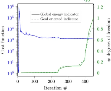
4.6 Cost function (solid) and number of degrees of freedom (dashed) evolutions for the L-bracket design problem. . . 80

4.7 Compliant mechanism design domain. Dimensions in mm. . . 81

4.8 Optimized compliant mechanism design with no stress constraint shows only thresholded volume fractions ˜ν greater than 0.8. . . 82

4.9 Von Mises stress field for the compliant mechanism design with no stress constraint. . . 83

4.10 Optimized compliant mechanism design with stress constraint ofσy = 0.15 shows only thresh-olded volume fractions ˜ν greater than 0.8. . . 84

4.11 Von Mises stress field for the compliant mechanism design with stress constraint. . . 85

4.12 Cost function (solid) and number of degrees of freedom (dashed) evolutions for compliant mechanism designs without (a) and with (b) stress constraint. . . 85

(11)

Chapter 1

Introduction

Topology optimization is a growing field that has found applications in many arenas, from the aerospace and automotive industries to microfluidics. It is a design tool that finds the optimal distribution of material in a design domain to minimize a cost function subject to a set of constraint inequalities. It is a relatively new approach to design which obviates the need for trial-and-error design and lessens the need for engineering intuition. Notably, it can be applied to design systems where intuition is lacking.

The first applications of topology optimization were in solid mechanics where the goal was to minimize a structure’s compliance subject to a constraint on its mass. In real world applications, however, structural components need to satisfy failure constraints related to maximum stress so as to prevent collapse. To satisfy these constraints, a redesign step of the compliance optimized design is performed, thereby reverting to the trial-and-error approach we want to avoid. Including these constraints directly in the optimization would render these redesign steps unnecessary. However, before this can be done, the accuracy of the computed stress field in the topology optimization must be increased; this thesis addresses this topic.

In topology optimization, the design geometry can be represented with volume fraction or level set methods. The volume fraction method discretizes the design domain into elements and assigns a volume fraction variable which ranges between 0 and 1 to each element. Penalization is used to enforce discrete values, i.e. either 0 or 1. Although this penalization method can nucleate holes, it is highly dependent of the problem and not always applicable. On the other hand, level set methods represent the design boundary implicitly using the isocontour of the scalar-valued level-set function. The design is discrete from the start hence penalization methods are unnecessary. However, the ability to change the topology is limited as new holes in the design are not created without external tools such as the topological derivative. In this thesis, we focus on the former method as it is well established in our field of application, i.e., linear elasticity.

The topology optimization problem is ill-posed, as the “optimal” designs consist of a non converging sequence of structures with highly oscillatory material-void regions. By far the most popular way to formulate a well-posed problem is by restriction whereby the oscillations are supressed by applying a filter operation to the volume fractions. This filter, however, blurs the boundary and renders the stress field inaccurate. To

(12)

obtain a sharp boundary, a threshold function over the volume fractions is commonly employed, however, the stress field inaccuracy is still not resolved.

Adaptive Mesh Refinement (AMR) refines (coarsens) the mesh in the domain regions with the highest (lowest) error of the approximated response is. This strategy allows us to save computational resources while increasing accuracy. It is ideally suited for topology optimization in which regions devoid of material are meaningless and need not be accurately modeled. The AMR would coarsen these regions. By the same token, regions filled with material require a higher mesh resolution for more accurate geometry definition and stress prediction.

In Chapter 2, we combine an AMR strategy with a thresholding function to obtain sharp boundaries and accurately computed stress fields. First, we perform a validation study to demonstrate the accuracy of the computed stress field by our AMR approach that is based on an energy error indicator. Next, we replace the energy error indicator with a goal oriented error indicator that is more suitable for our computed optimization cost and constraint functions. In this way, we attain suitably accurate cost and constraint function values, which ensures the design prototypes will behave as expected.

Chapter 3 explains the mesh dependency in the optimized designs that can result when viewing the design volume fraction field as an element of an Euclidean space rather than its proper function space. Problems arise when this approach is applied over nonuniform meshes, such as those generated in AMR. To address this issue, we first present an in-depth mathematical formulation of optimization algorithms in function spaces. Then, we lay out the necessary concepts to formulate optimization algorithms independent of the mesh configuration and apply them to one of the most popular algorithms in topology optimization, the Globally Convergent Method of Moving Asymptotes (GCMMA).

Chapter 4 leverages the concepts introduced in Chapters 2 and 3 to extend the range of applications to high resolution three dimensional designs. We also mention additional issues that need to be addressed to solve such large scale problems. Namely, the use of an efficient technique to filter the volume fractions across several mesh refinement levels and efficient preconditioners for the iterative linear solvers for multiple systems of equations.

(13)

Chapter 2

Adaptive mesh refinement in

stress-constrained topology

optimization

2.1

Introduction

Topology optimization is a well established design tool that has found industrial applications in recent years. However, most developments focus on the “compliance problem”, i.e. to minimize compliance subject to a mass constraint. This is in spite of the fact that in many cases, it is necessary to satisfy failure constraints such as on maximum yield stress. In this work, we investigate stress constrained topology optimization.

There are numerous challenges to solve stress-constrained problems. First, the optimal stress constrained solutions belong to degenerate lower dimension subspaces of the design domain. Gradient-based optimiza-tion algorithms cannot reach these optima; rather they get trapped in locally optimal soluoptimiza-tions. This phenomenon, first studied in the optimal design of trusses [27, 52, 92] is known in the literature as the “singularity problem”. It is resolved by relaxing the stress constraints, thereby regularizing the degenerate subspace [25, 77] . This is accomplished viaε−relaxation[26] orqp−relaxation[19] and the relaxed stress indicator [56]. In this work, we employ the last.

Second, the local stress constraints in the continuum setting lead to one constraint per finite element after discretization. This creates a scenario where the number of design variables is as large as the number of constraints, which is a computationally challenging problem. To overcome this, the constraints are agglomerated into a single measure that approximates the maximum stress value over the domain. These approximations include thep-norm and the Kreisselmeier-Steinhauser (KS) functions [73]. Alternatively, in [10] a ramp function is used to penalize all regions with stress constraint violations. We adopt this approach. Third, the inaccuracy of the computed stress field leads to designs that do not perform in service as their simulations suggest. This is because topology optimization does not use a conforming mesh; rather, it projects the design onto a fixed grid akin to a fictitious domain finite element method. Although this approach is convenient for the optimization, it yields poor accuracy in the computed response. This issue is exasperated in density-based topology optimization because the domain geometry is not explicitly defined; rather it is defined by an interphase of “partially filled” finite elements which renders useless stress computations. In

(14)

this work, we use Adaptive Mesh Refinement (AMR) and thresholding to obtain accurate stress values. Our goals are to obtain comparable optimal designs to those that are obtained on highly refined uniform meshes, compute accurate stress fields and reduce the computational cost. To achieve these goals we need a reliable and efficient error indicator to drive the AMR and a topology optimization strategy that accommodates the evolving discretization.

The first application of AMR in topology optimization appears in [63]; it uses separate design and analysis meshes which are related by a smoothing algorithm. The AMR is only performed on the analysis mesh; it is based on geometric criteria and no coarsening is performed. Coarsening is considered in [100] which uses a mesh hierarchy to solve the compliance problem. Again the refinement and coarsening criteria are solely based on the geometry and not on the error in the computed response. A similar approach proposed in [67] uses the distance function with respect to the domain boundary as the refinement and coarsening indicator. A study of the effects of various AMR parameters on the optimization performance appears in [71]. As in [63], they use different design and analysis meshes and as in [67], the AMR uses a geometric error indicator that is based on the proximity to the domain boundary. In [68], the AMR uses a tree data structure with polygonal elements; again the error indicator is solely based on geometrical considerations. Following this trend, [85] uses the phase-field method and refines regions adjacent to the design boundary.

Independently discretizing the design and analysis meshes, [102] refines each with their own error indi-cators to solve the compliance problem. Unfortunately, this approach is not scalable because it is necessary to perform a search over the design discretization for each finite element in the analysis mesh. On a pos-itive note, a posteriori error estimators are used to obtain accurate displacement and stress fields. In [20] two different error estimators are invoked to control error in the geometry and compliance. However, their method is only applied to compliance problems. An energy based error indicator is used in [97] to refine the mesh in the compliance problem. In the context of stress-constrained problems, [29] utilizes h-adaptive mesh refinement by combining mesh quality and displacement based error indicators. However, they do not validate the accuracy of their stress fields. [49] solves a stress constrained compliance minimization problem using an anisotropic mesh adaptation scheme based on the metric tensors of the spatial Hessian of the cost and constraint functions. Using topological derivatives [10] considers local stress constraints and develops an AMR method that is based on residual error indicators of the energy norm of the displacement.

Finite element analysis in structural topology optimization is a delicate issue, especially in regard to the calculation of the stress fields. Indeed, stress fields are not accurately resolved with the density method due to the blurred boundary region. Because of this, topology optimized designs are post processed wherein the blurred boundary is thresholded to define an “exact” boundary, a conforming mesh is created from this

(15)

boundary and shape optimization is used to obtain designs with desirable stress distributions. To eliminate the shape optimization task, [91] embeds stress field post-processing into the topology optimization wherein the interior stress values are extrapolated to the boundary region to compute more accurate stress fields. Another option to obtain accurate stress fields is to define an explicit domain boundary with the level set method and use either a conforming mesh [8, 59, 103] or eXtended Finite Element Method (XFEM) and sim-ilar approaches [41, 42, 83, 108] to capture the boundary. However, level-set methods cannot systematically nucleate holes and their designs are highly dependent on the initial design, which limits their effectiveness in comparison to density methods. It is possible to nucleate holes via topological derivatives; however, this approach is only practical for linear problems. It is also well known that level set methods suffer from poor convergence rates and numerical oscillations in the boundary [37]. They are also difficult to implement. However, for stress-constrained problems, they are immune to the singularity issue because there is virtually no blurred boundary region.

Our contribution is a topology optimization framework to obtain designs that satisfy pointwise stress constraints with a high degree of accuracy. We are able to achieve this goal by combining AMR and a thresholding function to obtain a sharp interphase that models the material boundary.

We implement our topology optimization framework on top of the parallel finite element library libMesh [51], which allows us to address large scale problems. This framework accomodates arbitrary cost and constraint functions and can be extended to other physics than elasticity. The high performance capability will be essential when solving problems in three dimensions, which is the scope of our future work.

2.2

Adaptive mesh refinement in stress-constrained topology

optimization

Topology optimization finds the distribution of material within a hold-all domainD that minimizes a cost function and satisfies constraints. Its mathematical statement is as follows

min

χ∈{0,1}θ0(χ) =

Z

D

π(χ,u)dV , (2.1)

s.t.u∈Vsatisfiesa(χ;u,v) =L(v) for all v∈V , (2.2)

θi(χ) = Z D gi(χ,u)dV ≤0 i= 1, 2...ni, (2.3) where a(χ;u,v) = Z χC[∇u]· ∇vdV (2.4)

(16)

and

L(v) =

Z

ΓN

t·vda. (2.5)

In the above, χ is the material indicator function defined such that χ(x) = 1 and χ(x) = 0 represents the presence or lack of material at x∈D, θ0 is the cost function to be minimized, e.g. compliance, mean displacement, maximum stress, etc. andθi are theni inequality constraint functions that typically limit the total mass, maximum stress, etc. In addition, the design needs to satisfy the linear elasticity equation, given in its weak form in Equation (2.2) whereuis the displacement field andV =

v∈H1₍_D₎d _| _v_{= 0 on ΓD} is the function space of admissible displacements, where ΓD is the boundary of D over which Dirichlet boundary conditions u = 0 are applied. ΓN is the complementary boundary of ∂D over which the non-homogeneous tractiontis applied; both ΓDand ΓN are fixed surfaces. Finally,Cis the symmetric elasticity tensor.

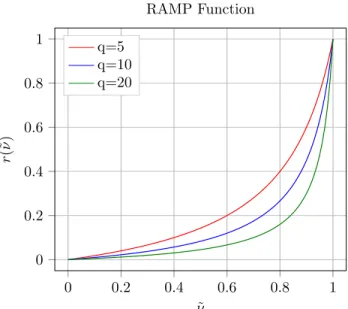
Our discrete optimization problem is not amenable to gradient-based algorithms. For this reason, we 1) convexify the design domain by replacing the binary-valued design fieldχ∈ {0, 1}with the volume fraction field ν, which continuously varies from 0 to 1, i.e. ν ∈[ν, 1], and 2) penalize intermediate values so thatν best mimics the characteristic function χ. This ensures the elasticity problem is well-posed. In this work, we penalize the elasticity tensor by replacingχ in Equation (2.4) with the RAMP function [86]

r(ν) = ν 1 +q(1−ν),

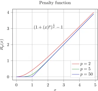
where q is the penalization parameter. Figure 2.1 plots the RAMP function for several values of q. We observe better behavior using the RAMP rather than the traditional SIMP method [16]. We use the usual ersatz material to model regions with no material, i.e., we replace regions whereχ(x) = 0 withν(x) =ν.

Unfortunately, the topology optimization problem is ill-posed. Compliance designs consist of a non converging sequence of structures with highly oscillatory material-void regions. There are two approaches to obtain a well-posed problem, relaxation and restriction. We use the restriction approach, wherein the design space is reduced by imposing a length scale constraint on the design’s geometric features. This is accomplished by imposing a constraint on the perimeter [43], the slope of the volume fraction field [74] or as in this work, by filtering the volume fraction field [17]. In this work, we use the cone filter presented in [21].

ˆ

ν(x,ν) =

Z

B(x)

(17)

0 0.2 0.4 0.6 0.8 1 0 0.2 0.4 0.6 0.8 1 ˜ ν r ( ˜ ν ) RAMP Function q=5 q=10 q=20

Figure 2.1: RAMP interpolation scheme.

whereB(x) is a ball of radiuscentered atxandK(x−y) is the cone kernel function, given by

K(p) =1

(− kpk) ifp∈ B(x) . (2.7)

The filter radiusis a parameter which defines the length scale such that the geometric complexity increases as → 0. It is important to consider the integral in Equation (2.6) instead of the weighted average of neighboring elements, as commonly seen in the literature, because the elements have different volume/areas when applying AMR. We considered using the PDE-based filter [55], but its solution with traditional lagrange elements requires a sufficiently refined mesh to avoid filtered volume fraction values above 1 and below 0. This is not possible at early stages of our AMR strategy. We will investigate in the future alternative methods that avoid this oscillation.

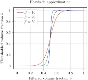
The filter operation brings an additional issue: the presence of blurred boundaries in the material inter-face. To lessen this effect, we use the threshold function of [98], cf. Equation (2.8),

˜

ν(ˆν) = tanh(0.5β) + tanh(β(ˆν−0.5))

tanh(0.5β) + tanh(β(1.0−0.5)), (2.8) whereβ is a parameter defined such that

lim

(18)

0 0.2 0.4 0.6 0.8 1 0 0.2 0.4 0.6 0.8 1

Filtered volume fraction ˜ν

Thresholded v olume fraction ˆ ν Heaviside approximation β = 10 β = 20 β = 50

Figure 2.2: Threshold function.

whereHis the unit step function. It is known that the threshold operation does not prevent the appearance of localized artifacts such as one-node-connected hinges in compliant problems, which can be alleaviated with a robust formulation [98] or with a stress constraint [31]. Therefore, we do not worry about features below the minimum length scale. The thresholding function makes the sensitivity zero in regions away from the ˜

ν= 0.5 level set boundary, which makes it difficult to nucleate holes. For this reason, we use a continuation approach whereinβ is selectively increased during the optimization.

Summarizing, we replace the binary material indicator fieldχwith the continuous volume fraction fieldν

to convexify the design space and make the optimization problem amenable to NLP. We compute the filtered volume fraction field ˆν to impose a length scale constraint and hence obtain a well-posed optimization problem. Finally we compute the thresholded volume fraction field ˜ν such that it mimics the originally sought material indicator functionχ. Ultimately we solve the topology optimization problem of finding ν

such that min ν∈[ν,1] θ0(ν) = Z D π(˜ν,u)dV , (2.10)

s.t.u∈Vsatisfiesa(ν;u,v) =L(v) for allv∈V, (2.11)

θi(ν) = Z D gi(˜ν,u)dV ≤0i= 1, 2..ni, (2.12) where a(ν;u,v) = Z D r(˜ν)C[∇u]· ∇vdV . (2.13)

(19)

2.3

Stress field accuracy in the density method

Convexifying the design space has the effect of blurring the domain boundaries, which creates inaccurate stress field computations, as demonstrated by [91]. In their work, sharper boundaries are obtained via a non-linear filter rather than the cone filter of Equation (2.6). Because of the mesh resolution, however, the boundary is jagged which gives rise to artificially high stress values. To resolve this jaggedness, the stress fields are post-processed by extrapolating the interior values onto the boundary.

In this work, we demonstrate that stress post-processing is not necessary if the mesh is adaptively refined leaving only a fine interphase boundary region. To validate our method, we perform the dog-bone study of [91] cf. Figure 2.3 in which D = 1m and r = 1/3 m. The material Young’s modulus is E = 10P a and the Poisson ratio, ν = 0.3. The volume fraction field that defines the plane stress structure is discretized as piecewise constant over the elements. The geometry is directly interpolated onto the mesh, i.e. only the elements whose centroidsxi are within the structure boundary take a ν(xi) = 1 volume fraction. For all other void elements we assignν(xi) =ν = 10−5. We then filter the volume fraction with Equation (2.6) and = 0.0625 m and thresholded with Equation (2.8) using β = 100 to leave a fine interphase region with intermediate volume fraction values. We apply uniaxial loading of 10 Pa significantly distant from the notches to avoid end effects in the notch region. Our calculated minimum principal stress is compared to those from empirical formulas [106]. This computation is repeated for several dog-bone orientations within the fixed mesh. In Figure 2.5, we plot the minimum principal stress across section A-A that passes through the center of the notch where it is seen that stress converges to the same distribution regardless of the orientation. The minimum principal stress value is−39.8, which is similar to the tabulated value−39.02 in [106].

To obtain these results, we use the residual based error indicator of Equation (2.35) and the Dörfler marking strategy [33] which is proven to decrease the error in elliptic problems. Unlike the marking strategy that we will employ in the optimization, the Dörfler strategy does not allow for coarsening. In our Dörfler implementation we select a subsetMof elements with minimum cardinality such that

ηM= X K∈M η_K2 !1/2 ≥θη θ∈[0, 1] , (2.14) where η= X K∈Th η_K2 !1/2 (2.15) andηK is the element error of Equation (2.35) andθ= 0.3. The mesh is iteratively refined until the total

(20)

energy errorη of Equation (2.38) is below 0.5. Figure 2.4 shows the refined mesh for an orientation of 0.4.

Figure 2.3: Dog-bone structure from [106].

2.4

Stress constrained topology optimization

Now we are in a position to formulate our topology optimization problem. We intend to minimize the volume of the structure subject to a constraint on the von Mises stress

σV M = r 3 2σ dev_·_σdev_, _(2.16) where σdev=σ−1 3(trσ)I (2.17)

is the deviatoric stress. As such the topology optimization problem now reads

min ν∈[ν,1] θ0(ν) = Z D ˜ ν dV, (2.18)

s.t.u∈Vsatisfiesa(ν;u,v) =L(v) for allv∈V, (2.19) andθ1(ν) =σV M ≤σy for allx∈D, (2.20)

whereσy is the maximum allowed stress.

A consistent numerical approach would use the same elasticity tensor for the displacement solution and the stress evaluation. However, [34] showed that the stress field in a porous micro structure tends to a non-zero value even when the volume fraction tends to zero. To be physically accurate, the stress field in regions with intermediate volume fraction ν ∈ [ν, 1] should therefore tend to non-zero values asν tends

(21)

Figure 2.4: Dog-bone structure and the mesh used in the analysis for an orientation of 0.4 radians. −0.4 −0.2 0 0.2 0.4 −40 −30 −20 −10 0 x2 Principal stress

Principal stress across section A-A

0.00 0.40 0.70 1.00 1.40

(22)

0 0.2 0.4 0.6 0.8 1 0 0.2 0.4 0.6 0.8 1 ˜ ν ηc ( ˜ ν ) Stress interpolation q= 2 q= 10 q= 50

Figure 2.6: Stress penalization function.

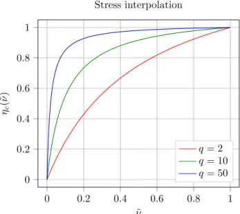
to zero. However, our focus is in obtaining black-and-white designs so we are not interested in accurately calculating the stress in regions with intermediate volume fraction. Therefore, when computing the stress we use a relaxed stress formulation similar to [56] wherein

C(˜ν) =ηc(˜ν)C0, (2.21)

whereηc is the inverse RAMP function

ηc(˜ν) = ˜ν 1 +q

1 +qν˜, (2.22)

cf. Figure 2.6. Basically, when computing the displacement in regions with intermediate volume fraction, we penalize_Csuch that it is more compliant which generates a displacement field which is artificially “large”. We now combine this large displacement field with a stiff _C to compute an artificially large stress field. Because of the volume minimization, the optimizer deems such regions inefficient and hence reduces their size.

The stress constraint Equation (2.20) is a pointwise constraint. When solving the elasticity equation using the finite element method, the pointwise constraint translates into one constraint per finite element; it is evaluated at the element centroidxi. This results in a computationally challenging optimization problem. To resolve this burden, the pointwise constraintsσV M(xi)≤σy are replaced by the single global maximum constraint max

xi

(23)

algorithm. As such aggregation strategies in [34, 104] approximate the maximum value of the Von Mises stress field with a p-norm or a Kreisselmeier-Steinhauser (KS) function [40]. Obviously the single global measure cannot represent the pointwise field values. To address this shortcoming, several strategies employ regional measures [47, 56, 72], where the single agglomerated constraint over the entire domain is replaced by several such constraints over subdomains. Another shortcoming with these aggregated measures is that they only approximate the maximum field value. A renormalization strategy was presented in [56] to improve the approximation. However, this approach results in a non-differentiable constraint although the effect of the non-differentiability lessens as the optimization converges.

We apply a different aggregation strategy that is commonly used in PDE-constrained optimization [46] and in [10] for stress constrained optimization via the topological derivative. It requires neither renormaliza-tion nor regional clustering techniques. We replace the pointwise constraint Equarenormaliza-tion (2.20) with the global constraintkσV M −σyk₊=

R

DR( σV M

σy )dV whereRis the shifted ramp function: R(x) =x−1 ifx >1 and

R(x) = 0 otherwise. For the optimization, we replace the ramp function with a smooth approximation Rp such that

Rp(x) = (1 + (x)p)p1 −_{1 ,} _(2.23)

cf. Figure 2.7. In our calculations, we usep= 8 and leave it constant throughout the optimization.

The constraint of Equation (2.23) is enforced via a penalty method with a penalty parameterγ so that the topology optimization problem now reads

min ν∈(0,1] θ0(ν) = Z D ˜ ν dV +γkσV M −σyk₊ , (2.24)

s.t.u∈Vsatisfiesa(ν;u,v) =L(v) for allv∈V. (2.25)

The parameterγis increased throughout the optimization, starting from a small value. This helps alleviate the sharp gradient in Equation (2.23).

We use an adjoint sensitivity analysis to evaluate the variation of a general functional θ(ν). Although this derivation is well-known, it behooves us to present it as it also plays a role in our AMR.

We use a reduced space optimization formulation, hence we must consider dependency ofuon the design variableν, i.e. u→u(ν) so that ˆθ(ν) =θ(ν,u(ν)). In this way

(24)

0 1 2 3 4 5 0 1 2 3 4 (1 + (x)p₎1p−₁ x Rp ( x ) Penalty function p= 2 p= 5 p= 50

Figure 2.7: Smoothed shifted function.

where δθˆ(ν;δν) is the variation of ˆθ at ν acting on δν; δuθ is the variation of θ at uacting on δu, δνθ is the variation ofθ at ν acting onδν andδuis the variation of uatν acting onδν. In the adjoint method, we annihilate the implicit variationδu(ν;δν). To do this we take the variation of the state Equation (2.25) with respect to the design fieldν and augment this zero term toδθˆ.

δθˆ(ν;δν) =δνθ(ν,u(ν);δν) (2.27) +δuθ(ν,u(ν);δu(ν;δν)) (2.28)

−δνa(u,v;δν) (2.29)

−δua(u,v;δu(ν;δν)) , (2.30)

whereδνaandδuaare the variations of the bilinear formawith respect to ν andu. In our linear elasticity

formulation

δua(u,v;δu(ν;δν)) =a(v,δu(ν;δν)) , (2.31) and

δνa(u,v;δu(ν;δν)) =

Z

D

(25)

To annihilateδu(ν;δν) in Equation (2.30), we define the arbitraryv∈V such that

a(v,δu) =δuθ(ν,u(ν);δu) for all δu∈V, (2.33)

where we use the symmetry of the bilinear froma. Having calculatedv,δθˆreduces to.

δθˆ(ν;δν) =δνθ(ν,u(ν);δν)−δνa(u,v,δν) . (2.34)

Summarizing, to calculate δθˆ(ν), we first solve the primal problem of Equation (2.25) to obtain u, we compute the partial derivative informationδuθ(ν,u(ν);δu) andδνθ(ν,u(ν);δν), we solve the adjoint problem of Equation (2.33) forvand finally we compute the variationδθˆfrom Equation (2.34).

2.4.1

Adaptive mesh refinement

To produce meaningful designs, we must compute the stress field with as much accuracy and efficiency as possible, hence the motivation to use AMR. More importantly, in optimization, AMR also provides an accurate and efficient means to compute the cost and constraint functions. Indeed, the engineer is basing the entire design on the values of these functions so their computed values must be accurate.

The accuracy of our finite element computation is directly dependent on the spatial discretization. To gauge this accuracy we compute an error measure which allows us to best allocate the spatial discretization parameters while simultaneously achieving the desired accuracy. In the context of finite element methods, these measures are called a posteriori error estimates. They bound the error in terms of the current solution approximation and are computed by summing the element error indicators over the mesh. In ourh-refinement AMR strategy, a marking strategy identifies the elements with largest and smallest errors for refinement and coarsening. The elements to be refined are divided in four children elements, which belong to a different refinement level, cf. Figure 2.8. Those elements to be coarsened are removed along with the corresponding children from the same parent, cf. Figure 2.9. The refinement creates so called “hanging nodes” that break the continuity of the displacement field. To ensure continuity, constraints are imposed that relate these nodes’ displacements to their parents’. We only allow for hanging nodes between children and their parents neighbors; i.e. not between children and their grandparents neighbors. Such situations are corrected by adding more elements, cf. Figure 2.10.

As just mentioned, the AMR strategy relies on element error indicators. The theory of a posteriori finite element error estimation for elliptic problems is well established cf. the monographs [6, 95]. The a posteriori error estimates are categorized into three types: explicit based error estimates, implicit

(26)

residual-Refinement

Figure 2.8: Element marked for refinement in red and the resulting refinement with now two levels.

Coarsening

Figure 2.9: Element marked for coarsening in blue and the coarsening result.

based error estimates and gradient or flux recovery based error estimates. The explicit and implicit methods approximate the error with the current finite element solution. The explicit estimates are easy to implement, however they render bounds with problem dependent constants that can be difficult to assign. The implicit estimates require the solution of multiple regional boundary value problems over single elements or small element patches. The problem dependent constants are avoided at the behest of additional computational expense and onerous implementations. Error estimates based on gradient or flux recovery post-process the finite element displacement field uh to obtain an improved approximation of the stress field ˆσ(uh) which is smooth and has better convergence properties versus the nominally computed discontinuous stress field σ(uh). The element error indicator is based on the difference between ˆσ(uh) andσ(uh). The most popular flux recovery method is the Zienkiewicz-Zhu [111, 112], which locally projectsσ(uh) onto a higher-order polynomial approximation space over a patch of neighboring elements. Its popularity is due to its easy implementation, generality and accuracy. However, it is well known that adaptive mesh refinement algorithms using this estimator are not effective for interface problems, e.g. such as those encountered in topology optimization problems [24, 70]. This is because the tangential components of the stress field

t·σt, wheretis any vector perpendicular to the interface normal vector, are discontinuous at the interface. Smoothing these components results in unnecessary overrefinement. Knowing that the stress field exists in theH(div,D) ={v ∈L2(D,Rn) : div v ∈L2(D)} space, [24] projects the stress field onto finite elements in this space. However, we do not follow this approach because H(div,D) finite elements are notoriously difficult to implement, especially in parallel computing environments.

(27)

Figure 2.10: Allowed hanging nodes green and disallowed hanging nodes in red (top) and additional refine-ment to resolve disallowed hanging nodes (bottom).

[94] wherein the element error indicator for an elementK∈ Th, where Th is the finite element mesh, is

ηK ={h2Kk∇ ·σ(uh) +fk 2 L2_(K) +1 2 X E∈E(K) hEkj(σ(uh)·n)k 2 L2(E)} 1/2_. _(2.35)

In the above, the stress field is computed as

σ(uh) =r(˜ν)_C[∇uh] (2.36) and j(σ·n)E=        Jσ(uh)·nK E /∈ ED,EN tN−σ(uh)·n E∈ EN (2.37)

is the traction jump across the element face E, which belongs to the set of faces of element K, E(K). ED⊂ΓDis the set of element faces with prescribed Dirichlet boundary condition andEN ⊂ΓN is the set of element faces with prescribedtN Neumann boundary condition. hK is the element diameter andhE is the element face area.

(28)

Summing the element errorηK gives the global error η= X K∈Th η2_K !1/2 . (2.38)

This in turn is used to compute upper and lower bounds on the energy norm of the error, i.e.

|||u−uh|||=

Z

D

r(ˆν)C[∇(u−uh)]· ∇(u−uh) dV . (2.39)

The upper boundCηwhereC is a constant ensures that the error estimate is conservative, i.e.

|||u−uh||| ≤Cη. (2.40)

On the other hand, the lower boundcη, wherecis also a constant, ensures the error estimate is not excessively conservative, i.e.

cη≤ |||u−uh|||. (2.41)

To refine the mesh, we use the element error indicator ηK, cf. Equation (2.35). Refinement (coarsening) is done in those elements whose error is above the 70-th percentile (below the 5-th percentile) of the error indicator distribution.

Conventional error estimates are based on global measures such as the energy norm as in Equation (2.39) or the L2_-norm _k_u₋_u_hk

L2. However these measures are not effective as we are only interested in accuracy of our optimization cost and constraint functions. For this purpose, goal-oriented error estimates were developed [14, 69]. As alluded to above, these estimates require the solution of the adjoint problem, which within our optimization context we have already solved to obtain the sensitivities.

To present the goal estimate, we discretizeu, i.e. we now finduh∈Vh such that

a(uh,vh) =L(vh) for allvh∈Vh, (2.42)

whereVh is the finite element discretization of the function spaceV. Substracting Equation (2.11) from this and noting thatVh⊆V yields the Galerkin orthogonality condition.

a(u−uh,vh) = 0∀vh∈Vh, (2.43)

(29)

We are interested in defining the error θ(u)−θ(uh) in a goal functional θ(u) :V → R, i.e. a cost or constraint function. We start by restating the adjoint problem in Equation (2.33). Dropping the argument

ν for conciseness and replacing δuwithw we findv∈V such that

a(v,w) =δuθ(u;w) for allw∈V . (2.44)

Expandingθ(u)−θ(uh) in first-order Taylor series and applying Equation (2.44) we find

θ(u)−θ(uh) =θ(u)−θ(u+uh−u) , (2.45) =θ(u)−θ(u)−δuθ(u;uh−u) −okuh−uk 2 , (2.46) =δuθ(u;uh−u) , (2.47) =a(v,u−uh) , (2.48) =a(u−uh,v) . (2.49)

Equation (2.49)1_{gives us the error estimate for the quantity of interest}_θ_{, however, the exact adjoint solution}

v is unknown, rather we compute vh using the discretization that is used to compute uh, but this yields a zero error estimate by Galerkin orthogonality of (2.43). A common technique to resolve this issue is to calculate vh over a more refined mesh or to post-processvh to obtain a higher order approximation. We instead follow [38] and add the zero Galerkin orthogonality Equation (2.43) to Equation (2.49) and apply Cauchy-Schwarz inequality to obtain bounds on the error.

θ(u)−θ(uh) =a(u−uh,v−vh) , (2.50) = Z D r(ˆν)_C[∇(u−uh)] ·[∇(v−vh)]dV , (2.51) ≤ p r(ˆν)C[∇(u−uh)] _L2 × p r(ˆν)_C[∇(v−vh)] _L2 , (2.52) =|||u−uh||||||v−vh|||. (2.53) 1_{In Equation (2.47), we have neglected the higher order terms. For details on higher order nonlinear functionals, we refer} to [14].

(30)

With these bounds, we can reformulate the error estimate in terms of the energy norms: θ(u)−θ(uh)≤ |||u−uh||||||v−vh|||, (2.54) ≤ X K∈Th |||u−uh|||_K|||v−vh|||_K, (2.55) eK =|||u−uh|||K|||v−vh|||K. (2.56)

The expression inside the summation is the K element error indicator Equation (2.56) which is used to mark cells for refinement and coarsening throughout the optimization. We compute the error indicator |||u−uh|||K =ηK from Equations (2.35)–(2.36). The estimate for |||v−vh|||K is similarly computed using Equations (2.35)–(2.36), but we replaceuh withvh andf and tN with their corresponding body load and traction from the adjoint linear term δuθ. With the error indicator eK for each element, we proceed as in the energy error approach and refine the elements whose error is above the 70-th percentile of the error indicators distribution and coarsen those below the 5th percentile. We only use the element error indicator (2.56) and not the goal estimate (2.55), as it is not accurate [38].

2.4.2

Optimization algorithm and refinement strategy

Our optimization framework uses the C++ MMA [89] implementation by [3]. We implement a continuation strategy for the β parameter in the threshold function Equation (2.8) and for the penalty parameterγ in Equation (2.25). We do not wait for MMA to converge to change these parameters, rather we increase them following a heuristic strategy.

For each optimization iteration k, we use the current design estimateνk to calculate the state uh and adjointvh states, which are needed to calculate the costθ0 and constraintθi functions and their gradients ∇θ0 and∇θi for (i= 1, ...,ni). These are fed into the optimizer which then updates the design toνk+1, cf. Algorithm 1. During each optimization iteration, we determine if the relative change in the cost function between iterations is smaller thantolAM R. If so, we invoke our AMR strategy described earlier. The MMA mesh dependent information, i.e. the design field and Lagrangian multiplier variables over the last three iterations [89], are interpolated onto the new mesh. Next, the filter kernel is reconstructed. We update the threshold and penalty parameters β and γ following a heuristic strategy explained in the numerical examples. Finally,tolAM Ris updated such that its value is halved after each refinement. We resettolAM R to its starting value once the threshold parameter β exceeds 200 so as to reinitiate the refinement. The termination criteria for the optimization is based on the change in the design or the maximum number of iterations, set to 500.

(31)

Algorithm 1Algorithm outline. 1: Build filter.

2: while kνk−νk+1k> tolorit < maxitdo

3: Solve state problem to obtainu

4: Solve adjoint problem to obtainv

5: Calculateθ0(νk),∇θ0(νk)

6: Updateνk+1 according to the MMA algorithm. 7: if θ0(νk)−θ0(νk+1)

θ0(ν) ≤tolAM Rthen 8: Calculate ηK forK= 1...nel

9: Sort element errors in decreasing order.

10: Refine of 30 % of the elements with highest errors. 11: Coarsen of 5 % of the elements with lowest errors. 12: Update filter with the new mesh.

13: Project MMA data into the new discretization. 14: UpdatetolAM R

15: end if

16: if β satisfiesβ-criteriathen

17: Updateβ

18: end if

19: if γ satisfiesγ-criteriathen

20: Updateγ

21: end if

22: end while

2.4.3

Finite Element Implementation

The finite element computations are performed in parallel thanks to the libMesh finite element library [51]. For solvers we use PETSc [12, 13], and the HYPRE [60] preconditioner. As both the adjoint and primal problems share the same stiffness matrix, we recycle the preconditioner to avoid the overhead of multiple builds. libMesh uses a quadtree/octree data structure in their adaptive mesh refinement implementation. We use bilinear Lagrangian elements and accomodate the hanging nodes via constraint equations. Our code design is similar to that in [38] wherein the users need only write the optimization cost and constraint functions and their derivatives with respect touandν. All the optimizations were run on a 8-core 2.60 GHz Intel Xeon E5-2670 processor.

2.4.4

Numerical examples

We first benchmark our algorithm with the eyebar example from [10]. The design domain in Figure 2.11 is discretized with the Gmsh library [28] using second order triangles to capture the circumference with more precision and avoid sharp angles when refining the mesh. The largest triangle has an inradius of 0.15 mm and the smallest, 0.10 mm, placed near the hole. The load applied on the left hand side of the hole follows the distributiont(x,y) = (−((y−4)2_−1.52_{), 0.0) and Dirichlet boundary conditions are applied to the 2 mm}

(32)

segment in the right side. The isotropic material has a Young’s modulusE= 1.0 MPa, a Poisson’s ratio of

ν = 0.3 and a yield criteria isσy= 5 M P a. The filter radius is= 0.6mm. The initial mesh contains 681 elements. We limit the maximum refinement level to four because the relatively large filter radius compared to the mesh dimensions causes the filter kernel to exhaust the computer’s memory if the refinement is too high. 8 4 16 4 1.5 2 y x

Figure 2.11: Gray design domain, loads and boundary conditions. All dimensions are in mm.

Our continuation strategy to obtain optimized designs is as follows. First, the threshold parameter β

starts with a value of 1 and is increased by 5 every 20 iterations after iteration 50 to avoid having the design fall into a local minimum. Second, the penalty parameterγ starts with a value of 10 and is increased by 50 every 50 iterations after iteration 50. The tolerance to trigger refinementtolAMR is 1e-2.

We plot the optimized design in Figure 2.12. As we can see, part of the structure is stuck to the right side of the hole. The reason being that, thanks to the threshold function of Equation (2.8), the sensitivities are only significant in the material-void transition regions, i.e. at the design boundaries. If the hold-all domain boundary∂D coincides with the intended design domain boundary, it is difficult to move the latter, as the sensitivity is zero there because the design boundary interface cannot fully resolve itself. For this reason we expand the domain into the hole, cf. Figure 2.13. To recover the intended design domain, we impose a zero volume constraint for the thresholded volume fractions ˜ν in the extended, i.e. red, region.

(33)

Figure 2.13: Initial mesh with extended simulation domain in red.

We plot the new design in Figure 2.14. The nonlocal nature of the filter causes the zero volume constraint to extend its influence beyond the actual hole. To resolve this, in the extended domain, we equate ν = 0 and= 0 to avoid nonzero filtered volume fractions within the hole.

We first run an optimization using the global energy norm error indicator described in Section 2.4.1. The result with this approach cf. Figure 2.15, shows how the algorithm fails to obtain a complete 0/1 design. Indeed, the lack of a global convergence mechanism in MMA causes an oscillatory behavior in the boundary region near the hole. We also plot the Von Mises Stress field in Figure 2.16. The optimization time was 1900.8 seconds, out of which 339.5 seconds were devoted to the filter kernel construction.

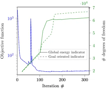
Using the same parameters as the previous case, we run an optimization using the goal-oriented error indicator with respect to the cost function, cf. Equation (2.24). The new optimized design in Figure 2.17 is almost identical to that obtained with the global energy error indicator, cf. Figure 2.15. The optimization took 1893.6 seconds, with 313.91 devoted to the filter kernel. The evolution of the cost function is similar as well, but the refinement process is not, cf. Figure 2.18. The goal error indicator initially refines fewer elements than the energy error where after it refines more until the difference stagnates due to the ceiling on the maximum level of refinement. The upticks in the value of the cost function correspond to mesh refinements, which resulted in higher stress values.

(34)

Figure 2.15: Optimized design for the eyebar geometry with the global energy error indicator andν= 0 and

= 0 in the extended simulation domain.

Figure 2.16: Von Mises stress field for the eyebar design in Figure 2.15.

Figure 2.17: Optimized design for the eyebar geometry with the goal-oriented error indicator andν= 0 and

= 0 in the extended simulation domain.

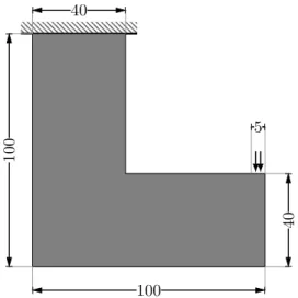
For the sake of comparison, we study the “L-bracket” problem described in [56], cf. Figure 2.19. We apply 0.08 N/mm traction over the load region, the isotropic material model has again a Young’s modulus ofE = 1.0 MPa , Poisson’s ratio ofν= 0.3 andν = 10−4; the filter radius is= 2.0 mm and the maximum allowable Von Mises stress is σy = 2 MPa. The initial design uses the mesh in Figure 2.20 which defines refinement level 0.

Again, there are several knobs that need to be adjusted to obtain the optimized design. First, the threshold parameterβ in Equation (2.8) starts with a value of 1 and is not increased until iteration number

(35)

0 100 200 300 102 103 Iteration # Ob jec ti v e function

Global energy indicator Goal oriented indicator

0 100 200 300 2 3 4 5 6 7 ·104 Iteration # # degrees of freedom

Figure 2.18: Cost function and discretization degrees of freedom histories for the eyebar.

100. Thereafter then increased by 5 every 20 iterations up to a maximum value of 250. This is necessary to obtain a sharp interface and also prevents the design from falling into local minima. Second, the penalty parameterγstarts with an initial value of 1 and increases by 2 every 20 iterations after iteration 50. Third, the maximum refinement level is fixed at 3 until iteration 200, 5 until iteration 400, and 8 thereafter. These strategies give us the best results. For example, it prevents areas with intermediate volume fraction values from being overly refined given that they are eliminated with the threshold function later in the optimization. The tolerance to trigger the refinementtolAM Ris initially 1e-2; it is halved after each refinement. As such

tolAM Rcan become very small early in the design process, i.e. while the primary topology is still evolving. This is attributed to the threshold function, which makes the problem similar to a shape optimization. Therefore, we resettolAM R=1e-2 every 80 iterations after iteration 100.

As in the previous example, we extend the simulation domain beyond the design domain, cf. the red region in Figure 2.20. We likewise equateν = 0 and= 0 in these red areas. This approach however, does not work well for the L-bracket problem. As seen in Figure 2.21, there is still part of the material stuck at the L-bracket corner. The corner creates a high stress concentration, but the gradient is zero there due to the threshold operation in (2.8), as explained earlier. For this reason, we revert to our previous approach and place a zero constraint on thresholded volume fractions ˜ν in the extended region; we no longer have

ν = 0 and = 0. As in Figure 2.20 design, we run an optimization using the global energy norm error indicator described in Section 2.4.1. Our result in Figure 2.22 shows an optimized design with a volume of 1228.49 mm2_{. The final mesh contains 524,842 elements. The same mesh with a uniform refinement}

(36)

100

40

5

Figure 2.19: Gray design domain, loads and boundary conditions.. All dimensions are in mm.

Figure 2.20: Initial mesh for the optimization and actual design domain shown in gray. A zero volume constraint is imposed in the extended domain shown in red.

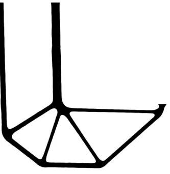
We plot the Von Mises stress distribution calculated using the SIMP stress formula given in the weak form in Equation (2.13), i.e. σ=r(˜ν)_C[∇u], cf. Figure 2.23. The distribution is considerably more uniform, which indicates a more optimized design. We plot the mesh corresponding to the optimized design with different zoom levels in Figure 2.26. Note the high refinement level that it is necessary to accurately compute the stress field.

The total computational cost was of 2181.6 seconds. Out of this time, 797.2 seconds were devoted on building the cone filter in Equation (2.6). This expensive operation is done every time the mesh is refined

(37)

Figure 2.21: Optimized design usingν = 0 and= 0 in the extended region.

Figure 2.22: Optimized design using zero volume constraint on the thresholded volume fractions in the extended region.

and has an algorithmic complexity that is polynomial with respect to the number of elements. Based on this, it is even more compeling to find out a way to use [55] in the context of AMR.

Using the same parameters as the previous case, we run another optimization but we replace the global energy error indicator for the goal-oriented error indicator, cf. Equation (2.24) to obtain the best possible accuracy. The optimized design is similar than that obtained with the global energy error indicator, cf.

(38)

Figure 2.23: Von Mises stress for the design of Figure 2.22.

Figures 2.22 and 2.24. The total volume is 1233.01 mm2 _{and the mesh contains 516,346 elements which is} less than those obtained via the global energy error indicator.

The goal-oriented optimization took 2120.4 seconds. Figure 2.25 shows the evolution of the cost function and the number of degrees of freedom for the displacement field. The goal oriented error indicator marks fewer elements for refinement than the energy error indicator which translates into a slight computational saving for our case. The global nature of the goal error, Equation (2.24), explains the similar number of elements versus the energy error. A cost function localized in a small region would have resulted in a more localized mesh refinement because the adjoint response would only be significant in the small region.

2.4.5

Design validation with explicit geometry finite element simulation

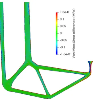
To validate the Figure 2.22 design, we use the ˜ν = 0.5 level set of the thresholded volume fraction field to define the optimized geometry. A body-fitted mesh is genererated over this domain and a finite element analysis is performed to compute the displacement and stress fields using the finite element library FEniCS [9]. We plot the difference between the fitted and topology optimized (topopt) Von Mises stress fields

σfitted_{V M} −σtopopt_{V M} , cf. Figure 2.27. As we can see, most of the difference is within 10% of the maximum von mises stress value of 2 MPa, withσtopopt_{V M} slightly greater thanσ_{V M}fitted.

For comparison purposes, we run a similar optimization with a single uniform mesh containing 528,384 elements, which is similar to the number of elements in the optimal design of Figure 2.22. This result is

(39)

Figure 2.24: Optimized design using the goal oriented error indicator. 0 100 200 300 400 100 101 102 103 104 105 106 Iteration # Cost function

Global energy indicator Goal oriented indicator

0 100 200 300 400 0 0.2 0.4 0.6 0.8 1 1.2 ·106 Iteration # # degrees of freedom

Figure 2.25: Cost function and discretization degrees of freedom histories for the L-bracket.

plotted in Figure 2.28 with a total volume of 1381.9mm2_{. We perform a similar validation study with a body} fitted mesh and plot the result in Figure 2.29, as expected the lack of refinement creates a greater difference in the Von Mises stress field over the design boundaries and in the thin structural members. Increasing the refinement with two additional levels to match the most refined elements in our AMR mesh will improve the stress field, but this uniform mesh would result in 8,454,144 elements, versus the 524,842 elements in our AMR mesh.

(40)

2.5

Conclusion and future work

We presented a new topology optimization methodology to obtain designs in structural mechanics with accurate stress fields that satisfy yield criteria. We are able to do so by combining a threshold function that sharpens the otherwise blurred boundaries from the filter operation and adaptive mesh refinement that increases the mesh resolution in the boundary region. We validated the stress accuracy by using geometries whose stress fields are known and tabulated. The eye-bar and L-bracket example problems are used to validate our approach. We foresee that it is possible to further improve our results by using a globally convergence optimization algorithm such as the GCMMA [90] and the PDE-based filter [55] to reduce memory requirements.

Future work will address a more rigurous mesh refinement strategies. One that considers the inexactness of the finite element approximation and still ensures global convergence to a local minima [109]. This will avoid our current heuristic and case dependent strategy, e.g. for the assignment of β,tolAM R, etc. Indeed for this approach to be succesful, it is necessary to employ error estimates and error indicators with tighter bounds than the currently used residual based approaches. To save computational resources, uncoupling the discretizations of the volume fraction field and the displacement field could be incorporated.

(41)

(42)

Figure 2.27: Von Mises stress field verification.

(43)

(44)

Chapter 3

Mesh independency in topology

optimization

3.1

Introduction

Topology optimization finds the optimal distribution of material in a given design domainDto minimize a cost function and satisfy constraint function inequalities. On a background mesh that represents the design domain, the optimization algorithm places material in individual elements to define the geometry of the optimal design. Regions devoid of material are meaningless, hence the motivation to coarsen the mesh in these regions. By the same token, regions which contain material require a higher mesh resolution. This cost saving strategy that distributes elements with different sizes within the mesh is known as the Adaptive Mesh Refinement (AMR).

In the usual topology optimization scenario, the design is defined by an element-wise material volume fraction. This piecewise uniform function, i.e. design field, belongs to the Hilbert space L2 defined on

D, i.e. L2(D). If the elements have differente sizes, as in AMR, it is intuitively wrong to think that all design variables have the same contribution to the sensitivities. Here we explain why it is also necessary to accomodate the element size when calculating the inner products involving the design variables within the optimization algorithms. However, this is not done within most optimization algorithms used in the topology optimization community as they assume the design is a vector in the Euclidean space`2, i.e., simply a vector of length equal to the number of elements in the mesh, cf. IPOPT [96], SNOPT [39], MMA [89], FMINCON [62] and Optimality Criteria [44]. On the other hand, the optimization libraries Optizelle [105], Moola [84], ROL [76] and TAO [32] contain to various extents the capacity of treating design fields as elements of their underlying function spaces. Related work by [81] compares mesh-independent and dependent versions of the steepest descent algorithms for an unconstrained problem and estimates their rates of convergence. It is also necessary to mention that in the PDE-constrained optimization community, optimization algorithms are inherently mesh-independent as they are implemented in the corresponding function space. For instance, [93] implements an infinite-dimensional (inf-dim) primal-dual interior-point method with a Newton solver and [110] implements an inexact sequential quadratic programming method with an adaptive multilevel

(45)

mesh refinement scheme.

The inconsistency between theL2and`2spaces is generally not a problem because most of the topology optimization studies use uniform meshes. However, when using meshes with different element sizes, as is the case in AMR, the`2 viewpoint yields mesh dependent designs, whereas theL2 approach does not.

This work is laid out as follows: Section 3.2 presents the mathematical tools we need to implement mesh independent optimization algorithms. We use these tools in Section 3.3 to make one of the most popular optimization algorithms in the topology optimization community, the Globally Convergent Method of Moving Asymptotes (GCMMA/MMA) algorithm, mesh independent. In Section 3.4, we validate our theory by solving three common problems in topology optimization. Section 3.5 briefly summarizes our findings and presents conclusions.

3.2

Mathematical Preliminaries

Our topology optimization algorithm becomes mesh independent by being formulated in the inf-dim L2 space, using concepts from functional analysis. It is then discretized in a consistent manner using the finite element space of the discretized design field, i.e. the element-wise uniform volume fraction field. Notably, the norms in the optimization algorithm that check for convergence are discretized in this finite element space.

To illustrate the proper discretization, consider the unconstrained minimization problem

min ν∈V θ(ν) ,

(3.1)

with the functional

θ:V 7→R, (3.2)

where ν : V 7→ R is our volume fraction design field that belongs to V, a Hilbert space on domain D, equipped with an inner product (·,·)V, which induces the primal normk·kV. For our topology optimization,

V =L2(D); it is equipped with the norm

kνk_L2 =p(ν,ν)L₂= Z D ν2 dV 1/2 . (3.3)

(46)

the space of linear operators fromV toR, i.e. V∗⊂L(V,R). Both the primalk·kV and dualk·kV∗ norms

can be used to check for convergence in optimization algorithms.

To formulate optimization algorithms on the function space V, we need the Riesz map from the Riesz representation theorem: LetV be a Hilbert space with inner product (·,·)V and dual spaceV∗. For every

ϕ∈V∗ there is a unique elementu∈V such thatϕ(v) = (u,v)_V for allv∈V. This one-to-one map is the Riesz map Φ :V 7→V∗ defined such that Φ(u) =ϕ.

The discretization of the primal and dual spaces follows from [82]. We approximate the volume fraction field ν ∈ V with νh ∈ Vh, where Vh is the span of basis functions P ={φ1, ...,φn}, φi ∈ V and n is the dimension ofVh. Our approximation now reads

νh(x) = n

X

i=1

νiφi(x) =νTφ(x) . (3.4)

Replacingν withνh and similarlyι∈V withιh∈Vh in the inner product definition yields

(νh,ιh)V_h= Z D (νTφ)(ιTφ)dV =νT Z D φφT dV ι =νTMι, (3.5) where M= Z D φφT dV (3.6)

is the mass matrix that reflects the mesh discretization. By construction,Mis symmetric and invertible. The discretized design fieldνhis in the function spaceVh= (Rn, (·,·)M), i.e. vectors of dimensionnwith

anMinner product. This inner product induces the normkνhk_V

h =kνkM= (ν

T_M_ν₎1/2_. Clearly the L2 norm kνhkL2 = (ν

T_M_ν₎1/2 _{differs from the} _`

2 norm kνhk`2 = (ν

T_ν₎1/2_{. In topology} optimization, νh is usually discretized via piecewise uniform functions over the individual elements so M is a diagonal matrix whose entries are the volumes (areas) in 3D (2D) of each element in the mesh. So if the mesh is uniform, M is simply the identity matrix times the element volume (area) Ve and hence kνhkL2 =Vekνhk`2.

The basis P induces a unique dual basis P∗ = {φ∗₁, ...,φ_n∗} for V_h∗ defined such that φ∗_i ∈ V∗ and

(47)

ιh∈Vh Fh(ιh) = n X i=1 Fiφ∗i(ιh) . (3.7)

In this way,Fh(ιh) is computed as

Fh(ιh) = n X i=1 Fiφ∗i   n X j=1 ιjφj  , = n X i=1 Fj n X j=1 ιjφ∗i(φj) , = n X i=1 Fiιi, =FTι, (3.8)

where we used the orthonormal property between the bases P and P∗ and the linearity ofF. From the Riesz representation th