A very simple safe-Bayesian random forest

A Very Simple Safe-Bayesian Random Forest

Novi Quadrianto and Zoubin Ghahramani

Abstract—Random forests works by averaging several predictions of de-correlated trees. We show a conceptually radical approach to generate a random forest: random sampling of many trees from a prior distribution, and subsequently performing a weighted ensemble of predictive probabilities. Our approach uses priors that allow sampling of decision trees even before looking at the data, and a power likelihood that explores the space spanned by combination of decision trees. While each tree performs Bayesian inference to compute its predictions, our aggregation procedure uses the power likelihood rather than the likelihood and is therefore strictly speaking not Bayesian. Nonetheless, we refer to it as a Bayesian random forest but with a built-in safety. The safeness comes as it has good predictive performance even if the underlying probabilistic model is wrong. We demonstrate empirically that our Safe-Bayesian random forest outperforms MCMC or SMC based Bayesian decision trees in term of speed and accuracy, and achieves competitive performance to entropy or Gini optimised random forest, yet is very simple to construct. Index Terms—Bayesian methods, random forest, decision trees

F

1

INTRODUCTION

Decision trees [1] represent a classical induction method that is widely used. This is because decision trees exhibit many appealing properties: they are sim-ple to understand and interpret, applicable for both classification and regression tasks, and offer good predictive performance. Although defining a global objective to optimally learn decision trees is funda-mentally hard, there are several approaches to learn trees based on Gini impurity [1] and information-theoretic considerations [2], [3].

Breiman [4] used an ensemble of unpruned Gini-optimiseddecision trees to improve the performance of learning. This random forest framework has become a very popular and powerful tool with applications ranging from machine learning, computer vision, computer graphics, to medical image analysis, among others [5], [6]. For a recent comprehensive survey about random forests, refer to [7]. The randomness is introduced during training phase of the trees via: a) random sampling of the training dataset [4], and b) partitioning the data space with only randomised subsets of data features [8]. We will call trees trained with this procedure as randomly trained trees. An important ingredient of random forest is the compo-sition of trees that are randomly different from one another. This results in de-correlated individual tree predictions and, therefore, in an improved generalisa-tion. The notion of randomness helps the model to be robust with respect to noisy data.

Reflecting on how a random forest is built from • N. Quadrianto is with SMiLe CLiNiC, Department of Informatics,

University of Sussex, UK. E-mail: [email protected] • Z. Ghahramani is with Department of Engineering, University of

Cambridge, Cambridge, UK. Email: [email protected] Manuscript received May 2013.

randomly trained trees, we ask the following natural question: can we simplysample many treesfrom some prior distributions, and perform an ensembleof those randomly sampled trees? The Bayesian framework is a principled way to achieve this. We note that the usage of Bayesian statistics for learning decision trees has a long history of successful methods, among others, [9], [10], [11], [12], [13], [14].

Bayesian approaches start by defining a prior dis-tribution on the space of decision trees. Subsequently, a likelihood function, for example Gaussian (for re-gression tasks) or Bernoulli (for classification tasks), is evaluated within each data block induced by the decision tree. The likelihood describes the conditional distribution of the output data given input data falling into the corresponding block. Inall previous models using Bayesian statistics, the prior distribution of the decision tree is defined conditionally on the given input data. Sophisticated Markov Chain Monte Carlo (MCMC) methods [11] or sequential Monte Carlo [14] is then used to approximate intractable posterior computations. In this paper, we will show a novel usage of a prior that allows us to sample decision trees even before looking at the data.

As more data arrives, Bayesian decision trees will put a mass to a single tree. This is a desired be-haviour of Bayesian model averaging [15]. We are instead interested to explore ensemble of trees in the sense of model combination [16]. We achieve this by borrowing the concept of power likelihood [17], [18]. By utilising a data independent prior coupled with the power likelihood, we deliver fast yet safe Bayesian random forests that exceed the performance of Bayesian decision trees and are competitive with random forests and SVMs. We use the notion of Safe-Bayesian from [19] in a reference to procedures based on a so-calledβ-Bayesian posterior (power likelihood

several binary and multi-class classification problems. Finally, Section 6 concludes the paper.

2

THE

MODEL

Here we describe our model of Safe-Bayesian ran-dom forest. Assume that we are given input X =

{x1, . . . ,xN} with xi ∈ X = RD and output Y =

{y1, . . . , yN} with yi ∈ Y = {1, . . . , C}. The goal is

to infer a function F : X → Y that maps inputs to outputs. In this paper, we only focus on the clas-sification tasks. We are interested in the case where the latent function is anensembleof predictors, where each predictor partitions the input data space into axis-aligned blocks. Note that the partitioning can be represented graphically as adecision tree.

To elaborate the form of our Safe-Bayesian random forest model, we begin by establishing notation and model for a single tree. LetT be a rooted and strictly binary tree; a tree that has a single root node, internal nodes with exactly two outgoing edges (also known as children), and terminal (leaf) nodes. Each node of the tree v ∈ T corresponds to a block Bv ⊂ RD,

and has a splitting rule applied onBv. The rule splits

the block Bv into two halves: Bvl and Bvr associated

with the left and right child nodes, respectively. The splitting rule is characterised by the dimension of the split, κv ∈ {1, . . . , D}, and the location of the

split (also known as cut value), τv. Thus, we have

Bvl =Bv∩ {x∈RD :xκv ≤τv}, andBvr=Bv∩ {x∈

RD : xκv > τv}. Note that the root node has a

block B(root) = _RD_{, and terminal nodes do not}

have splitting rules associated to them. Each terminal node however describes conditional distribution of the labels given all input data falling into that node. We will denote a decision tree with tree structure, split dimensions, and split values as T = {T, κ, τ}. Our Bayesian analysis proceeds by specifying a prior probability distribution on the space of decision trees, that isp(T).

2.1 Tree Priorp(T)

In defining a prior on decision trees, we note that the dimension of the split κ, and the location of the split τ serve as an index for the splitting rule of each T. It is then more convenient to exploit the relationship that p(T, κ, τ) = p(κ, τ|T)p(T), and specify p(κ, τ|T)

and p(T) separately. We discuss the specifications of p(T)and p(κ, τ|T) in the subsequent sections.

A generative process of trees structurep(T)

codes are generated in depth-first order starting from

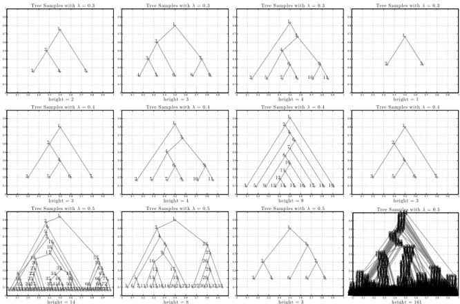
1 at the root node. Refer to Figure 1 for examples of tree coding, and to Figure 2 for samples of different trees structures.

A prior on cut dimensions and valuesp(κ, τ|T)

Given the structure of the tree, we will then need to specify the splitting rules for each of the internal nodes of the tree. For internal nodev, the dimension κv and location τv of the cut are chosen uniformly

from{1, . . . , D}and [0,1], respectively. That is κv ∼ U({1, . . . , D}) (1)

τv ∼ U([0,1]). (2)

We have assumed that the input features at each dimension lie in[0,1]. We will describe in Section 5 on how to enforce this.

Note that our prior on the space of decision trees defined above isindependentof the data X. Once we generate the structure of the tree, and fill up the in-ternal nodes with splitting rules, we have completely specified the decision tree. This is in contrast to exist-ing work on Bayesian decision trees, for example [11], [13], [14]. Under the Chipman et al. model that is the model used in these existing works, the probability that a nodevis split into two children isαs/(1 +|v|)βs

with the parameters αs ∈ (0,1) and βs ∈ [0,∞)

governing the shape of the resulting tree, and |v| is the depth of the node. For largerαsandβsthe typical

trees are larger, while deeperv is in the tree the less likely it will be split. This is in fact a data-independent tree structure prior. However, as noted in [14], given the data at a particular internal node, the split di-mension and location are sampled from the uniform distribution over the available data features and data values. Therefore, for all Bayesian decision trees, the probability of tree growing, and the distribution of the split dimension and location, depend on X so that every node in the tree will contain at least one data point. [14] put forward the theoretical need for data independent priors over the space of decision trees that include tree structures, cut dimensions and values to make the model coherent with respect to changing dataset sizes. On the practical side, the effect of data independent prior enables us to use exactly the same trees structures in all our experiments. We have just defined a way to partition the data, the next required thing is to define a conditional distribution of the labels given input data falling into corresponding blocks. This is described in the next section.

Fig. 1:Coding of a rooted and strictly binary tree. Internal nodes are denoted with circles and terminal nodes with squares. Each internal node has exactly two outgoing edges. The code for an internal node is1 and0 is for a terminal node. Codes are generated in depth-first order starting from1 at the root node.

0 0.1 0.2 0.3 0.4 0.5 0.6 0.7 0.8 0.9 1 0 0.1 0.2 0.3 0.4 0.5 0.6 0.7 0.8 0.9 1 height = 2 1 2 3 4 5

Tree Samples withλ= 0.3

0 0.1 0.2 0.3 0.4 0.5 0.6 0.7 0.8 0.9 1 0 0.1 0.2 0.3 0.4 0.5 0.6 0.7 0.8 0.9 1 height = 3 1 2 3 4 5 6 7 8 9

Tree Samples withλ= 0.3

0 0.1 0.2 0.3 0.4 0.5 0.6 0.7 0.8 0.9 1 0 0.1 0.2 0.3 0.4 0.5 0.6 0.7 0.8 0.9 1 height = 4 1 2 3 4 5 6 7 8 9 10 11

Tree Samples withλ= 0.3

0 0.1 0.2 0.3 0.4 0.5 0.6 0.7 0.8 0.9 1 0 0.1 0.2 0.3 0.4 0.5 0.6 0.7 0.8 0.9 1 height = 1 1 2 3

Tree Samples withλ= 0.3

0 0.1 0.2 0.3 0.4 0.5 0.6 0.7 0.8 0.9 1 0 0.1 0.2 0.3 0.4 0.5 0.6 0.7 0.8 0.9 1 height = 3 1 2 3 4 5 6 7

Tree Samples withλ= 0.4

0 0.1 0.2 0.3 0.4 0.5 0.6 0.7 0.8 0.9 1 0 0.1 0.2 0.3 0.4 0.5 0.6 0.7 0.8 0.9 1 height = 4 1 2 3 4 5 6 7 8 9 10 11 Tree Samples withλ= 0.4

0 0.1 0.2 0.3 0.4 0.5 0.6 0.7 0.8 0.9 1 0 0.1 0.2 0.3 0.4 0.5 0.6 0.7 0.8 0.9 1 height = 9 1 2 3 4 5 6 7 8 9 10 11 12 13 14 15 16 17 18 19

Tree Samples withλ= 0.4

0 0.1 0.2 0.3 0.4 0.5 0.6 0.7 0.8 0.9 1 0 0.1 0.2 0.3 0.4 0.5 0.6 0.7 0.8 0.9 1 height = 3 1 2 3 4 5 6 7

Tree Samples withλ= 0.4

0 0.1 0.2 0.3 0.4 0.5 0.6 0.7 0.8 0.9 1 0 0.1 0.2 0.3 0.4 0.5 0.6 0.7 0.8 0.9 1 height = 14 1 2 3 4 5 6 7 8 9 10 11 12 1314 15 16 17 18 19 20 21 22 23 24 2526 27 2829303132 33 34 35 36 37 3839 40 41 4243 44 4546 47 48 49 50 515253545556 57 58 59 60 6162 63 64 65 66 67 68 6970 71 72 737475 Tree Samples withλ= 0.5

0 0.1 0.2 0.3 0.4 0.5 0.6 0.7 0.8 0.9 1 0 0.1 0.2 0.3 0.4 0.5 0.6 0.7 0.8 0.9 1 height = 8 1 2 3 4 5 6 7 8 9 10 11 12 13 14 15 16 17 18 19 20 21 22 23 24 25 26 27 28 29 30 31 32 33 Tree Samples withλ= 0.5

0 0.1 0.2 0.3 0.4 0.5 0.6 0.7 0.8 0.9 1 0 0.1 0.2 0.3 0.4 0.5 0.6 0.7 0.8 0.9 1 height = 3 1 2 3 4 5 6 7 8 9 Tree Samples withλ= 0.5

0 0.1 0.2 0.3 0.4 0.5 0.6 0.7 0.8 0.9 1 0 0.1 0.2 0.3 0.4 0.5 0.6 0.7 0.8 0.9 1 h ei ght = 161 1 2 3 4 5 6 7 8 9 10 11 12 13 14 15 16 17 18 19 20 21 22 23 24 25 26 27 28 29 30 31 32 33 34 35 36 37 38 39 40 41 42 43 44 45 46 47 48 49 50 51 52 53 54 55 56 57 58 59 60 61 62 63 64 65 66 67 68 69 70 71 72 73 74 75 76 77 78 79 8081828384 8586 87 888990919293949596979899 100 101 102 103 104 105 106 107119129128127108124123122120121118117109110111112113114115116143137142141140139138126136135134133132131130125144 145 146 147 148 149 150 151152 153 154 155 156 157 158 159171179178177176175174173172170160169168167166165164163162161180 181 182 183 184 185 186 187 188 189 190 191 192 193 194 195 196 197 198 199200201202 203 204 205 206 207 208 209 210 211 212 213 214 215 216 217 218 219 220 221 222 223 224 225 226 227 228 229 230 231 232 233 234 235 236 237 238 239 240 241 242 243 244 245 246247248249250251252 253 254 255 256 257 258 259 260 261 262 263 264 265 266 267 268 269 270 271 272 273 274 275 276 277 278 279 280 281 282 283 284 285 286 287 288 289 290 291 292 293 294 295 296 297 298 299 300 301 302 303 304 305 306 307 308 309 310 311 312 313 314 315 316 317318 319 320 321 322 323 324 325 326 327328329330331332333334 335 336 337 338 339 340 341 342 343 344 345 346 347 348 349 350 351 352 353 354 355 356 357 358 359 360361 362363 364374381380379378377376375373365372371370369368367366382 383 384 385 386 387 388 389 390 391 392 393 394 395 396 397398399400401402 403 404 405 406 407 408 409 410 411 412 413 414 415 416 417 418 419 420 421 422 423 424 425 426 427 428 429430431432 433 434 435451466464462460459458457456455436453452454450442437438449440441439443444445446447448461463465467468469470471472473 474 475 476 477 478 479 480 481 482 483 484 485 486 487 488 489 490 491 492 493 494 495 496 497 498 499 500 501 502 503 504 505 506 507 508 509 510511 512 513 514 515 516 517 518 519 520 521 522 523 524 525 526 527 528 529 530 531 532 533 534 535 536 537 538 539 540 541 542 543 544 545 546 547 548 549 550564575574551572571570569568567566565573563556562552554555553557558559560561587595594593592591590589588580586585584583582581579578577576596 597 598 599 600 601 602 603 604 605606 607608 609 610 611 612 613 614 615 616 617 618 619 620 621 622 623 624 625 626 627 628 629 630631 632633 634 635 636 637 638639640 641657669668667666665664663662661660659642658656648643644645646655647649650651652653654670671672673674 675 676 677 678 679 680 681 682 683 684 685 686 687 688 689 690 691 692 693 694 695 696 697 698 699 700 701 702 703 704 705 706 707 708 709 710 711 712 713 714 715 716 717 718 719 720 721 722 723 724 725 726 727 728 729 730 731 732 733 734 735 736 737 738 739 740 741 742 743 744 745 746 747 748 749 750 751 752 753 754 755 756 757 758 759 760 761 762 763 764 765 766 767 768 769 770 771 772773774 775 776 777 778 779 780 781 782 783809803804805806807808810801811812813784816817802815800791799785786788789790787792794795796797793798835832833834839836837838840830841831824829821814818828820819822823825826827842843844845846847 848 849 850 851 852 853 854 855 856 857 858 859 860 861 862 863 864 865 866 867 868 869 870 871 872 873 874 875 876 877 878 879 880 881908902903904905906907909900910911912882914915901913899889898883885886887888884890897892893894895896891932933934935936940937938939941943930931922929928927926925924923921920919918917916942944 945 946 947 948 949 950 951 952 953 954 955 956 957 958 959 960 961 962 963 964 965 966 967 968 969 970982990989988987986985984983981971980979978977976975974973972991 992 993 994 995 996 997 998 999 1000 1001 1002 1003 1004 1005 1006 1007 1008 1009 1010 1011 1012 1013 1014 1015 1016 1017 1018 1019 1020 1021 1022 1023 1024 1025 1026 1027 1028 1029 1030 1031 1032 1033 1034 1035 1036 1037 1038 1039 1040 1041 1042 10431044 1045 1046104710481049 1050 1051 1052 1053 1054 1055 1056 1057 1058 1059 1060 1061 1062 1063 1064 1065 1066 1067 1068 1069 1070 1071 1072 1073 1074 1075 1076 1077 1078 1079 1080 1081 1082 1083 108410851086 1087 1088 1089109010911092109310941095 1096 10971098 1099 1100 11011102 110311041105 1106 1107 1108 1109 1110 1111 1112 111311271138113711361135113411331132113111301129112811261114112511241123112211211120111911181117111611151139 1140 1141 1142 1143 1144 1145 1146 1147 1148 1149 1150 1151 1152 1153 1154 1155 1156 1157 1158 1159 1160 1161 1162 1163 1164 1165 1166 1167 1168 1169 1170 1171 1172 11731174 117511761177 1178 1179118011811182118311841185118611871188118911901191119211931194 1195 1196 1197 1198 1199 12001201 1202 1203 1204 1205 1206 1207 1208 1209 1210 1211 12121226123612351234123312321231123012291228122712251213122412231222122112201219121812171216121512141237 1238 1239 1240 1241 1242 1243 1244 1245 1246 1247 1248 12491250125112521253 1254127012831282128112801279127812771276127512741273127212711269125512681267126612651264126312621261126012591258125712561284 1285 1286 1287 1288 1289 1290 1291 1292 1293 12941309132113201319131813171316131513141313131213111310130812951307130613051304130313021301130012991298129712961322 1323 1324 1325 1326 1327 1328 1329 1330 1331 1332 1333 1334 1335 1336 1337 1338 1339 1340 1341 1342 1343 1344 1345 1346 1347 1348 1349 1350 1351 1352 1353 1354 1355 1356 1357 1358 1359 1360 136113661362136913701365136413631389138813801387138613851384138313821381137613791378137713751374137313721371136813671390 1391 1392 1393 1394 1395 1396 1397 1398 1399 1400 1401 1402 1403 1404 1405 1406 1407 1408 1409 1410 1411 1412 1413 1414 1415 1416 1417 1418 1419143114391438143714361435143414331432143014201429142814271426142514241423142214211440 1441 1442 1443 1444 1445 1446 1447 1448 1449 1450 1451 1452 1453 1454 1455 1456 1457 1458 1459 1460 1461 1462 1463 1464 1465 1466 1467 1468 1469 1470 1471 1472 1473 1474 1475 1476 1477 1478 1479 1480 1481 1482 1483 1484 1485 1486 1487 1488 1489 1490 1491 1492 14931494 1495 1496 1497 1498 1499 1500 1501 1502 1503 1504 1505 1506 1507 1508 1509 1510 1511 1512 1513 1514 1515 1516 1517 1518 1519 1520 1521 1522 1523 1524 1525 1526 1527 1528 1529 1530 1531 1532 1533 1534 1535 1536 1537 1538 1539 1540 1541 1542 1543 1544 1545 1546 1547 1548 1549 1550 1551 1552 1553 1554 1555 1556 1557 1558 1559 1560 1561 1562 1563 1564 1565 1566 1567 1568 1569 1570 1571 1572 1573 1574157515761577 1578 1579 1580 1581 1582 1583 1584 1585 1586 1587 1588 1589 1590 1591 1592 1593 1594 1595 1596 1597 1598 1599 1600 1601 1602 1603 1604 1605 1606 1607 1608 1609 1610 1611 1612 1613 16141615 16161617 1618 1619 1620 1621 1622 1623 1624 1625 1626 1627 1628 1629 1630 1631 1632 1633 1634 1635 1636 1637 1638 1639 1640 1641 1642 1643 1644 1645 1646 1647 1648 1649 1650 16511652 1653165416711670166916681667166616651664166316621661166016591658165716561655167216731674 1675 1676 1677 1678 1679 1680 1681 1682 1683 1684 1685 1686 1687 1688 1689 1690 1691 1692 1693 1694 1695 1696 1697 1698 1699 1700 1701 1702 1703 17041705 1706171617231722172117201719171817171715170717141713171217111710170917081724 1725 1726 1727 1728 1729 1730 1731 1732 1733 1734 1735 1736 1737 1738 1739 1740 1741 1742 1743 1744 1745 1746 1747 1748 1749 1750 1751 1752 1753 1754 1755 1756 175717581778177917801781178317841786177617871788178917911792179317771782177517661759176017741762176317641765176117671769177017711772177317681818181218131814181518161817182218191820182118231825182618101811179918091798178517901808179517961797179418001801180218031804180518061807185318451848184918511852185718541855185618431858185918601861184418501842183418241827182818301831183218331829183518371838183918411840183618811877187818791880188518821883188418861888187518761872187418651846187318621863186418471866186818691870187118671910190519061907190819091912191119031913191419151916190418931902189419011889189018911892188718951900189718981899189619321933193419351938193619371939194019411930193119231929192819271926192519241922192119201919191819171942 1943 1944 1945 1946 1947 1948 1949 1950 1951 1952 1953 1954 1955 1956 19571958 1959 19601961 196219631964 1965 1966 1967 1968196919701971197219731974 1975 1976 1977 1978 1979 1980 1981 1982 1983 1984 1985 1986 1987 1988 1989 1990 1991 1992 1993 1994 1995 1996 1997 1998 1999 2000 2001201920362035203420322029202820272026202520022023202220212020202420182009200320042005201720072008200620102012201320142015201620112041204520442043204220372040203920382033203120302046 2047 2048 2049 2050 2051 2052 2053 2054 2055 2056 2057 2058 2059 2060 2061 2062 2063 2064 20652066 20672068 2069 20702071 20722073 207420752076207720782079208020812082 2083 2084 2085 2086 2087 2088 2089 2090 2091 2092 2093 2094 2095 2096 2097 2098 2099 2100 2101 2102 2103 2104 2105 2106 2107 2108 21092110211121122113211421152116 2117 2118 2119 2120 2121 2122 2123 2124 2125 2126 2127 2128 2129 2130 2131 2132 2133 2134 2135 2136 213721382139 2140 2141 2142 2143 21442160214521782173217221712170216921672165216421632162216121662159215221472146215821482149215021512153215421552156215721932198219221942195219722072199220022012203220522092190219121962189218021682174217521772179217621812185218721822186218321842188221822332234223222282224222322222221222022192217221022022204221622082206221122122213221422152239224622452244224322422241224022362238223722252235223122302229222722262247 2248 2249 2250 2251 2252 2253 2254 2255 2256 2257 2258 2259 2260 2261 2262 2263 2264 2265 2266 22672268 2269 2270 2271 2272 2273 2274 2275 2276 2277 2278 2279 2280 2281 2282 2283 2284 2285 2286 2287 2288 2289 2290 2291 2292 2293 2294 2295 2296 2297 2298 2299 2300 2301 2302 2303230423052306 2307 2308 2309 2310 2311 2312 2313 2314 2315 2316 2317 2318 2319 2320 2321 2322 2323 2324 2325 2326 2327 2328 2329 2330 2331 2332 2333 2334 2335 2336 2337 2338 2339 23402341 23422343234423452346234723482349235023512352 2353 2354 2355 2356 2357 2358 2359 2360 2361 2362 2363 2364 2365 2366 2367 2368 2369 2370 2371 2372 2373 2374 2375 2376 2377 23782379 2380 2381 2382 2383 2384 2385 2386 2387 2388 2389 2390 2391 2392 2393 2394 2395 2396 2397 2398 2399 2400 2401 2402 2403 2404 2405 2406 2407 2408 2409 2410 2411 2412 2413 2414 2415 2416 2417 2418 2419 2420 2421 2422 2423 2424 2425 2426 2427 2428 2429 2430 2431 2432 2433 2434 2435 2436 2437 2438 2439 2440 2441 2442 2443 2444 2445 2446 2447 2448 2449 2450 2451 2452 2453 2454 2455 2456 2457 2458 2459 2460 2461 2462 2463 2464 2465 2466 2467 2468 2469 2470 2471 2472 2473 2474 2475 2476 2477 2478 2479 2480 2481 2482 24832484 2485 2486 2487 2488 2489 2490 2491 2492 2493 24942506251725142495251225112510250925082507251325052499250424962498249725002501250225032524253025292528252725262525251925232522252125202518251625152531 2532 2533 2534 2535 2536 2537 2538 2539 2540 2541 2542 2543 2544 2545 2546 2547 2548 2549 2550 2551 2552 2553 2554 2555 2556 2557 25582559 2560 2561 2562 2563 2564 2565 2566 2567 2568 2569 2570 2571 2572 2573 2574 2575 2576 2577 2578 2579 2580 2581 2582 2583 2584 2585 2586 2587 2588 2589 2590 2591 2592 2593 2594 2595 2596 25972598259926002601260226032604260526062607 2608 2609 2610 2611 2612 2613 2614 2615 2616 2617 2618 2619 2620 2621 2622 2623 2624 2625 2626 2627 2628 2629 2630 2631 2632 2633 2634 2635 2636 2637 2638 2639 2640 2641 2642 2643 2644 2645 2646 2647 2648 2649 2650 2651 2652 2653 2654 2655 2656 2657 2658 2659 2660 2661 2662 2663 2664 2665 2666 2667 2668 2669 2670 2671 2672 2673 2674 2675 2676 26772678 2679 2680 268126982712271127102709270827072706270527042703270227012700269926972682269626952694269326922691269026892688268726862685268426832713 2714 2715 2716 2717 2718 2719 2720 2721 2722 2723 2724 2725 2726 2727 2728 2729 2730 2731 2732 2733 2734 2735 2736 2737 2738 2739 2740 2741 2742 2743 2744 2745 2746 2747 2748 2749 2750 2751 2752 2753 2754 27552756275727582759276027612762 2763 2764 2765 2766 2767 2768 2769 2770 2771 2772 2773 2774 2775 2776 2777 2778 2779 2780 2781 2782 2783 2784 2785 2786 2787 2788 2789 279028002791280728062804280328022801280527992797279627952794279327982792282828242825282628272831282928302832283328222823281228212820281928182817281628152814281328112810280928082834 2835 2836 2837 2838 2839 2840 2841 2842 2843 2844 2845 2846 2847 2848 2849 2850 2851 2852 2853 2854 2855 2856 2857 2858 2859 2860 2861 2862 2863 2864 2865 2866 2867 2868 2869 2870 2871 2872 2873 2874 2875 2876 2877 2878 2879 2880 2881 2882 2883 2884 2885 2886 2887 2888 2889 2890 2891 2892 2893 2894 2895 2896 2897 28982899 29002901 29022903 2904 2905 2906290729082909291029112912291329142915 2916 2917 2918 2919 2920 2921 2922 2923 2924 2925 2926 2927 2928 2929 2930 2931 2932 2933 2934 2935 2936 2937 2938 2939 2940 2941 2942 2943 2944 2945 29462947294829492950295129522953 2954 2955 2956 2957 2958 2959 2960 2961 2962 2963 2964 2965 2966 2967 2968 2969 2970 2971 2972 2973 2974 2975 2976 29772978 29792980 2981 2982 2983 2984298529862987298829892990 2991 2992 2993 2994 2995 2996 2997 2998 2999 3000 3001 3002 3003 3004 3005 3006 3007 3008 3009 301030113012 30133014 3015 3016 3017 3018 3019 3020 3021 302230233024 30253026302730283029303030313032303330343035303630373038 3039 3040 3041 3042 3043 3044 3045 3046 3047 3048 3049 3050 3051 3052 3053 3054 3055 3056 3057 3058 3059 3060 3061 3062 3063 3064 3065 3066 3067 3068 3069 3070 3071 3072 3073 3074 3075 3076 3077 3078 30793097308031113110310931083107310631053104310331013100309930983102309630873081308230953084308530863083308830903091309230933094308931323128312931303131313631333134313531383141312631273137312531173124311331143115311631123118312031213122312331193165315931613162316331643168316631673169317031713157317231733158316031563146315531393140314231443145314331473149315031513152315331483154318931873188319331903191319231853186317631843183318231813180317931783177317531743194 3195 3196 31973198 319932003201 320232033204 320532213233323232313230322932283227322632253224322332223220320632193218321732163215321432133212321132103209320832073234 3235 3236 3237 3238 3239 3240 3241 3242 3243 3244 3245 3246 3247 3248 3249 3250 3251 3252 3253 3254 3255 3256 3257 3258 3259 3260 3261 3262 3263 3264 3265 3266 3267 3268326932703271 3272 3273 3274 3275 3276 3277 3278 3279 3280 3281 3282 3283 3284 3285 3286 3287 3288 3289 3290 3291 3292 3293 32943295 3296 3297 3298 3299 3300 3301 3302 3303 3304 3305 3306 3307 330833193327332633253324332333223321332033183309331733163315331433133312331133103328 3329 3330 3331 3332 3333 3334333533363337333833393340334133423343 3344 3345 3346 3347 3348 3349 3350 3351 3352 3353 3354 3355 3356 3357 3358 3359 3360 3361 3362 3363 3364 3365 3366 3367 3368 3369 3370 3371 3372 3373 3374 337533893400339933983397339633953394339333923391339033883376338733863385338433833382338133803379337833773401 3402 3403 3404 3405 3406 3407 3408 3409 3410 3411 3412 3413 3414 3415 3416 3417 3418 3419 3420 3421 3422 3423 3424 3425 3426 3427 3428 3429 3430 3431 3432 3433 3434 3435 34363437 3438 34393440344134423443 3444 3445 3446 3447 3448 3449 3450 3451 3452 3453 3454 3455 3456 3457 3458 3459 3460 3461 3462 3463 3464 3465 3466 3467 3468 3469 3470 3471 3472 34733474 34753476 34773494350835073506350535043503347835013500349934983497349634953502349334843492347934803481348334823485348634873488348934903491351835253524352335223521352035193510351735163515351435133512351135093526 3527 3528 3529 3530 3531 3532 35333534 35353536353735383539354035413542354335443545354635473548 3549 3550 3551 3552 3553 3554 3555 3556 3557 3558 3559 3560 3561 3562 3563 3564 3565 3566 3567 3568 3569 3570 3571 3572 3573 3574357535763577 357835893597359635953594359335923591359035883579358735863585358435833582358135803598 3599 3600 3601 3602 3603 3604 3605 3606 3607 3608 3609 3610 3611 3612 3613 3614 3615 3616 3617 3618 3619 3620 3621 3622 3623 3624 3625 3626 3627 3628 3629 3630 3631 3632 3633 3634 3635 3636 3637 3638 3639 3640 3641 3642 3643 3644 3645 3646 3647 3648 3649366136693668366736663665366436633662366036503659365836573656365536543653365236513670 3671 3672 3673 3674 3675 367636773678 3679 3680 3681 3682 3683 3684 3685 3686 3687 3688 3689 3690 3691 3692 3693 3694 3695 3696 3697 3698 3699 3700 3701 3702 3703 3704 3705 3706 3707 3708 3709 3710 3711 3712 3713 3714 3715 3716 3717 3718 3719 3720 3721 3722 3723 3724 3725 3726 3727 3728 3729 3730 3731 3732 3733 3734 3735 3736 3737 3738 3739 3740 3741 3742 3743 3744 3745 374637613772377137703769374737673766376537643763376237683760375237593748374937513750375337543755375637573758378237893788378737863785378437833775378137803779377837773776377437733790 3791 3792 3793 3794 3795 3796 3797 3798 3799 3800 3801 3802 3803 3804 38053806 38073808 3809 3810 3811 3812 3813 3814 3815 3816 3817 3818 3819 3820 3821 3822 3823 3824 3825 3826 3827 3828 3829 3830 3831 3832 3833 3834 3835 3836 3837 3838 3839 3840 3841 38423843384438453846 3847 3848 3849 3850 3851 3852 3853 3854 3855 3856 3857 3858 3859 3860 3861 3862 3863 3864 3865 3866 3867 38683869 3870 3871 3872 3873 3874 3875 3876 3877 3878 3879 388038813882388338843885388638873888388938903891 3892 3893 38943895 3896 3897 38983899 3900 3901 3902 3903392039043936393439333931393039293928392739263925392339223921392439193910390639073908391839093911391239133914391539163917390539523949395039513957395339553956394639473954394539393944393239353938393739403941394239433985397939803981397839823983398439913986398739883989399039923993399439963977397639753964394839583959396039743962396339613965397139663972397339703969396839673995399739983999400040014002400340044005 4006 4007 4008 4009 4010 4011 4012 4013 4014 4015 4016 4017 4018 4019 4020 4021 4022 4023 4024 4025 4026 4027 4028 4029 4030 4031 4032 4033 4034 4035 4036 4037 4038 4039 4040 4041 4042 4043 4044 4045 4046 4047 4048 4049 4050 4051 4052 4053 4054 4055 4056 4057 4058 4059 4060 4061 4062 4063 4064 4065 406640674068 4069 40704071 4072 4073 4074 40754076 407740784079408040814082408340844085408640874088 4089 4090 4091 4092 4093 4094 4095 4096 4097 4098 4099 4100 41014102 4103 4104 4105 4106 4107 4108 4109 4110 4111 4112412541134140413641334132413141294128412741264130412441184114411541234117411641194120412141224150416341624161416041574156415541544153415241514141414941474146414541444143414241394148413841374135413441664168416741594165416441584169 4170 4171 4172 4173 4174 4175 4176 4177 4178 4179 4180 4181 4182 4183 4184 4185 4186 4187 4188 4189 4190 4191 4192 4193 4194 4195 4196 4197 4198 4199421242224221422042194218421742164215421442134211420042104209420842074206420542044203420242014223 4224 4225 4226 4227 4228 4229 4230 4231 4232 4233 4234 42354236 42374238 4239 4240 4241 4242 4243 4244 4245 4246 4247 4248 4249 4250 4251 4252 4253 4254 4255 4256 4257 4258 4259 4260 4261 4262 4263 4264 4265 4266 4267 4268 4269 4270 4271 4272 4273 4274 4275 4276 4277 4278 4279 42804281 4282428342844285 4286 4287 4288 4289 4290 4291 4292 4293 4294 4295 4296 4297 4298 4299 4300 4301 4302 4303 4304 4305 4306 4307 4308 4309 4310 4311 4312 4313 4314 4315 4316 4317 4318 4319 4320 4321 4322 4323 43244341435443534325435143504349434843474346434543444343434243524340433143394326432843294330432743324338433443354336433743334370437143724373437643744375437743784368436943604367436643654364436343624361435943584357435643554379 4380 4381 4382 4383 4384 4385 4386 4387 4388 4389 4390 4391 4392 4393 4394 4395 4396 4397 4398 4399 4400 4401 4402 4403 4404 4405 4406 4407 4408 4409 4410 4411 4412 4413 4414 4415 4416 4417 441844194440443944384437443644354434443344324431443044294428442744264425442444234422442144204441444244434444 4445 4446 4447 4448 4449 4450 4451 4452 4453 4454 4455 4456 4457 4458 4459 4460 4461 4462 4463 4464 4465 4466 4467 4468 4469 4470 4471 4472447344744475447644774478447944804481448244834484448544864487 4488 4489 4490 4491 4492 4493 4494 4495 4496 4497 4498 4499 4500 4501 4502 4503 4504 4505 4506 4507 4508 4509 4510 4511 4512 45134514 4515 4516 4517 4518 4519 4520 4521 4522 4523 4524 4525 4526 4527 4528 4529 4530 4531 4532 4533 4534 4535 4536 4537 4538 4539 4540 4541 4542 4543 4544 45454546 45474548454945504551 45524561456745664565456445634562456045534559455845574556455545544568 4569 4570 4571 4572 4573 4574 4575 4576 4577 4578 4579 4580 4581 4582 4583 4584 4585 4586 4587 4588 4589460346144613461246114610460946084607460646054590460446024595459145924593460145944596459745984599460046154616461746184619 4620 4621 4622 4623 4624 4625 4626 4627 4628 4629 4630 4631 4632 4633 4634 4635 4636 4637 4638 4639 4640 4641 4642 4643 4644 4645 4646 4647 4648 4649 4650 4651 4652 4653 4654 4655 4656 4657 4658 4659 4660 4661 4662 4663 4664 4665 4666 4667 4668 4669 4670 4671 4672 4673 4674 4675 4676 4677 4678 4679 4680 46814682 4683 4684 4685 468646964687470447014700469946984697470746954693469246914690469446894688472147184719472047244722472347164725472647174712471547144713471147104709470847064705470347024727 4728 4729 4730 4731 4732 4733 4734 4735 4736 4737 4738 4739 4740 474147424743474447454746474747484749 4750 4751 4752 4753 4754 4755 4756 4757 4758 4759 4760 4761 4762 4763 4764 4765 4766 4767 4768 4769 4770 4771 4772 4773 4774 4775 47764777 4778 4779 4780 4781 4782 4783 4784 4785 4786 4787 4788 4789 4790 4791 4792 4793 4794 4795 4796 4797 4798 4799 4800 4801 4802 4803 4804 4805 4806 4807 4808 4809 4810 4811 4812 48134830481448504846484348404839483848374835483448334832483148364829482148174828481848194816482048224823482448254826482748154862486348644865486648674873486848694870487248744876486048614851485948484841485848424844484548474849485248534854485548564857488348884887488648854884487548824881488048794878487748714889 4890 4891 4892 4893 4894 4895 4896 4897 4898 4899 4900 4901 4902 4903 4904 4905 4906 4907 4908 4909 4910 4911 4912492849414940493849374913493549344933493249314930492949364927491949264914491549174918491649204921492249234924492549514959495849574956495549544953495249444950494949484947494649454943494249394960 4961 4962 4963 4964 4965 4966 4967 4968 4969 4970 4971 4972 4973 4974 4975 4976 4977 4978 4979 4980 4981 4982 4983 4984 4985 4986 4987 4988 4989 4990 4991 4992 4993 4994 4995 4996 4997 49984999500050015002500350045005500650075008 5009 5010 5011 5012 5013 5014 5015 5016 5017 5018 5019 5020 5021 5022 5023 5024 5025 5026 5027 5028 5029 5030 5031 5032 5033 5034 5035 5036 5037 5038 5039 5040 5041 5042 5043 5044505750675066506550645063506250615060505950585056504550555054505350525051505050495048504750465068 5069 5070 5071 5072 5073 5074 5075 5076 5077 507850795080 50815082508350845085508650875088 5089 5090 5091 5092 5093 5094 5095 5096 5097 5098 5099 5100 5101 5102 5103 5104 5105 5106 5107 5108 5109 5110 5111 5112 5113 5114 5115 5116 5117 5118513051385137513651355134513351325131512951195128512751265125512451235122512151205139 5140 5141 5142 5143 5144 5145 5146 5147 5148 5149 5150 5151 5152 5153 5154 5155 5156 5157 5158 5159 5160 5161 5162 5163 5164 5165 5166 5167 5168 5169 5170 5171 5172 5173 5174 5175 5176 5177 5178 5179 5180 5181 518251835209520852075206520552045203520252015200519951985197519651955194519351925191519051895188518751865185518452105211 Tree Samples withλ= 0.5

Fig. 2:Sampling trees structures from the prior atλ∈ {0.3,0.4,0.5}. Once we generate the structures, and fill

up the internal nodes with splitting rules, we will completely specify decision trees.

2.2 Dirichlet-Multinomial Tree Likelihood

p(Y|X,T)

To specify a predictive model within each block, we follow the Bayesian model of [9], [11]. We will repeat them here for the self consistency of the paper. For an input vector x that falls into the ν-th terminal node, we assign a parametric family f indexed by

θν, f(y|θν), that models the conditional distribution

y|x. For a classification problem where the output y belongs to one of C classes {1, . . . , C}, the natu-ral choice for f(y|θν) is a multinomial distribution

with conjugate Dirichlet prior on terminal node pa-rameters. Given a block partitioning and a predic-tive model within each partition, we assume that y values within a terminal node are i.i.d. given θν

and y values across terminal nodes are independent.

Thus the form of class conditional distribution at a particular node v for a specific decision tree T

is f(YNv|XNv,θ,T) = Qi∈Nv

QC

c=1θ

I[yi=c ]

c , where

θ = (θ1, . . . , θC), θ>1 = 1, and θc ≥ 0 for all

c∈ {1, . . . , C}. As well, for simplicity of presentation, we have denoted as Nv the set of indices of the

input vectors that fall into partition blockBv, that is

Nv = {i : xi ∈ Bv}. Thus, XNv and YNv are input

vectors and their labels in block Bv, respectively. In

the above, we make use of Iverson’s bracket notation:

I[P] = 1 for the condition P is true and it is 0

otherwise. We put a conjugate Dirichlet prior on θ

with parameterα= (α1, . . . , αC),αc>0, and assume

conditional independence of parameters across termi-nal nodes. Thus, we have the following likelihood: p(Y|X,T) = R Q_v∈Ω

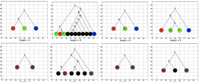
Fig. 3:A visualisation of4trees with the highest (top row) and4trees with the lowest (bottom row) importance weights for a 3-class problem ‘iris’ dataset (best viewed in colour). The terminal nodes are colour encoded according to the label proportions of data points falling into the terminal nodes. The three colours, red, green, and blue, correspond to the three class labels. More homogeneous labels in the terminal node correspond to purer colour encoding. The terminal nodes with mixed class labels produce colour in RGB space. Some of the terminal nodes are coloured black as no data point falls into those particular nodes. The black internal nodes will not contribute to the importance weight of the tree as the associated terms in Equation (3) are1. Essentially, this allows us to have an in-built pruning of the trees structures.

have used ΩT to denote terminal nodes of decision

treeT. The above integration can be done analytically using standard properties of the Dirichlet distribu-tions (see for example [21]), we have

p(Y|X,T) = Y v∈ΩT Γ(PC c=1αc)Q C c=1Γ(mv,c+αc) QC c=1Γ(αc)Γ( PC c=1(mv,c+αc)) . (3) In the above, the symbol mv,c denotes the number

of labels yi = c among those i ∈ Nv. As noted

by [11], for a given tree, the value p(Y|X,T) will be larger whenever more homogeneous values of y are assigned to the terminal nodes. Further, a simple choice of α is the vector (1, . . . ,1) for which the Dirichlet prior is the uniform, unless further prior information is available.

2.3 Tree Posteriorp(T |X, Y)

We can compute the posterior distribution of the latent decision tree T given the observed data, up to a normalisation constant, by combining the like-lihood in (3) and the tree generating prior described in Section 2.1. We have the following: p(T |X, Y) ∝

p(Y|X,T)×p(T).Like all other Bayesian tree models, exact computation of the posterior is computationally intractable. To overcome this, several Markov Chain Monte Carlo methods have been proposed, particu-larly a Metropolis-Hastings (M-H) [11], [13], and a Sequential Monte Carlo (SMC) [14]. In this paper, we choose to use a very simple method based on importance sampling [22].

3

P

C

P

T

D

For a previously unseen test point x∗ ∈ RD, the

pre-dictive distribution over the latent output y∗ can be computed as follows: p(y∗=c|x∗, X, Y) = Z p(y∗=c|T,x∗, X, Y)p(T |x∗, X, Y)dT = Z p(y∗=c|T,x∗, X, Y)p(T |X, Y) p(T) p(T)dT (4) ≈X k p(y∗=c|T(k)_,x∗_{, X, Y)}p(T(k)|X, Y) p(T(k)₎ (5) ≈X k p(y∗=c|T(k)_,x∗_{, X, Y)p(Y|X,T}(k)₎ | {z } wk , (6) where p(y∗=c|T(k)_,x∗_{, X, Y) =} E[θc|T(k),x∗, X, Y] = mc+αc PC c=1(mc+αc) . (7) The importance weight wk in Equations (6) and

(3) will be larger for a decision tree T with more homogeneous values ofy. Equation (4) of the above is an importance sampling method with a prior pro-posal distributionp(T). We use importance sampling because of the following reasons: it is simple to im-plement and importantly it exploits the strength of our usage of data independent tree priors. However, we note that from a Bayesian perspective, importance sampling using the prior as the proposal is known

Algorithm 1 Training Phase of Simple Bayesian Random Forest

Inputnumber of trees K, parameter valueλ

GenerateK tree structure from the prior distributionp(T)

Inputnumber of dimensions D

Fill upthe internal nodes with splitting rules according to:κv∼ U({1, . . . , D}), andτv∼ U([0,1])

Inputparameter vectorα and paired input-output training data{(x1, y1), . . . ,(xN, yN)} ⊂RD× Y

fork= 1toK do

Computethe importance weight wk of the decision tree according top(Y|X, κ, τ)

end for

Generateoperating curve based on power likelihood [18] by varying the value ofβfrom1/N,2/N, . . . ,1

Return many randomly sampled decision trees {T(k)_{, κ}(k)_{, τ}(k)_}K

k=1 with associated importance weights

{wk}K

k=1 and a forest operating curve

to work not so well. Nevertheless, the prior proposal offers a better predictive accuracy versus computa-tional time tradeoff than any potentially more optimal proposal. The same observation is also made in [14]. And, Equation (7) is conditioned on the partition v that x∗ is in. To get a point estimate yˆ∗ from the predictive distributionp(y∗=c|x∗, X, Y), we perform

ˆ

y∗= arg maxcp(y∗=c|x∗, X, Y).

4

MODEL

COMBINATION VIA

POWER

LIKE-LIHOOD

It is important to note that in the limit of N → ∞, Bayesian model averaging (BMA) in (6) will put a mass to a single decision tree [15], [16]. Instead we want to explore the space spanned bycombination of several decision trees. We achieve this model combi-nation by borrowing the concept of power likelihood [17], [18], that is raising the likelihood function to a power between 0 and 1. Historically a motivation of introducing the power likelihood is to guarantee posterior consistency with simply a trivial Kullback-Leibler neighbourhoods condition on the prior [17], [18]. There are other reasons for undertaking inference with power likelihood. [23] use power likelihood to combine historical data from similar studies in con-structing the prior distributions for regression mod-els. It has also been used to do model selection via marginal likelihood as in [24]. Recently, [25] explore related ideas of tempering the distributions by power-ing them up to speed up the convergence of MCMC. Empirically we will also show that model combi-nation decision using the power likelihood greatly outperforms Bayesian model averaging of trees.

Specifically, when averaging, we use the marginal likelihood to the power β < 1. A sensible choice would be to use β =m/N where m is the ‘effective sample size’ used in the averaging. By dividing by the size of the dataset N, we ensure that we do not get domination by a single ensemble member as the size of the training set increases. For β = 1 we will recover BMA.

To summarise, our Bayesian random forest method involves two phases: training and test phases. The

trainingphase involves sampling trees structures, and their associated splitting rules from the prior distri-butions. This process can be performed offline. Once data arrive, we compute the importance weights via (marginal) likelihood in Equation (3). Subsequently, based on the power likelihood, we generate the oper-ating curve of Bayesian random forest by varying the value of β from 1/N,2/N, . . . , N/N [18] (see Figure 4 for examples of such curves). We generate the curve based on training data. We can then choose the operating value ofβ based on a small validation set. For this work, we choose the value of β based on the training set. In thetestphase, given a previously unseen data point, each decision tree hierarchically applies a number of splitting rules. Starting at the root, each internal node applies its associated split function to the new data point, and this process is repeated until the data point reaches a terminal node. At the terminal node, we compute the class predictive distribution using Equation (7). We repeat this procedure for all the trees in the forest, and the final forest prediction will be a weighted combination of individual trees prediction. Refer to Algorithm 1 for a training phase pseudo-code, and Algorithm 2 for a test phase.

5

EXPERIMENTS

Datasets We use the following nine UCI1 _datasets:

australian, breast-cancer, diabetes, heart, ionosphere, german.numer, iris, wine, and svmguide2, and two high dimensional image data from Israeli Image2

and Animals with Attributes (AwA)3 datasets. We use4,097 dimensional Fisher [26] representations for Israeli Image, and 2,000 dimensional SURF [27] rep-resentations for AwA.

Algorithms We compare the performance of our

Bayesian random forest with markov chain monte carlo (MCMC) and sequential monte carlo (SMC) based Bayesian decision trees4_{, random forest, kNN,}

1. http://archive.ics.uci.edu/ml/

2. http://people.cs.umass.edu/∼_{ronb/image clustering.html} 3. http://attributes.kyb.tuebingen.mpg.de

k=1 k

end for

Return forest predictive distributionp(y∗₁=c|x∗₁, X, Y), . . . , p(y_N∗0 =c|x∗_N0, X, Y)for allc={1, . . . , C}

and SVM. For the last three methods we use scikit-learn implementations5_{. For MCMC and SMC, we fix}

the hyperparameters to αs = 0.95 and βs = 0.5 as

suggested in [14]. We set the number of iterations to be 100,000 for MCMC. We consider two types of proposal distribution for SMC, that is prior proposal

(SMC: prior) and optimal proposal (SMC: post.).

ForRF, we set minimum number of samples required to split an internal node to be 1. We investigate two widely used criteria to measure the quality of the split: Gini impurity (RF: Gini) and entropy (RF: Ent.). We set the number of features to consider when looking for the best split to be 0.5D where D is the dimension of the data. ForkNN, we set the number of nearest neighbours to be3, and forSVMwe use a linear kernel with cross-validated regularisation parameter. For our S-Bayes RF, the parameterλ to be0.475 6_,

and we use a symmetric uniform Dirichlet prior. Our potential cut dimensions are chosen uniformly from

{1, . . . , D}. For our S-Bayes RF, we use exactly the same trees structures for all11datasets7_{. We use1,000}

trees for random forest, Bayesian random forest, and for number of particles in SMC.

PreprocessingWe use the probability integral

trans-form (PIT) to transtrans-form the input features at each dimension d ∈ {1, . . . , D} to lie in [0,1]. PIT allows us to generate uniform random variables out of any continuously distributed random variables by mak-ing use of the empirical estimate of the cumulative distribution function underlying our data. This trans-formation makes the distance between adjacent data points to be 1/(N+ 1), thus has the added potential to reduce the effect of noisy data points (outliers).

Results We use 80% of the available data to be

a training set and the remaining 20% as a test set. We assess the performance on the test set. The whole experiment was then repeated5times to obtain confi-dence bounds. In Figure 3, we provide a visualisation of 4trees with the highest importance weights wk in

Equation (6),(3) and 4 trees with the lowest impor-tance weights for a 3-class problem ‘iris’ dataset. We encode the terminal nodes with colour according to

5. http://scikit-learn.org/stable/ [28]

6. We recommend the use ofλ≤0.5for efficiency reason. 7. We will provide the tree structures and the source code.

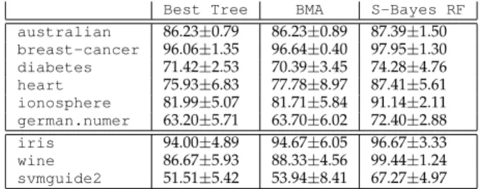
the label proportions of data points falling into each of the terminal nodes. The more label homogeneous is the terminal node, the more red or green or blue is the colour encoding. Note also that some of the terminal nodes are coloured black due to no data point falling into those particular nodes (this is a property unique to our usage of data independent prior on decision trees). However, these black internal nodes will not contribute to the importance weight of the tree as the associated terms in Equation (3) equal to 1. We gen-erate, in Figure 4, the operating curve of our method by varying the value ofβ from 1/N,2/N, . . . ,1. It is clear from the curves that Bayesian model averaging (the point wherem/N = 1) is suboptimal, except for small ‘iris’ dataset. For all datasets, effective sample size m = 5 seems to be sufficient. The experimental results for UCI datasets are summarised in Table 1. Inall but twodatasets (‘diabetes’ and ‘iris’), proposed S-Bayes RF method outperforms Bayesian decision trees (MCMC and SMC variants), sometimes by a large margin. We credit this to our usage of power likelihood that does not assume a single decision tree as a good hypothesis. This fact is corroborated in Table 2 where our weighted ensemble of trees always outperforms a single tree with the highest importance weight and BMA (whenβ= 1). Even though Bayesian random forest consists of randomly sampled trees, it is competitive to the random forest, where each tree is built with respect to some goodness criteria, in this case Gini impurity and entropy. However, Table 3 shows the drawback of our usage of power likelihood that it does not produce a well-calibrated predictive probabilities. We also assess the sensitivity of S-Bayes RF with the choice of number of trees and the splitting probabilityλ. The results for4representative datasets are visualised in Figure 5. For completeness, we also provide results of Bayesian Additive Regression Trees (BART) [13] using BayesTree package for R in Table 1–second to last column. We note that BART can be thought of as a Bayesian version of boosted decision trees. BayesTree package uses a probit link function for handling a binary classification problem. Our re-sults are consistent with previous studies [29] that found calibrated boosted trees were the best learn-ing algorithm on several considered binary learnlearn-ing

T ABLE 1: Accuracy acr oss 5 random repeats. D : number of dimensions and N : number of observations, equal fr om each class. kNN : k-near est neighbours ( k = 3 ), SVM : Supp ort vector machine with linear kernels, RF: Gini : Random for est learned with Gini impurity , RF: Ent. : Random for est learne d with information gain, MCMC : Markov chain monte carlo of Bayesian decision tr ee, SMC: pr. : Sequential monte carlo of Bayesian decision tr ee with prior pr oposal, SMC: ps. : Sequential monte carlo of Bayesian decision tr ee with posterior pr oposal, BART : a Bayesian version of boosted decision tr ees, and S-Bayes RF (Ours) : our Safe-Bayesian random for est. D N kNN SVM RF: Gini RF: Ent. MCMC SMC: prior SMC: post. BART S-Bayes RF australian 14 618 83.04 ± 2.53 86.23 ± 0.89 86.23 ± 2.29 86.08 ± 2.82 86.09 ± 0.61 86.23 ± 1.02 86.23 ± 0.51 87.68 ± 0.88 87.39 ± 1.50 breast-cancer 10 517 98.39 ± 1.25 98.54 ± 1.15 98.10 ± 1.42 98.10 ± 1.42 96.93 ± 1.58 96.35 ± 2.42 96.49 ± 1.66 98.39 ± 1.40 97.95 ± 1.30 diabetes 8 574 72.59 ± 1.32 75.32 ± 4.68 74.80 ± 2.61 74.15 ± 3.13 74.42 ± 2.08 71.68 ± 1.63 73.76 ± 2.08 76.75 ± 5.08 74.28 ± 4.76 heart 13 270 81.11 ± 5.54 85.18 ± 2.62 82.96 ± 4.01 83.33 ± 4.34 80.37 ± 6.23 79.63 ± 5.86 81.48 ± 5.71 85.56 ± 3.56 87.41 ± 5.61 ionosphere 34 270 81.99 ± 3.33 81.99 ± 6.59 90.85 ± 3.58 91.14 ± 3.41 89.43 ± 3.13 88.85 ± 2.93 89.71 ± 3.41 92.00 ± 3.28 91.14 ± 2.11 german.numer 24 680 63.80 ± 5.81 72.09 ± 4.04 69.29 ± 3.47 68.99 ± 3.18 63.80 ± 4.80 63.59 ± 6.25 64.10 ± 5.97 71.80 ± 3.78 72.40 ± 2.88 iris 4 60 95.99 ± 5.33 98.00 ± 2.98 96.67 ± 3.33 96.67 ± 3.33 96.67 ± 3.33 97.33 ± 2.78 95.99 ± 3.65 NA 96.67 ± 3.33 wine 13 178 97.22 ± 1.76 97.22 ± 3.40 98.33 ± 2.48 98.33 ± 2.48 95.56 ± 1.52 86.67 ± 9.89 94.44 ± 1.96 NA 99.44 ± 1.24 svmguide2 20 159 60.61 ± 2.71 69.70 ± 7.72 69.09 ± 4.97 67.87 ± 7.90 63.64 ± 9.34 55.15 ± 11.81 62.42 ± 5.90 NA 67.27 ± 4.97 (a) australian (b) breast-cancer (c) diabetes (d) heart (e) ionosphere (f) german.numer (g) iris (h) wine (i) svmguide2 Fig. 4: Operating curve of our Bayesian random for est based on the concept of power likelihood. Accuracy ± STE.. The curves ar e generated based on training data. The point wher e m/ N = 1 corr esponds to Bayesian model averaging (BMA).

australian 86.23±0.79 86.23±0.89 87.39±1.50 breast-cancer 96.06±1.35 96.64±0.40 97.95±1.30 diabetes 71.42±2.53 70.39±3.45 74.28±4.76 heart 75.93±6.83 77.78±8.97 87.41±5.61 ionosphere 81.99±5.07 81.71±5.84 91.14±2.11 german.numer 63.20±5.71 63.70±6.02 72.40±2.88 iris 94.00±4.89 94.67±6.05 96.67±3.33 wine 86.67±5.93 88.33±4.56 99.44±1.24 svmguide2 51.51±5.42 53.94±8.41 67.27±4.97

TABLE 3: Log predictive probabilities of Markov

chain Monte Carlo of Bayesian decision tree (MCMC) and weighted ensemble of trees with β = 5/N

(S-Bayes RF). Log probability±STD. As expected, in

all cases MCMC provides better calibrated probabili-ties than S-Bayes RF with power likelihood.

MCMC S-Bayes RF australian -0.3330±0.0249 -0.5409±0.0043 breast-cancer -0.0999±0.0336 -0.3009±0.0129 diabetes -0.5277±0.0149 -0.6260±0.0061 heart -0.4464±0.0560 -0.5879±0.0053 ionosphere -0.3150±0.0605 -0.6097±0.0095 german.numer -0.5885±0.0281 -0.6759±0.0023 iris -0.2616±0.1284 -0.5473±0.0608 wine -0.2475±0.0581 -0.6625±0.0275 svmguide2 -0.8702±0.0858 -1.0283±0.0133

problems but random forests are close second. In 3

datasets, BayesTree outperforms S-Bayes RF by more than0.4%while only in2datasets it was the opposite. The results on high dimensional image data are summarised in Table 4. Our results are once again consistent with [29] that found it surprising that random forest variants perform well even for high dimensional data. For this high dimensional data, we use effective sample size of one. Among trees and forest variants, our S-Bayes RF is the fastest to train, while MCMC based Bayesian decision tree is the most time consuming. We also run the random forest variant where a random subset of candidate features is used plus cut values are drawn at random for each candidate feature and the best of these randomly-generated thresholds is picked as the cut value [30], [31]. SMC with optimal proposals does not finish in three days. Our S-Bayes RF is implemented in Mat-lab while others are in Python. Although in general S-Bayes RF is fast, getting a precise runtime com-parison is not straightforward since implementation languages differ. In terms of accuracy performance, Bayesian decision trees perform comparably to the baseline kNN (13.20±2.41) for Israeli, and perform rather poorly to kNN (36.53±2.69) for AwA. The random forest and our Bayes random forestoutperform

ers, machine learning, computer vision, computer graphics, and medical image analysis. It typically works by averaging several predictions of randomly trained trees. In this paper, we show a conceptually radical approach to generate a random forest based on Bayesian statistics: random sampling of many trees from a prior distribution, and subsequently perform-ing a weighted ensemble.

Unlike other Bayesian models of decision trees which require computationally intensive Markov Chain Monte Carlo procedures, our framework utilises a data independent tree prior that facilitates offline tree generation. This prior allows us to sample a collection of decision trees even before looking at the data. Furthermore with the use of power likelihood, our method is able to explore space spanned by com-bining decision trees. This is in contrast to Bayesian decision trees where in the infinite data limit will put a mass to a single tree.

Our experimental results are encouraging, our S-Bayes RF outperforms S-Bayesian decision trees in term of speed and predictive performance, and is compet-itive with state-of-the-art random forest algorithms on both speed and accuracy. In the future, we are interested in exploring the possibility of adapting the power likelihood exponentβ as new data points arrive using for example the method of [19].

A

The authors would like to thank two anonymous reviewers for constructive comments and Sara Wade, Wray L. Buntine, Viktoriia Sharmanska, Sebastian Nowozin, and James Lloyd for discussions.

REFERENCES

[1] Leo Breiman, J. H. Friedman, R. A. Olshen, and C. J. Stone.

Classification and Regression Trees. Wadsworth, 1984.

[2] J. R. Quinlan. Induction of decision trees. Machine Learning, pages 81–106, 1986.

[3] Sebastian Nowozin. Improved information gain estimates for decision tree induction. InInternational Conference on Machine Learning (ICML), 2012.

[4] L. Breiman. Random forests. Technical Report TR567, UC Berkeley, 1999.

[5] Jamie Shotton, Andrew W. Fitzgibbon, Mat Cook, Toby Sharp, Mark Finocchio, Richard Moore, Alex Kipman, and Andrew Blake. Real-time human pose recognition in parts from single depth images. In Computer Vision and Pattern Recognition (CVPR), 2011.

[6] Gabriele Fanelli, Matthias Dantone, Juergen Gall, Andrea Fos-sati, and Luc Gool. Random forests for real time 3d face analysis. International Journal of Computer Vision, pages 1–22, 2012.

TABLE 4: Accuracy results of trees and forest variants on high dimensional images dataset across5 random repeats.C: number of categories.ExtraTrees: a random forest variant with random features and cut values.

D C N MCMC SMC: prior RF: Gini RF: Ent. ExtraTrees S-Bayes RF

Israeli-Images dataset

4,097 11 1,056 15.59±3.46 15.88±0.86 35.21±2.28 34.54±1.32 33.97±1.91 34.93±2.05 Animals with Attributes dataset

2,000 10 3,000 27.03±1.80 27.39±2.66 41.96±0.91 41.86±1.38 41.57±0.92 38.17±0.92

(a) australian (b) heart

(c)wine (d) svmguide2

Fig. 5:Sensitivity analysis of the performance of S-Bayes RF on test set with respect to the choices of splitting

probabilityλand number of trees #trees. We observe that in general S-Bayes RF is robust to the (λ,# trees)-parameter selection with the tendency of better accuracy performance with more trees andλclose to0.5.

[7] Antonio Criminisi, Jamie Shotton, and Ender Konukoglu. Decision forests: A unified framework for classification, re-gression, density estimation, manifold learning and semi-supervised learning.Foundations and Trends in Computer Graph-ics and Vision, 7(2-3):81–227, 2012.

[8] Tin Kam Ho. The random subspace method for constructing decision forests. IEEE Transactions on Pattern Analysis and Machine Intelligence, 20(8):832–844, 1998.

[9] Wray L. Buntine. Learning classification trees. Statistics and Computing, 2:63–73, 1992.

[10] Jonathan J. Oliver and David J. Hand. On pruning and

averaging decision trees. InInternational Conference on Machine Learning (ICML), 1995.

[11] Hugh Chipman, Edward I. George, and Robert E. Mcculloch. Bayesian cart model search. Journal of the American Statistical Association, pages 935–948, 1998.

[12] David G. T. Denison, Bani K. Mallick, and Adrian F. M. Smith. A bayesian cart algorithm. Biometrika, 85(2):363–377, 1998. [13] Hugh A. Chipman, Edward I. George, and Robert E.

Mc-Culloch. Bayesian ensemble learning. In Neural Information Processing Systems (NIPS), 2007.

[14] Balaji Lakshminarayanan, Daniel M. Roy, and Yee Whye Teh. Top-down particle filtering for bayesian decision trees. In

International Conference on Machine Learning (ICML), 2013. [15] T. P. Minka. Bayesian model averaging is not model

combi-nation. Technical report, MIT Media Lab., 2002.

[16] Hyun-Chul Kim and Zoubin Ghahramani. Bayesian classifier combination.Journal of Machine Learning Research - Proceedings Track, 22:619–627, 2012.

[17] Stephen Walker and Nils Lid Hjort. On bayesian consistency.

Journal of the Royal Statistical Society. Series B (Statistical Method-ology), 63(4):811–821, 2001.

[18] Isadora AntonianoVillalobos and Stephen G. Walker. Bayesian nonparametric inference for the power likelihood. Journal of Computational and Graphical Statistics, 2012.

[19] Peter Gr ¨unwald. The safe bayesian: Learning the learning rate via the mixability gap. InInternational Conference on Algorithmic Learning Theory (ALT), 2012.

[20] Tong Zhang. Learning bounds for a generalized family of bayesian posterior distributions. InNeural Information Process-ing Systems (NIPS), 2003.

[21] Wray L. Buntine.A Theory of Learning Classification Rules. PhD thesis, University of Technology Sydney, 1992.

[22] J. M. Hammersley and D. C. Handscomb.Monte Carlo methods. Methuen London, 1964.

[23] Joseph G. Ibrahim and Ming-Hui Chen. Power prior distribu-tions for regression models.Statistical Science, 15(1):pp. 46–60, 2000.

[24] N. Friel and A. N. Pettitt. Marginal likelihood estimation via power posteriors. Journal of the Royal Statistical Society: Series B (Statistical Methodology), 70(3):589–607, 2008.

[25] Robert Gramacy, Richard Samworth, and Ruth King. Impor-tance tempering.Statistics and Computing, 20(1):1–7, 2010. [26] Florent Perronnin, Jorge S´anchez, and Thomas Mensink.

Im-proving the fisher kernel for large-scale image classification. InEuropean Conference on Computer Vision (ECCV), 2010. [27] Herbert Bay, Andreas Ess, Tinne Tuytelaars, and Luc Van Gool.

Speeded-up robust features (surf). Computer Vision and Image Understanding, pages 346–359, 2008.

[28] F. Pedregosa et al. Scikit-learn: Machine learning in Python.

Journal of Machine Learning Research, 12:2825–2830, 2011. [29] R. Caruana, N. Karampatziakis, and A. Yessenalina. An

em-pirical evaluation of supervised learning in high dimensions. InInternational Conference on Machine Learning (ICML), 2008. [30] Adele Cutler and Guohua Zhao. Pert - perfect random tree

ensembles.Computing Science and Statistics, 2001.

[31] Pierre Geurts, Damien Ernst, and Louis Wehenkel. Extremely randomized trees.Machine Learning Journal, 63(1), 2006.