Cubic B-splines collocation method for solving a partial integro-differential equation with a weakly singular kernel

(1)

Cubic B-splines collocation method for solving a partial

integro-diﬀerential equation with a weakly singular kernel

Mohammad Gholamian

Department of Applied Mathematics, Faculty of Mathematical Sciences, Ferdowsi University of Mashhad, International Campus, Mashhad, Iran. E-mail: [email protected]

Jafar Saberi-Nadjafi∗

Ali Reza Soheili

Abstract In this paper, we apply a numerical scheme for the solution of a second order partial integro-differential equation with a weakly singular kernel. In the time direction, the backward Euler method time-stepping is used to approximate the differential term and the cubic B-splines is applied to the space discretization. Detailed discrete schemes, the convergence and the stability of the method is demonstrated. Next, the computational efficiency and accuracy of the method are examined by the numerical results.

Keywords. Cubic B-splines, Partial integro-diﬀerential equation, Backward Euler method.

2010 Mathematics Subject Classification. 65L05, 34K06, 34K28.

1. _Introduction

In this paper, we consider the following second order partial integro-diﬀerential equation with a weakly singular kernel

ut(x, t) =µuxx(x, t) +

∫ t

0

(t−s)−12_uxx₍_{x, s}₎_ds, _x∈_[_{a, b}_]_{, t}≥₀_, _(1.1)

whereµ≥0 and subject to the initial condition

u(x,0) =ν(x), (1.2)

with the boundary conditions

u(a, t) = 0, u(b, t) = 0, t≥0. (1.3)

Received: 18 September 2017 ; Accepted: 26 August 2018.

∗Corresponding author.

(2)

Such a problem can be appeared in mathematical modeling of some engineering and scientiﬁc systems that leads to a model by partial integro-diﬀerential equa-tions(PIDEs). The equations (1.1)-(1.3) can be appeared in the applications such as heat conduction in materials with memory [10, 22], population dynamics and vis-coelasticity [5,27].

Of course, some numerical methods have been applied for partial integro- differen-tial equations with weakly singular kernel. These methods are including finite-element methods [43]-[39], finite difference methods [33, 35], orthogonal spline collocation methods [1,8], spectral collocation methods [9,16], Galerkin methods [15] and quasi wavelet methods [17,42].

Because of the singularity of the kernel, inducing sharp transitions in the solution, there is a challenge in developing accurate numerical methods for solving the partial integro-differential equations. Thus, applying the collocation method by using the B-splines functions in handling the sharp transitions is caused by the singularities of the kernel is an effective way. Because there are two useful and important features of B-splines in numerical work. One is that the continuity conditions are inherent. Com-pared with other piecewise polynomial interpolation functions, the B-spline functions are the smoothest interpolation functions. Second feature is each B-spline function is only non-zero over a few mesh subintervals, i.e, B-splines have small local support property. Therefore, the resulting matrix is sparse. Because of having smoothness and capability to handle local phenomena, B-splines have been offered with special advantage. In the case it combined with the collocation, these advantages can signifi-cantly simplify the solution procedure of the differential equations. For example, the cubic B-splines have been used to compute the numerical solution of the Klein-Gordon equation [13]. The Regularized Long Wave RLW equation [28] can be solved by qua-dratic B-splines and the quantic B-splines has been used to build up the numerical solution of the Burgers equation in [30], the KdVB equation [44], the RLW equation [6], the Kuramoto-Sivashinsky equation [23] and cubic spline quasi-interpolation and multi-node higher order expansion have been used to solve the Burgers equation in [41]. Caglar [2, 3] used the B-splines to solve the boundary value problems. RLW equation can be solved by B-splines in [28, 29]. Most recently, the quantic B-spline collocation method is applied to obtain the numerical solution of fourth order partial integro-differential equations in [45].

The rest of the paper is organized as follows. In section 2, a detailed description about the cubic B-Splines is explained. In section 3, a numerical scheme for solving the problem (1.1)-(1.3) is discussed. The convergence analysis of the method is de-scribed in section 4. The stability analysis is carried out via Von-Neumann stability as given in section 5. In section 6, numerical experiments are tested to demonstrate the viability of the proposed method and this paper ends with a conclusion in section 7.

2. The cubic B-Splines

(3)

b−a

N , j = 0,1, . . . , N −1. The cubic B-splines Bj(x) forj =−1,0,· · ·, N+ 1 at the

knots are given as follows [24, 25]:

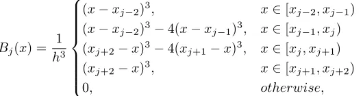
Bj(x) = 1

h3

              

(x−xj₋2)3, x∈[xj−2, xj−1) (x−xj₋2)3−4(x−xj₋1)3, x∈[xj₋1, xj)

(xj+2−x)3−4(xj+1−x)3, x∈[xj, xj+1) (xj+2−x)3, x∈[xj+1, xj+2)

0, otherwise,

(2.1)

where, {B₋1, B0, B1, . . . , BN−1, BN, BN+1} form a basis over the region a≤x≤b. Each cubic B-Spline covers four elements, so that each element is covered by four cubic B-splines. The values ofBj(x) and its ﬁrst and second derivatives are given as in Table 1.

Table 1. Coeﬃcients of cubic B-splines and its derivatives at knotsxj.

xj xj−2 xj−1 xj xj+1 xj+2

Bj(x) 0 1 4 1 0

B_j′(xj) 0 _h3 0 −_h3 0

B_j′′(xj) 0 _h62 −

12

h2

6

h2 0

Our numerical scheme for problem (1.1)-(1.3) using the collocation method with the cubic B-splines is to compute an approximate solutionUN(x, t) to the exact solution u(x, t) in the following form

UN(x, t) = N∑+1

j=−1

Cj(t)Bj(x), (2.2)

where, Bj(x) are the cubic B-splines in our proposed method, and Cj(t) are time

dependent quantities to be determined by the boundary conditions and collocation form of the partial integro-diﬀerential equation.

3. _{Numerical scheme}

In this section, we propose the numerical scheme for the solution of the problem Eqs. (1.1)-(1.3) in which the time derivative is dealt with the second order backward finite difference method and cubic B-splines are applied to the spacial derivative. First, we let the time level is denoted bytn=n∆t, n= 0,1, . . ., where ∆tis the time step. To apply the proposed method on Eq. (1.1) at time pointt =tn+1, the first expression in the left of Eq. (1.1) is approximated by

ut(x, tn+1)≈

un+1(x)−un(x)

∆t , a≤x≤b, n≥1. (3.1)

Therefore, for everyx∈[a, b], we have

un+1₍_x₎₋_un₍_x₎

∆t =µuxx+

∫ tn+1

0

(tn+1−s)−

1

(4)

For approximating the second expression in the right side of Eq. (3.2), we get

∫ tn+1

0

(tn+1−s)−

1

2_uxx₍_{x, s}₎_ds₌ ∫ tn+1

0

s−12_uxx₍_{x, tn}₊₁−_s₎_ds

=

n ∑

j=0

∫ tj+1

tj

s−12uxx(x, tn₊₁−s)ds

≈

n ∑

j=0

uxx(x, tn₋j+1)

∫ tj+1

tj

s−12_ds

= 2∆t12 n ∑

j=0

uxx(x, tn₋j+1)

[

(j+ 1)12 −_j12 ]

. (3.3)

By substituting Eq. (3.3) into Eq. (3.2) and rearranging, the Eq.(3.2) is become as follows

un+1(x)−µ∆tuxx(x, tn+1)−2∆t

3

2u_xx(x, t_n₊₁)

=un(x) + 2∆t32 n ∑

j=1

νjuxx(x, tn₋j+1), (3.4)

whereνj = (j+ 1)12 −j 1

2,j= 0,1, . . . , n.

Next, the spacial discretization of Eq. (3.4) is carried out by using Eq. (2.2) and the collocation method is implemented by identifying the collocation points as nodes. Therefore, fori= 0,1, . . . , N, yields

N_∑+1

j=−1

C_jn+1Bj(xi)−µ∆t N_∑+1

j=−1

C_jn+1B_j′′(xi)−2∆t32 N_∑+1

j=−1

C_jn+1B_j′′(xi)

=un_i + 2∆t32 n ∑

k=1

νk N∑+1

j=−1

C_jn−k+1B_j′′(xi), (3.5)

whereC_jn+1=Cj(tn+1),Uin+1is the approximate solution ofu(xi, tn+1) in Eq. (3.2) andB′′_j(xi) is the second order partial derivative with respect to the space variablex

ofBj at xi. Let

Di=un_i + 2∆t32 n ∑

k=1

νk N∑+1

j=−1

C_jn−k+1B_j′′(xi), i= 0,1, . . . , N. (3.6)

Therefore, we can rewrite Eq. (3.5) as follows

N_∑+1

j=−1

[

Bj(xi)−(µ∆t+ 2∆t32)B′′ j(xi)

]

C_jn+1=Di, i= 0,1, . . . , N. (3.7)

The system (3.7) consists ofN+1 linear equations withN+3 unknowns,C₋n+1₁ , C₀n+1, . . . , C_Nn+1₊₁. To compute the unique solution to this system, the parametersC₋n+1₁ and

(5)

expandu in terms of the cubic B-splines formula Eq. (2.2) atx0 =a andxN =b, yield

{

C₋1+ 4C0+C1= 0,

CN₋1+ 4CN +CN+1= 0.

(3.8)

By solving the Eq. (3.8), we get the values ofC₋1in terms ofC0andC1and similarly

CN+1 in terms ofCN₋1 andCN. Thus, the system (3.7) is reduced to a tridiagonal system ofN+ 1 linear equations andN+ 1 unknowns. For the sake of simpliﬁcation, the system (3.7) is denoted by the following matrix form

AC=D, (3.9)

where, the matricesA,C andDread as follow

A=

         

γ−4β 0 0 0 · · · 0

β γ β 0 · · · 0

0 β γ β . .. ...

..

. . .. . .. . .. . .. 0 0 · · · 0 β γ β

0 · · · 0 0 0 γ−4β           ,

C= [C₀n+1, C₁n+1, . . . , C_Nn+1]T, n= 0,1,2, . . . , D= [D0, D1, . . . , DN]T,

where,

β= 1−6∆t

h2 (µ+ 2∆t

1

2), γ= 4(1 + 3∆t

h2 (µ+ 2∆t

1

2)). (3.10)

Next, from the initial condition given in Eq. (1.2) and the collocation form (2.2), we deduce

u(x,0) =UN(x,0) = N∑+1

j=−1

C_j0Bj(x), x∈[a, b].

By partitioning [a, b] intoN + 1 points, namely x0, x1,· · · and xN, the initial vec-tor C0 _{= [}_C0

−1, C00,· · ·, CN0, C

0

N+1] can be obtained and next the initial numerical solutionU0

N = [UN(x0), UN(x1),· · ·, UN(xN)] results at the ﬁrst stept= 0, easily.

4. _{Convergence analysis}

(6)

4.1. The convergence in the spacial direction. LetUexactb (x) be the exact solu-tion of Eq. (1.1)-(1.3) andSb(x) be the cubic B-splines collocation approximation to

b

U(x). Then

b

S(x)≈Ubexact(x) = N∑+1

j=−1

b

Cj(t)Bj(x), (4.1)

whereCb= (Cb₋1,Cb0, . . . ,CbN+1).

Also, suppose that Se(x) be the computed cubic B-splines approximation to Sb(x), namely

e S(x) =

N∑+1

j=−1

e

Cj(t)Bj(x), (4.2)

where Ce = (Ce₋1,Ce0, . . . ,CNe +1). To estimate the error ∥ Uexactb (x)−Sb(x) ∥_∞, we must approximate the error∥ Uexactb (x)−Se(x)∥_∞ and ∥es(x)−bs(x)∥_∞ separately. According to Eq. (3.7), to compute Se(x) and Sb(x), we have to obtain the values of vectorsCb andCe from two systems of linear equations as follows

ACb =Db, (4.3)

and

ACe =De. (4.4)

By subtracting Eqs. (4.3) and (4.4), we obtain

A(Ce −Cb) =De −Db. (4.5)

Furthermore,Ais a strictly diagonally dominant matrix. Thus, it is nonsingular and we have

e

C−Cb =A−1(De −D)b . (4.6)

Taking inﬁnity norm from both sides of Eq. (4.6), we obtain

∥Ce −Cb ∥_∞≤∥A−1∥_∞∥De −Db ∥_∞. (4.7) Now consider that λi(0 ≤i ≤ N) is the summation of the ith row of matrix A =

[aij](N+1)(N+1). Therefore, we get

λ0=

N ∑

j=0

a0j=γ−4β, (4.8)

λi= N ∑

j=0

aij =γ+ 2β, i= 1, . . . , N−1, (4.9)

λN = N ∑

j=0

(7)

Due to the theory of matrices

N ∑

i=0

a−_ki1λi= 1, k= 0,1, . . . , N, (4.11)

wherea−_ki1 are the entries ofA−1_{. Thus,}

∥A−1∥_∞=

N ∑

i=0

|a−_ki1| ≤ 1

λ, (4.12)

whereλ= min0_≤i_≤Nλi = min{γ−4β, γ+ 2β}= min{η,6} andη= 36∆_h2t(µ+ 2∆t 1 2).

Substituting Eq. (4.12) into Eq. (4.7) we can ﬁnd

∥Ce −Cb ∥_∞≤ 1

λ∥De −Db ∥∞. (4.13)

For computing the upper bound of ∥ De −Db ∥_∞, from Eq. (3.6) for all values of 0≤i≤N, we conclude

|Dei−Dbi| ≤ |Uei−Ubi|

+12∆t

3 2 h2

n ∑

k=1

|νk|(|Ce_in₋−₁k+1−Cb_in₋−₁k+1|

+ 2|Ce_in−k+1−Cb_in−k+1|+|Ce_in₊₁−k+1−Cb_in₊₁−k+1|). (4.14)

Now, we need to recall the following theorem.

Theorem 4.1. Iff(x)∈c4[a, b],|f(4)(x)| ≤L,∀x∈[a, b] and

∆ ={a=x0< x1<· · ·< xN =b}

be the equally spaced partition of[a, b]with step size hand s(x) is the unique spline function interpolatef(x)at knots x0, x1, . . . , xN, then there exits a constantλj such that,

||f(j)−s(j)||_∞≤λjLh4−j, j= 0,1,2,3.

Proof. See [7]-[11].

According to the above theorem, we have

|Uei−Ubi|=|Se(xi)−Sb(xi)| ≤λ0Lh4. (4.15) In addition,{νk}n_k₌₁ is a sequence of positive terms descending andνk ≤1 for 1 ≤

k≤n. Thus, from Eq. (4.15) we can rewrite Eq. (4.14) as follows

||De −Db||_∞≤λ0Lh4+ 12∆t32

h2

n ∑

k=1

mk, (4.16)

where

(|Ce_in₋−₁k+1−Cb_in₋−₁k+1|+ 2|Ce_in−k+1−Cb_in−k+1|+|Ce_in₊₁−k+1−Cb_in₊₁−k+1|)≤mk.

By assuming∑n_k₌₁mk=Mn andλ0Lh4+12∆t

3 2

h2 Mn=Kn, we get

(8)

Using Eq. (4.17), from Eq. (4.13) we come up with

∥Ce −Cb ∥_∞≤Kh2, (4.18)

whereKh2₌ 1

λKn= max(

1 6,

1

η)Kn.

To proceed the rest, we note the following theorem.

Theorem 4.2. The B-splines{B₋1, B0, B1, . . . , BN₋1, BN, BN+1}satisfy the

follow-ing inequality

|

N_∑+1

j=−1

Bj(x)| ≤1, 0≤x≤1. (4.19)

Proof. See [26].

Now, by subtracting (4.2) from Eq. (4.1), we have

e

S(x)−Sb(x) =

N∑+1

j=−1

(Cej−Cbj)Bj(x). (4.20)

Using the above theorem and taking norm from (4.20), we obtain

∥Se(x)−Sb(x)∥_∞=

N∑+1

j=−1

(Cej−Cbj)Bj(x)

∞

≤ N_∑+1

j=−1

Bj(x)∥Cje −Cjb ∥_∞

≤Kh2. (4.21)

Theorem 4.3. Let Ub(x) be the exact solution of Eq. (1.1)-(1.3) and Sb(x) be the B-spline collocation approximation to Ub(x), then the method has second order con-vergence and

∥Ub(x)−Sb(x)∥_∞≤ωh2, (4.22)

whereω=λ0Lh2+K is ﬁnite constant.

Proof. From Theorem 4.2 we have

∥Ub(x)−Se(x)∥_∞≤λ0Lh4. (4.23)

Therefore, from Eqs. (4.21) and (4.23) we get

∥Ub(x)−Sb(x)∥_∞≤∥Ub(x)−Se(x)∥_∞+∥Se(x)−Sb(x)∥_∞ ≤λ0Lh4+Kh2

=ωh2, (4.24)

(9)

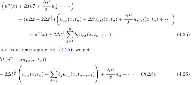
4.2. The convergence in the temporal direction. To get the estimate the con-vergence in temporal direction, we applied Taylor expansion to Eq. (3.4). Therefore,

(

un(x) + ∆tun_t +∆t 2

2! u

n tt+· · ·

)

−(µ∆t+ 2∆t32) (

uxx(x, tn) + ∆tuxxt(x, tn) +

∆t2

2! uxxtt(x, tn) +· · ·

)

=un(x) + 2∆t32 n ∑

j=1

bjuxx(x, tn−j+1), (4.25)

and from rearranging Eq. (4.25), we get

∆t(un_t −µuxx(x, tn))

−2∆t32 

uxx(x, tn) +

n ∑

j=1

bjuxx(x, tn₋j+1)

 +∆t

2

2! u

n

tt+· · ·=O(∆t). (4.26)

Finally, if we letu(x, t) is the exact solution of the Eq. (1.1)-(1.3) anduN₍_{x, t}_{) is the}

numerical approximation to this solution by applying the numerical method, we will have

∥u(x, t)−uN(x, t)∥≤ρ(k+h2), (4.27)

whereρis ﬁnite constant.

5. _{The stability of the method}

By Von-Neumann stability, we prove the stability of the proposed method. Using Table 1 and Eq. (3.7), for anyxi, i= 0,1, . . . , N, we get

βC_in₋+1₁ +γC_in+1+βC_in₊₁+1=Di, (5.1)

where

Di= (Cin₋1+ 4Cin+Cin+1) + 12∆t32

h2

n ∑

l=1

νl(C_in₋−₁l+1−2C_in−l+1+C_in₊₁−l+1).

We suppose that the solution of Eq. (3.7) is presented as

C_in =ξnekiηh,

whereξ represents the time dependence of the solution, the exponential function shows the spatial dependence such thatηhrepresents the position along the grid and

kis√−1. By substitutingCn

i into Eq. (5.1), we have

pξn+1ekiηh=qξnekiηh+12∆t

3 2 h2

n ∑

l=1

(10)

where     

p=β(ekηh+e−kηh) +γ, q=ekηh₊_e−kηh_{+ 4}_,

r=ekηh+e−kηh−2.

(5.3)

Furthermore, by substituting the values ofγ and β from Eq. (3.10) into Eq. (5.3) and usingekηh₊_e−kηh_{= 2}_cosηh_{, Eq. (}_5.3_{) becomes as follows:}

    

p= 2(1−6∆_h2t(µ+ 2∆t 1

2))cosηh+ 4(1 +3∆t

h2 (µ+ 2∆t 1 2)), q= 2cosηh+ 4,

r= 2cosηh−2.

(5.4)

Now, dividing both sides of Eq. (5.2) byP ξeikηh _{and after rearranging the results}

equation, we have

ξn−(q

p+

12∆t32 h2

r pν1)ξ

n−1₋12∆t

3 2 h2 r p n ∑ l=2

νlξn−l= 0. (5.5)

We choose

  

a1=−(q_p+12∆t

3 2 h2

r pν1),

al=−12∆t

3 2 h2

r

pνl, l= 2, . . . , n.

(5.6)

Using Eq. (5.6), Eq. (5.5) becomes as follows

ξn+a1ξn−1+a2ξn−2+· · ·+an₋1ξ+an= 0. (5.7)

It is easy to see that in Eq. (5.4)q >0 andr >0(h̸= 0). Ifβ≥0, we havep >0. In the rest of the procedure, we also need to use the following theorem:

Theorem 5.1. For all values of rootsxi of an arbitrary polynomial as

P(x) =a0xn+a1xn−1+· · ·+an,

we have

|ξi| ≤max{1, n ∑

j=1 |aj

a0

|}. (5.8)

Proof. For the proof see [32].

For the stability, it should be proved that all rootsξiof the Eq. (5.7) satisfy|ξi| ≤1. According to the Theorem 5.1, we have

n ∑

j=1 |aj

a0| = q+

12∆t32 h2 r

∑n j=1νj

p =

q+12∆t32

h2 r[(n+ 1) 1 2 −1]

p , (5.9)

where

n ∑

j=1

νj= n ∑

j=1

[(j+ 1)12 −j 1

2] = (n+ 1) 1

(11)

Now, by using Theorem 5.1, from Eq. (5.9) we obtain

q+12∆t

3 2

h2 r[(n+ 1)

1

2 −1]< p. (5.11)

By using Eq. (5.4), we get

cosηh < γh

2_{+ 24∆}_t3

2[(n+ 1) 1 2 −1]

12∆t(3∆t12 +µ)

. (5.12)

Therefore, for conditional stability of the method, Eq. (5.12) must be valid.

6. Numerical experiments

In this section, we present some numerical results to demonstrate the eﬃciency and accuracy of the proposed method. All calculations are run with Matlab R2014a software on a Pentium PC Laptop with Core i3-350M Processor 2.26 GHz of CPU and 4G RAM. We have solved the problem based on a variety of temporal and spatial divisions. In numerical experiments, we have used the variablesM andNfor temporal and spatial divisions, respectively.

Furthermore, because of conditionally stability, we have applied the stability condition for temporal and spatial divisions and obtained the Errors of computations inL2and

L_∞error norms as follows

L2=∥uexact−unum∥2=

(_N ∑

i=0

|uexact_i −unum_i |2 )1/2

,

L_∞=∥uexact−unum∥_∞= max 0≤i≤N |u

exact i −u

num i |,

Example 6.1.Consider the following weakly singular partial integro-diﬀerential equa-tion in case ofµ= 0in Eq. (1.1) [19,34].

ut(x, t) = ∫ t

0

(t−s)−12u_xx(x, s)ds, x∈[0,1], t≥0,

with the boundary and initial conditions

u(0, t) =u(1, t) = 0, 0≤t≤1,

u(x,0) = sin(πx), 0≤x≤1.

The exact solution isu(x, t) =M(π52t 3

2) sin(πx), whereM denotes the seriesM(z) = ∑+_∞

0 (−1)

n_Γ(3

2n+ 1)− 1_zn_.

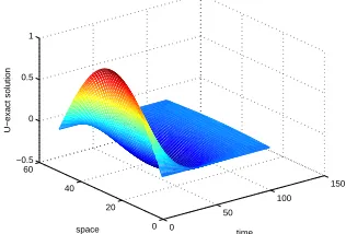
We have solved the problem based on a variety of temporal and spatial divisions and applied the stability condition for temporal and spatial divisions. The errors of computations are obtained in L2 and L_∞. The numerical and exact solutions are shown for a case of divisions asM = 50 andN= 100 in Figures 1 and 2.

(12)

Figure 1. The numerical solution forM = 100 andN = 50.

0 50

100 150

0 20 40 60 −0.5 0 0.5 1

time space

U−numerical solution

Figure 2. The exact solution forM = 100 andN = 50.

0 50

100 150

0 20 40 60 −0.5 0 0.5 1

time space

U−exact solution

Figure 3. The error forM = 100 andN = 50.

0 50

100 150

0 20 40 600 0.01 0.02 0.03 0.04 0.05

time space

Error

7. _Conclusion

(13)

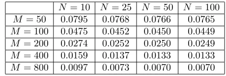
Table 2. TheL∞ error norm for some cases of divisions ofN andM.

N= 10 N = 25 N = 50 N = 100

M = 50 0.0795 0.0768 0.0766 0.0765

M = 100 0.0475 0.0452 0.0450 0.0449

M = 200 0.0274 0.0252 0.0250 0.0249

M = 400 0.0159 0.0137 0.0133 0.0133

M = 800 0.0097 0.0073 0.0070 0.0070

results have also demonstrated that the proposed computational method is eﬃcient for these type of problems.

References

[1] B. Bialecki and G. Fairweather, Orthogonal spline collocation methods for partial diﬀerential equations, J. Comput. Appl. Math.,128(2001), 55–82.

[2] N. Caglar and H. Caglar,B-spline method for solving linear system of second-order boundary value problems, Comput. Math. Appl.,57(2009), 757–762.

[3] N. Caglar and H. Caglar,B-spline solution of singular boundary value problems, Appl. Math. Comput.,182(2006), 1509–1513.

[4] C. Chen, V. Thom´ee, and L. Wahlbin,Finite element approximation of a parabolic integro-diﬀerential equation with a weakly singular kernel, Math. Comput.,58(1992), 602–587. [5] R. M. Christensen and L. B. Freund,Theory of viscoelasticity. J. Appl. Mech.,38(1971), 720–

722.

[6] I. Dag, B. Saka, and D. Irk,Galerkin method for the numerical solution of the RLW equation using quintic B-splines, Comput. Appl. Math.,190(2006), 532–547.

[7] C. De Boor,On the convergence of odd degree spline interpolation, Journal of Approx. Theory, 1(1968), 452–463.

[8] G. Fairweather,Spline collocation methods for a class of hyperbolic partial integro-diﬀerential equations, SIAM J. Numer. Anal.,28(1994), 444–460.

[9] F. Fakhar-Izadi and M. Dehghan,The spectral methods for parabolic Volterra integro-diﬀerential equations, J. Comput. Math.,235(2011), 4032–4046.

[10] M. E. Gurtin and A. C. Pipkin,A general theory of heat conduction with ﬁnite wave speeds, Arch. Ration. Mech. An.,31(1968), 113–126.

[11] C. A. Hall,On error bounds for spline interpolation, J. Approximation Theory.,1(1968), 209– 218.

[12] Y. Huang,Time discretization scheme for an integro-diﬀerential equation of parabolic type, J. Comput. Math.,12(1994), 259–263.

[13] M. Lakestani and M. Dehghan, Collocation and finite difference-collocation methods for the solution of nonlinear Klein-Gordon equation, Comput. Phys. Commun.,181(2010), 1392–1401. [14] S. Larsson, V. Thomée, and L. Wahlbin, Numerical solution of parabolic integro-differential

equations by the discontinuous Galerkin method, Math. Comput.,67(1998), 45–71.

[15] T. Lin, Y. Lin, M. Rao, and S. Zhang,Petrov-Galerkin methods for linear Volterra integro-diﬀerential equations, SIAM J. Numer. Anal.,38(2001), 937–963.

[16] Y. Lin and C. Xu,Finite diﬀerence/spectral approximations for the time-fractional diﬀusion equation, J. Comput. Phys.,225(2007), 1533–1552.

[17] W. Long, D. Xu, and X. Zeng, Quasi wavelet based numerical method for a class of partial integro-diﬀerential equation, Appl. Math.Comput.,218(2012), 11842–11850.

[18] C. Lubich,Discretized fractional calculus, SIAM J. Math. Anal.,17(1986), 704–719.

(14)

[20] W. McLean, V. Thom´ee, and L. Wahlbin,Discretization with variable time steps of an evolution equation with a positive-type memory term, J. Comput. Appl. Math.,69(1996), 49–69. [21] W. McLean and V. Thom´ee,Numerical solution of an evolution equation with a positive-type

memory term, J. Aust. Math. Soc.,35(1993), 23–70.

[22] R. K. Miller,An integro diﬀerential equation for rigid heat conductors with memory, J. Math. Anal. Appl.,66(1978), 313–332.

[23] R. C. Mittal and G. Arora,Quintic B-spline collocation method for numerical solution of the Kuramoto-Sivashinsky equation, Commun. Nonlinear Sci. Numer. Simul.,15(2010), 2798–2808. [24] R. C. Mittal and G. Arora,Numerical solution of the coupled viscous Burgers’ equation,

Com-mun. Nonlinear Sci. Numer. Simul.,16(2011), 1304–1313.

[25] R. C. Mittal and R. K. Jain,Cubic B-spline collocation method for solving nonlinear parabolic partial diﬀerential equations with Neumann boundary conditions, Commun. Nonlinear Sci. Nu-mer. Simul.,17(2012), 4616–4625.

[26] P. M. Prenter,Spline and Variational Methods, Wiley, New York, 1975. [27] M. Renardy,Mathematical analysis of viscoelastic ﬂows, Siam., 2000.

[28] B. Saka and I. Dag,A numerical solution of the RLW equation by Galerkin method using quartic B-splines, Commun. Numer. Methods Eng.,24(2008), 1339–1361.

[29] B. Saka, I. Dag, and D. Irk,Quintic B-spline collocation method for numerical solution of the RLW equation, J. ANZIAM.,49(2008), 389–410.

[30] B. Sepehrian and M. Lashani,A numerical solution of the Burgers equation using quintic B-splines, In Proceedings of the World Congress on Engineering, London, UK, July 2 - 4, (2008). [31] I. Sloan and V. Thom´ee,Time discretization of an integro-diﬀerential equation of parabolic

type, SIAM J. Numer. Anal.,23(5) (1986), 1052–1061.

[32] J. Stoer and R. Bulirsch,Introduction to Numerical Analysis, Second edition, Springer-Verlag, New York, 1991.

[33] Z. Sun and X. Wu,A fully discrete diﬀerence scheme for a diﬀusion-wave system, Appl. Numer. Math.,56(2006), 193–209.

[34] T. Tang,A finite difference scheme for partial integro-differential equations with a weakly sin-gular kernel, Appl. Numer. Math.,11(1993), 309–319.

[35] T. Tang,Superconvergence of numerical solutions to weakly singular Volterra integro-diﬀerential equations, Numer. Math.,61(1992), 373–382.

[36] D. Xu, Non-smooth initial data error estimates with the weight norms for the linear ﬁnite element method of parabolic partial diﬀerential equations, Appl. Math. Comput., 54 (1993), 1-24.

[37] D. Xu,On the discretization in time for a parabolic integro-diﬀerential equation with a weakly singular kernel I: nonsmooth initial data, Appl. Math.Comput.,57(1993), 1–27.

[38] D. Xu,On the discretization in time for a parabolic integro-diﬀerential equation with a weakly singular kernel II: smooth initial data, Appl. Math. Comput.,57(1993), 29–60.

[39] D. Xu,The global behavior of time discretization for an abstract Volterra equation in Hilbert space, Calcolo.,34(1997), 71–104.

[40] D. Xu,The long-time global behavior of time discretization for fractional order Volterra equa-tions, Calcolo.,35(1998), 93–116.

[41] M. Xu, R. Wang, and J. Zhang,A novel numerical scheme for solving Burgers’ equation, Appl. Math. Comput.,217(2011), 4473–4482.

[42] X. Yang, D. Xu, and H. Zhang,Crank-Nicolson/quasi-wavelets method for solving fourth order partial integro-diﬀerential equation with a weakly singular kernel, J. Comput. Phys.,234(2013), 317–329.

[43] E. Yanik and G. Fairweather, Finite element methods for parabolic and hyperbolic partial integro-diﬀerential equations, Non-Linear Anal.,12(1988), 809–821.

[44] S. I. Zaki,A quintic B-spline ﬁnite elements scheme for the KdVB equation, Comput. Methods Appl. Eng.,188(2000), 121–134.