A No-Arbitrage Approach to Range-Based Estimation of Return Covariances and Correlations

(1)

Financial

Institutions

Center

A No-Arbitrage Approach to

Range-Based Estimation of Return

Covariances and Correlations

by

Michael W. Brandt Francis X. Diebold 03-15

(2)

The Wharton Financial Institutions Center

The Wharton Financial Institutions Center provides a multi-disciplinary research approach to the problems and opportunities facing the financial services industry in its search for competitive excellence. The Center's research focuses on the issues related to managing risk at the firm level as well as ways to improve productivity and performance.

The Center fosters the development of a community of faculty, visiting scholars and Ph.D. candidates whose research interests complement and support the mission of the Center. The Center works closely with industry executives and practitioners to ensure that its research is informed by the operating realities and competitive demands facing industry participants as they pursue competitive excellence.

Copies of the working papers summarized here are available from the Center. If you would like to learn more about the Center or become a member of our research community, please let us know of your interest.

Franklin Allen Richard J. Herring

Co-Director Co-Director

The Working Paper Series is made possible by a generous grant from the Alfred P. Sloan Foundation

(3)

A No-Arbitrage Approach to Range-Based Estimation

of Return Covariances and Correlations

*

Michael W. Brandta and Francis X. Dieboldb

Duke University University of Pennsylvania and NBER and NBER

First Draft: September 2001 This Draft: April 2003

Abstract: We extend range-based volatility estimation to the multivariate case. In particular, we propose a range-based covariance estimator motivated by a key financial economic consideration, the absence of arbitrage, in addition to statistical considerations. We show that this estimator is highly efficient yet robust to market microstructure noise arising from bid-ask bounce and asynchronous trading.

Keywords: Range-based estimation, volatility, covariance, correlation, absence of arbitrage, exchange rates, stock returns, bond returns, bid-ask bounce, asynchronous trading

_______________

*

This work was supported by the National Science Foundation, the Wharton Financial Institutions Center, and the Rodney L. White Center for Financial Research at the Wharton

School. We thank Al Madansky and an anonymous referee for insightful and forceful comments. We also thank Tim Bollerslev, Celso Brunetti, Rob Engle, Joel Hasbrouck, Peter Lildolt, Jeff Russell, and Neil Shephard, as well as seminar participants at the University of Pennsylvania and at CIRANO for insightful discussions and comments. Clara Vega provided outstanding research assistance.

a c

Department of Finance, Duke University, and NBER [email protected]

b

c_{Departments of Economics, Finance and Statistics, University of Pennsylvania, and NBER}

[email protected]

(4)

1 _{The relevant literature includes Garman and Klass (1980), Parkinson (1980), Beckers (1983), Ball and Torous} (1984), Rogers and Satchell (1991), Kunitomo (1992), and Yang and Zhang (2000).

1. Introduction

The price range, defined as the difference between the highest and lowest log asset prices over a fixed sampling interval (for concreteness, we focus on a one-day interval), has a long, colorful, and distinguished history of use as a volatility estimator.1_{As emphasized most recently}

by Alizadeh, Brandt and Diebold (2002), the range is a highly efficient volatility proxy, distilling volatility information from the entire intraday price path, in contrast to volatility proxies based on the daily return, such as the daily squared return, which use only the opening and closing prices. Moreover, data on the range are widely available for individual stocks and for exchange-traded futures contracts (including currencies, Treasury securities, and stock indices), not only presently but also, in many cases, over long historical spans. In fact, the range has been reported for many decades in business newspapers through so-called “candlestick plots,” showing the daily high, low, and close.

Despite these appealing properties of the range, one cannot help but notice a large and striking gap in the range-based volatility estimation literature: it is entirely univariate. That is, although based variance estimation has been extensively discussed and refined, range-based covariance estimation remains uncharted territory. The reason is that it is not at all obvious how to construct an appropriate range-based covariance estimator. Hence the range would seem to join the ranks of other famously obvious and intuitive univariate statistics, such as the median, that have no similarly obvious or intuitive multivariate generalization.

The apparent failure of range-based volatility estimation to generalize to the multivariate case is particularly unfortunate because financial economics is intimately concerned with

(5)

(1) multivariate interactions. Consider, for example, three pillars of modern finance: asset pricing, asset allocation, and risk management. Asset prices depend on covariance with the market and perhaps other risk factors. Similarly, optimal portfolio shares depend on the variances and

covariances of asset returns, as does portfolio vale at risk.

We attempt to remedy the situation by proposing a simple and intuitive range-based covariance estimator. Our approach is not merely statistical; rather, it relies appealingly on a key financial economic consideration, the absence of arbitrage. In particular, we use no-arbitrage conditions to express covariances in terms of variances, which may then be estimated by standard range-based methods.

2. Range-Based Variance and Covariance Estimation

Before considering the range-based estimation of covariances, we must set the stage by considering certain aspects of univariate volatility estimation. Consider a univariate stochastic volatility diffusion for the log of an asset price p_t with instantaneous volatility F_t. Suppose we sample this process discretely at m regular times throughout the day, which lasts from time t to

t+1, to obtain the intraday returns , for . Under conditions given in Andersen, Bollerslev and Diebold (2003), the variance of the discrete-time returns over the one-day interval conditional on the sample path is

The integrated volatility thus provides a canonical and natural measure of return volatility, and it features prominently in the financial economics literature (e.g., Hull and White, 1987). Because the integrated volatility is inherently unobservable, several estimators have been proposed, including estimators based on daily returns (e.g., daily squared or absolute returns),

(6)

(3) (2) high-frequency intraday returns (e.g., the “realized volatility” of Andersen, Bollerslev, Diebold and Labys, 2003), and the daily range. In particular, Parkinson’s (1980) celebrated range-based estimator of the daily integrated variance is given by

The univariate range-based volatility estimator has several appealing properties. First, it is of course trivial to compute. Second it is unbiased and highly efficient relative to competitors such as the squared or absolute daily return (Andersen and Bollerslev, 1998). Finally, it is robust to certain types of microstructure noise, such as bid-ask bounce (Alizadeh, Brandt and Diebold, 2002).

Now consider the multivariate case. In parallel with our univariate discussion, consider a stochastic volatility diffusion for a vector of log asset prices with diffusion matrix , whose ij-th element we denote . Then, again under conditions given in Andersen, Bollerslev and Diebold (2003), the one-day conditional covariance of the discrete-time returns on assets I and j is just the integrated instantaneous covariance,

The attractive blend of convenience, efficiency and robustness achieved by the range-based estimator in the univariate estimation of integrated volatility (1) makes one hungry for extension to a range-based estimator of the integrated covariance (3) in the multivariate case. We now proceed to do so. The basic idea is very simple, and the implementation varies slightly

(7)

(4)

(5)

(6)

(7) in turn.

First consider foreign exchange. In foreign exchange markets, absence of triangular arbitrage implies a deterministic relationship between any pair of dollar rates and the

corresponding cross rate. Consider two dollar exchange rates, denoted A/$ and B/$. Then, in the absence of triangular arbitrage, the cross-rate is

and hence the continuously compounded A/B return is . Taking variances gives

and solving for the covariance yields

This suggests a natural covariance estimator,

where can in principle be any return variance estimator. Given the desirable properties of range-based volatility estimation discussed above, we advocate the use of Parkinson’s (1980) range-based estimator in equation (2). We then assemble the estimated variance-covariance matrix as

(8)

(9)

(10) In higher dimensional cases, we proceed in analogous fashion, estimating each pairwise

covariance as above, and then assembling the results into an estimated covariance matrix. Now consider fixed income markets, in which the absence of arbitrage implies a deterministic relationship among any two zero-coupon bond prices and the corresponding

forward contract. Specifically, consider two bonds with maturities T₁ and T₂ and prices P(T₁) and

P(T₂), with T₁<T₂. The price of a forward contract between times T₁ and T₂ is

Taking logs gives and then taking first differences gives and finally taking variances gives

Hence we can form the covariance estimator,

and assemble the estimated variance-covariance matrix precisely as in the foreign exchange case. Finally, consider equities. The return on a two-equity portfolio with shares and ,

(9)

(11)

(12) denoted , has a variance of

which suggests the covariance estimator,

This method of estimating the covariance via the range of the two-asset portfolio return is

generally applicable to any two assets – not just equities – if data on the portfolio return range are available.

3. Discussion

Our no-arbitrage approach to range-based covariance estimation is widely applicable in the foreign exchange context because daily ranges of all legs of many currency triangles are available. For example, Datastream provides as much as 40 years of historical data on the daily high, low, and closing prices of 37 British pound denominated currencies and 14 Swiss franc denominated currencies. The International Monetary Market, a subsidy of the Chicago

Mercantile Exchange, recently introduced futures and options contracts on Euro/British pound, Euro/Swiss franc, and Euro/Japanese yen cross rates. Finally, the New York Board of Trade offers futures contracts on 14 cross-currencies, including seven Euro denominated contracts.

We hasten to add, however, that the practical applicability of our approach in other contexts is far more limited. For fixed income, our approach is only directly applicable to select maturities for which liquid bonds are aligned with liquid forward or futures contracts, such as the three- and six-month Eurodollar deposits and the three-month Eurodollar futures. For equities, our approach will rarely be applicable, because historical data on the range of two-asset

(10)

2 _{Some notable exceptions are the TSE 100, TSE 200, and TSE 300 indices of the Toronto stock}

exchange and the ASX 100, ASX 200, and ASX 300 indices of the Australian stock exchange.

3 _{Other ways to guarantee positive definiteness include the shrinkage approach of Ledoit and Wolf}

(2001) or the perturbation methods of Gill, Murray and Wright (1981) and Schnabel and Eskow (1999).

portfolios are typically not available.2

Thus far we have said little about the theoretical properties of the range-based covariance estimator. One obvious point is that the covariance estimator is unbiased under the same

conditions that deliver unbiasedness of Parkinson’s (1980) variance estimator because it is a linear combination of variances. Conversion to correlation, however, will introduce bias due to the nonlinearity of the transformation.

A similarly obvious and related point is that is in general not guaranteed to be positive definite. In our experience, however, positive definiteness is rarely violated in practice. If desired, positive definiteness can be imposed by estimating the Cholesky factor P of , rather than itself, where P is the unique lower-triangular matrix defined by . Note that the elements of P are functions of the elements of . Hence we insert our range-based estimators of the relevant variances and covariances into P (computed analytically) to obtain an estimator of the Cholesky factor and then form the estimator of the covariance matrix. Because the estimated Cholesky factor will be complex when is not positive definite, we define as the conjugate transpose, which guarantees that is real.3

Ultimately, however, the interesting questions for financial economists center not on the theoretical properties of range-based covariance and correlation estimates under abstract

conditions surely violated in practice, but rather on their performance in realistic situations involving small samples, discrete sampling, and market microstructure noise. As we argued

(11)

(13) above, we have reason to suspect good performance of the range-based approach, both because of its high efficiency due to the use of the information in the intraday sample path, and because of its robustness to microstructure noise. We now turn to a brief Monte Carlo analysis designed to illuminate precisely those issues.

4. Monte Carlo Exploration

We initially ignore market microstructure issues. We assume that two

dollar-denominated exchange rates and evolve as driftless diffusions with annualized volatilities F of 15 percent, a covariance of 0.9, and hence a correlation D of 0.4. We further assume that at

each instant the cross-rate is determined by the absence of triangular arbitrage as the ratio of the two dollar rates. Starting at , we simulate 24 hours worth of regularly spaced intraday log price observations using:

where , are standard normal innovations with correlation D, and there are 250 trading days per year. We consider sampling frequencies m ranging from m=18 (one observation every 1 hour and 20 minutes) to m=1440 (one observation every minute) and use the resulting data to compute the daily range and intraday returns. We then construct three estimates of the volatilities, covariance, and correlation of the two dollar rates. Specifically, we construct range-based covariance matrix estimates using Parkinson’s variance estimator (2) and equation (7), and, for comparison, we compute the realized covariance matrix using two different approaches. First, in parallel fashion to the range-based estimator, we use the three realized variances

(12)

4_Since _and _{follow the same stochastic process, we analyze only the volatility estimates for} _.

Second, we compute the realized covariance directly using the cross-products of intraday returns. We repeat this procedure 10,000 times and report the means, standard deviations, and root mean squared errors of the resulting sampling distributions in Table 1.

The results for the volatilities are familiar from Alizadeh, Brandt, and Diebold (2002).4

The range-based estimates are downward biased because the range of the discretely sampled process is strictly less than the range of the underlying diffusion. The magnitude of the bias decreases as the sampling frequency increases. But, even in the limit as , the range is still only a noisy volatility proxy, which means that the standard deviation and RMSE of the range-based volatility estimator settle down to non-zero values. The realized volatility behaves quite differently because it converges not only in expectation but also in realization to the true

volatility. The more frequently the underlying diffusion is sampled, the more precise the realized volatility gets, until, in the limit, the standard deviation and RMSE of the estimator are zero.

The results for the range-based covariance estimates follow from the properties of the range-based volatility estimates. The estimator

involves three volatility estimates, each of which is downward biased by an amount that depends on the level of volatility (the higher the volatility the more likely that the true extremes are far from the observed extremes). Because the variance of is less than the variance of and due to the positive covariance, the

covariance estimates are also downward biased because the downward bias of

dominates the upward bias of . As with the volatility estimates, the bias vanishes as we increase the sampling frequency, and the standard deviation and RMSE stabilize. The realized covariances, computed either through the no-arbitrage condition or with

(13)

return cross-products, yield identical estimates that inherit the outstanding properties of the realized volatility estimates.

Finally, the range-based correlation is downward biased, although, by construction, the covariance in the numerator is less down-ward biased than the product of volatilities in the denominator (the correlation evaluated at the average covariance and volatilities with is 0.4336). The source of this bias is the sampling variation of the covariance and volatility

estimates through Jensen’s inequality. Because the sampling variation does not vanish as , the range-based correlation estimator remains downward biased even in the limit. The realized correlation does not suffer from this bias.

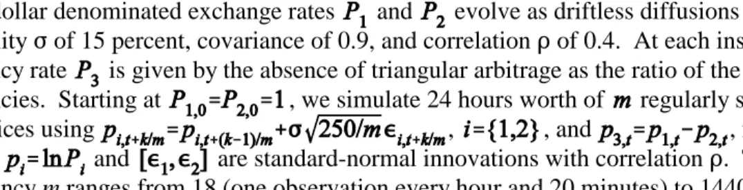
Bid-ask bounce is a well-known reality of financial market data. To examine its effect on the covariance and correlation estimates, we augment the Monte Carlo experiment with a simple model of bid-ask bounce and price discreteness taken from Hasbrouck (1999b). Specifically, we take the dollar rates from the original experiment as the true prices and compute the bid and ask

quotes and , where

and are functions that round down or up to the nearest tick, respectively. For the cross rate, we compute the bid and ask quotes by imposing no-arbitrage given the bid and ask quotes of the dollar rates. We then take the observed prices as , where

. To capture the fact that the two base currencies are denominated in dollars, which means that the sale or purchase of the dollar might involve a simultaneous purchase or sale of the two currencies, we allow the buy-sell indicators and to be correlated with

. The indicator is independent.

Table 2 presents the results for a bid-ask spread of 0.0005 and a tick size of 0.0001, which are realistic values for currencies (see Hasbrouck, 1999b). In Panel A the correlation 0 is

(14)

set to zero and in Panels B the correlation is 0.5. The effect of bid-ask bounce on the range-based estimates is relatively minor. In contrast, the effect on the realized volatilities, covariance, and correlation is striking. Consistent with the intuition outlined above, the realized volatilities are upward biased when the data is sampled more frequently than once every three hours. By the time the data is sampled every minute, the bias inflates the true volatility by almost 100 percent (an average estimate of 29.7 percent as opposed to a true volatility of 15 percent). The results for the realized covariance depend on whether we construct the estimator using the no-arbitrage condition or return cross-products and on the correlation of the bid-ask indicators. If we use the no-arbitrage condition, the realized covariance inherits the biases of the realized volatilities, to the point where for five-minute sampling the average estimate is negative. In contrast, if we use return cross-products and if the bid-ask indicators are independent (in Panel A), the realized covariance is unbiased. The reason is that if the bid-ask indicators are independent, then the expectation of the product of observed returns is equal to the expectation of the product of true returns. The bid-ask bounce therefore only increases the variability of the estimator. However, if the bid-ask indicators are correlated (in Panel B), this argument no longer holds and the realized covariance is severely positively biased because each cross-product of returns contains an upward bias due to the common component of the bid-ask indicators. Finally, the realized correlation, computed from the biased realized volatilities and biased covariance, is unreliable, ranging from -0.89 to 0.66.

Finally, asynchronous trading is another market microstructure effect that is likely to affect differently the range-based and realized covariance and correlation estimates. With infrequent trading, a security has a latent true price that is only revealed when a trade occurs. Between trades, the observed price is stale at the last traded price and therefore does not reflect

(15)

the true price. In a univariate setting, infrequent trading induces positive serial-correlation in the intraday returns, which, in turn, causes a downward bias in the realized volatility. In a bivariate setting, asynchronous infrequent trading, when the trades for the two assets do not take place at the same time, also creates a misalignment of the return-cross products that may lead to a downward bias of the realized covariance.

To capture the effect of asynchronous infrequent trading in our Monte Carlo experiment, we use the discretization (13) with (one observation per second) to simulate the latent “true” price processes. We then assign for each process trade times randomly throughout the day and construct stale price processes for which the price is equal to the price at the previous trade time until it is reset to the latent true price at the next trade time. Hence the true prices look like continuous diffusions while the stale prices look like discrete steps that occur at different times for the different currencies. Finally, we sample these stale price processes at a regular frequency ranging again from four to 1440 and proceed just as in Table 1 (i.e., there is no bid-ask bounce in this experiment).

We present the results for (an average of one trade every minute) in Table 3. The range-based estimates are slightly downward biased because the infrequent trading magnifies the discretization bias. The realized volatilities are slightly downward biased due to the positive serial correlation induced by infrequent trading. Finally, when we compute the realized

covariance and correlation using the no-arbitrage condition, the estimates inherit only the slight bias from infrequent trading, but when we instead use return cross-products, the estimates are severely downward biased. In particular, the average realized covariance and correlation

computed with return cross-products are close to zero in both panels. This extreme bias is due to the asynchronous price revelation.

(16)

5. Conclusion

We have extended the important idea of range-based volatility estimation to the

multivariate case. In particular, we proposed a range-based covariance estimator motivated by financial economic considerations (the absence of arbitrage), in addition to statistical

considerations. We showed that, unlike other univariate and multivariate volatility estimators, the range-based estimator is highly efficient yet robust to market microstructure noise arising from bid-ask bounce and asynchronous trading. Many extensions and applications of the ideas developed here are possible, and Brunetti and Lildolt (2002) take up several.

An intriguing application, which to the best of our knowledge has not yet been explored, involves constructing range-based volatility and covariance bets via a portfolio of lookback options. The payoff of a lookback straddle (a lookback call plus a lookback put) is equal to the range of the underlying asset over the life of the option. Therefore, lookback straddles are ideal for placing bets on the range-based volatility of an asset: their payoffs are high (low) when volatility as measured by the range is high (low). Our no-arbitrage approach to covariance estimation suggests an analogous way of placing bets on the covariance between two assets. Consider a portfolio of a long A/$ lookback straddle, a long B/$ lookback straddle, and a short A/B lookback straddle. Since each of the straddles is a variance bet, the payoffs of this portfolio are high (low) when covariance between the two dollar rates is high (low) over the life of the option.

(17)

References

Alizadeh, Sassan, Michael W. Brandt, and Francis X. Diebold, 2002, Range-based estimation of stochastic volatility models, Journal of Finance 57, 1047-1092.

Andersen, Torben G., and Tim Bollerslev, 1998, Answering the skeptics: Yes, standard volatility models do provide accurate forecasts, International Economic Review 39, 885-905. Andersen, Torben G., Tim Bollerslev, and Francis X. Diebold, 2003, Parametric and

nonparametric volatility measurement, in L.P. Hansen and Y. Ait-Sahalia (eds.), Handbook of Financial Econometrics. Amsterdam: North-Holland, forthcoming.

Andersen, Torben G., Tim Bollerslev, Francis X. Diebold, and Paul Labys, 2003, Modeling and forecasting realized volatility, Econometrica 71, 579-626.

Ball, Clifford A., and Walter N. Torous, 1984, The maximum likelihood estimation of security price volatility: Theory, evidence, and application to option pricing, Journal of Business

57, 97-112.

Beckers, Stan, 1983, Variance of security price returns based on high, low, and closing prices,

Journal of Business 56, 97-112.

Brunetti, Celso, and Peter Lildolt, 2002, Return-based and range-based (co)variance estimation, with an application to foreign exchange markets, manuscript.

Garman, Mark B., and Michael J. Klass, 1980, On the estimation of price volatility from historical data, Journal of Business 53, 67-78.

Gill, Philip E., Walter Murray, and Margaret H. Wright, 1981, Practical Optimization. New York: Academic Press.

Hull, John, and Alan White, 1987, The Pricing of options on assets with stochastic volatilities,

(18)

Kunitomo, Naoto, 1992, Improving the Parkinson methods of estimating security price volatilities,

Journal of Business 65, 295-302.

Ledoit, Olivier, and Michael W. Wolf, 2001, A well-conditioned estimator for large-dimensional covariance matrices, Working Paper, Anderson School of Business, UCLA.

Parkinson, Michael, 1980, The extreme value method for estimating the variance of the rate of return, Journal of Business 53, 61-65.

Rogers, L. Christopher G., and Stephen E. Satchell, 1991, Estimating variance from high, low, and closing prices, Annals of Applied Probability 1, 504-512.

Schnabel, Robert B., and Elizabeth Eskow, 1999, A revised modified Cholesky factorization algorithm, SIAM Journal of Optimization 9, 1135-1148.

Yang, Dennis, and Qiang Zhang, 2000, Drift-independent volatility estimation based on high, low, open, and close prices, Journal of Business 73, 477-491.

(19)

Table 1: Range-Based and Realized Estimates in Merton’s Utopia

Two dollar denominated exchange rates and evolve as driftless diffusions with annualized volatility F of 15 percent, covariance of 0.9, and correlation D of 0.4. At each instant the cross-currency rate is given by the absence of triangular arbitrage as the ratio of the two base currencies. Starting at , we simulate 24 hours worth of regularly spaced intraday

log prices using , , and , for k=1,...m,

where and are standard-normal innovations with correlation D. The sampling frequency m ranges from 18 (one observation every hour and 20 minutes) to 1440 (on

observation every minute). We use this observed data to compute the daily range and intraday returns and then construct three estimates of the volatilities, covariance, and correlation. We construct range-based covariance estimates using Parkinson’s variance estimator and

. We construct realized covariance estimates using either the realized variance estimator and the same expression for the covariance or using the cross-products of intraday returns. We repeat this procedure 10,000 times and report the means, standard deviations, and root mean squared errors.

Sampling Frequency

Standard Deviation Covariance Correlation Mean StdDev RMSE Mean StdDev RMSE Mean StdDev RMSE

Range-Based Estimates 1-min 14.099 4.279 4.373 0.862 1.084 1.085 0.371 0.341 0.342 5-min 13.746 4.277 4.457 0.823 1.061 1.064 0.369 0.351 0.352 10-min 13.477 4.274 4.537 0.794 1.043 1.048 0.368 0.359 0.360 20-min 13.090 4.266 4.674 0.753 1.016 1.026 0.366 0.370 0.372 40-min 12.525 4.255 4.923 0.695 0.977 0.998 0.363 0.389 0.391 1hr 20-min 11.701 4.236 5.369 0.615 0.918 0.961 0.358 0.420 0.422

Realized Estimates with No-Arbitrage Condition

1-min 14.997 0.280 0.280 0.900 0.064 0.064 0.400 0.022 0.022 5-min 14.985 0.623 0.624 0.900 0.143 0.143 0.400 0.050 0.050 10-min 14.971 0.883 0.883 0.901 0.202 0.202 0.399 0.070 0.070 20-min 14.943 1.249 1.250 0.900 0.285 0.285 0.398 0.099 0.099 40-min 14.888 1.758 1.762 0.898 0.404 0.404 0.395 0.142 0.142 1hr 20-min 14.788 2.475 2.484 0.896 0.570 0.570 0.389 0.203 0.203

Realized Estimates with Cross-Products

(20)

Table 2:Range-Based and Realized Estimates with Bid-Ask Bounce We simulate two currency prices as described in Table 1 and then compute the bid and ask

quotes and , where

and are functions that round down or up to the nearest tick, respectively. The spread is set to 0.0005 and the tick size is 0.0001. For the cross-currency, we compute the bid and ask quotes by imposing no-arbitrage given the bid and ask quotes of the base currencies. We then take the observed prices as , where . The buy-sell indicators and are correlated with but the indicator is

independent. In panel A and in panel B . We use this observed data to compute the daily range and intraday returns and then construct three estimates of the volatilities, covariance, and correlation. We construct range-based covariance estimates using Parkinson’s variance

estimator and . We construct realized

covariance estimates using either the realized variance estimator and the same expression for the covariance or using the cross-products of intraday returns. We repeat this procedure 10,000 times and report the means, standard deviations, and root mean squared errors.

Panel A: Independent Bid-Ask Bounce with

Sampling Frequency

1-min 29.645 0.490 14.653 -5.578 0.462 6.495 -0.636 0.060 1.037 5-min 18.849 0.760 3.924 -0.395 0.341 1.339 -0.114 0.100 0.524 10-min 17.010 0.990 2.241 0.253 0.351 0.736 0.082 0.118 0.339 20-min 15.994 1.327 1.658 0.578 0.396 0.511 0.217 0.141 0.231 40-min 15.422 1.820 1.868 0.736 0.486 0.513 0.296 0.177 0.206 1hr 20-min 15.058 2.515 2.516 0.815 0.629 0.635 0.335 0.232 0.241

(21)

Panel B: Correlated Bid-Ask Bounce with

Sampling Frequency

1-min 29.645 0.490 14.653 -7.812 0.548 8.729 -0.890 0.073 1.292 5-min 18.849 0.760 3.924 -0.842 0.375 1.782 -0.241 0.114 0.651 10-min 17.010 0.990 2.241 0.029 0.375 0.949 0.004 0.130 0.417 20-min 15.994 1.327 1.658 0.465 0.414 0.601 0.172 0.151 0.273 40-min 15.422 1.820 1.868 0.679 0.500 0.547 0.270 0.185 0.226 1hr 20-min 15.058 2.515 2.516 0.786 0.640 0.650 0.321 0.238 0.251

(22)

Table 3: Range-Based and Realized Estimates with Asynchronous Trading We simulate 24 hours worth of regularly spaced intraday log prices (one price every second) for three currencies as described in Table 1. We then assign to each log price process

n=1440 trade times (an average of one trade every minute) randomly throughout the day and construct stale price processes for which the price is equal to the price at the previous trade time until it is reset to the latent true price at the next trade time. We then sample these stale price processes at a regular frequency m ranging from 18 (one observation every hour and 20 minutes) to 1440 (one observation every minute). We use this observed data to compute the daily range and intraday returns and then construct three estimates of the volatilities, covariance, and

correlation. We construct range-based covariance estimates using Parkinson’s variance estimator

and . We construct realized covariance

estimates using either the realized variance estimator and the same expression for the covariance or using the cross-products of intraday returns. We repeat this procedure 10,000 times and report the means, standard deviations, and root mean squared errors.

Sampling Frequency