PARALLEL DISCRETE EVENT SIMULATION OF QUEUING NETWORKS USING GPU-BASED HARDWARE ACCELERATION
By
HYUNGWOOK PARK
A DISSERTATION PRESENTED TO THE GRADUATE SCHOOL OF THE UNIVERSITY OF FLORIDA IN PARTIAL FULFILLMENT
OF THE REQUIREMENTS FOR THE DEGREE OF DOCTOR OF PHILOSOPHY
UNIVERSITY OF FLORIDA 2009
c
ACKNOWLEDGMENTS
I would like to express my sincere gratitude to my advisor, Dr. Paul A. Fishwick for his excellent inspiration and guidance throughout my Ph.D. studies at the University of Florida. I would also like to thank my Ph.D. committee members, Dr. Jih-Kwon Peir, Dr. Shigang Chen, Dr. Benjamin C. Lok, and Dr. Howard W. Beck for their precious time and advice for my research. Also, I am grateful to the Korean Army. They gave me a chance to study in the United States of America with financial support. I would like to thank my parents, Hyunkoo Park and Oksoon Jung who encouraged me throughout my studies. I would especially like to thank my wife, Jisuk Han, and my sons, Kyungeon and Sangeon Park. They have been very supportive and patient throughout my studies. I would never have finished my study without them.
TABLE OF CONTENTS page ACKNOWLEDGMENTS . . . 4 LIST OF TABLES. . . 8 LIST OF FIGURES . . . 9 ABSTRACT . . . 11 CHAPTER 1 INTRODUCTION . . . 13
1.1 Motivations and Challenges . . . 13
1.2 Contributions to Knowledge . . . 16
1.2.1 A GPU-Based Toolkit for Discrete Event Simulation Based on Parallel Event Scheduling . . . 16
1.2.2 Mutual Exclusion Mechanism for GPU . . . 16
1.2.3 Event Clustering Algorithm on SIMD Hardware . . . 17
1.2.4 Error Analysis and Correction . . . 18
1.3 Organization of the Dissertation. . . 18
2 BACKGROUND . . . 20
2.1 Queuing Model . . . 20
2.2 Discrete Event Simulation . . . 23
2.2.1 Event Scheduling Method . . . 23
2.2.2 Parallel Discrete Event Simulation . . . 25
2.2.2.1 Conservative synchronization. . . 26
2.2.2.2 Optimistic synchronization . . . 28
2.2.2.3 A comparison of two methods . . . 30
2.3 GPU and CUDA . . . 30
2.3.1 GPU as a Coprocessor. . . 30
2.3.2 Stream Processing . . . 32
2.3.3 GeForce 8800 GTX. . . 33
2.3.4 CUDA . . . 35
3 RELATED WORK . . . 38
3.1 Discrete Event Simulation on SIMD Hardware . . . 38
3.2 Tradeoff between Accuracy and Performance . . . 40
3.3 Concurrent Priority Queue . . . 41
4 A GPU-BASED APPLICATION FRAMEWORK SUPPORTING FAST DISCRETE
EVENT SIMULATION . . . 43
4.1 Parallel Event Scheduling . . . 43
4.2 Issues in a Queuing Model Simulation . . . 45
4.2.1 Mutual Exclusion . . . 45
4.2.2 Selective Update . . . 49
4.2.3 Synchronization . . . 49
4.3 Data Structures and Functions . . . 50
4.3.1 Event Scheduling Method . . . 50
4.3.2 Functions for a Queuing Model . . . 54
4.3.3 Random Number Generation . . . 58
4.4 Steps for Building a Queuing Model . . . 58
4.5 Experimental Results . . . 62
4.5.1 Simulation Environment . . . 62
4.5.2 Simulation Model . . . 62
4.5.3 Parallel Simulation with a Sequential Event Scheduling Method . . 63
4.5.4 Parallel Simulation with a Parallel Event Scheduling Method . . . . 64
4.5.5 Cluster Experiment . . . 65
5 AN ANALYSIS OF QUEUE NETWORK SIMULATION USING GPU-BASED HARDWARE ACCELERATION . . . 67
5.1 Parallel Discrete Event Simulation of Queuing Networks on the GPU . . . 67
5.1.1 A Time-Synchronous/Event Algorithm . . . 67
5.1.2 Timestamp Ordering . . . 69
5.2 Implementation and Analysis of Queuing Network Simulation . . . 70
5.2.1 Closed and Open Queuing Networks . . . 70
5.2.2 Computer Network Model . . . 72
5.2.3 CUDA Implementation . . . 74
5.3 Experimental Results . . . 76
5.3.1 Simulation Model: Closed and Open Queuing Networks . . . 76
5.3.1.1 Accuracy: closed vs. open queuing network . . . 77
5.3.1.2 Accuracy: effects of parameter settings on accuracy . . . 79
5.3.1.3 Performance . . . 79
5.3.2 Computer Network Model: a Mobile Ad Hoc Network . . . 83
5.3.2.1 Simulation model . . . 83
5.3.2.2 Accuracy and performance . . . 86
5.4 Error Analysis . . . 88
6 CONCLUSION . . . 95
6.1 Summary . . . 95
6.2 Future Research . . . 96
LIST OF TABLES
Table page
2-1 Notations for queuing model statistics . . . 22
2-2 Equations for key queuing model statistics . . . 23
3-1 Classification of parallel simulation examples . . . 42
4-1 The future event list and its attributes. . . 51
4-2 The service facility and its attributes . . . 55
5-1 Simulation scenarios of MANET . . . 86
5-2 Utilization and sojourn time (Soj.time) for different values of time intervals (t) and mean service times (s) . . . 91
LIST OF FIGURES
Figure page
2-1 Components of a single server queuing model . . . 21
2-2 Cycle used for event scheduling . . . 24
2-3 Stream and kernel . . . 33
2-4 Traditional vs. GeForce 8 series GPU pipeline. . . 34
2-5 GeForce 8800 GTX architecture . . . 35
2-6 Execution between the host and the device . . . 37
3-1 Diagram of parallel simulation problem space . . . 42
4-1 The algorithm for parallel event scheduling . . . 44
4-2 The result of a concurrent request from two threads without a mutual exclusion algorithm . . . 46
4-3 A mutual exclusion algorithm with clustering events. . . 48
4-4 Pseudocode forNextEventTime . . . 52
4-5 Pseudocode forNextEvent . . . 53
4-6 Pseudocode forSchedule . . . 54
4-7 Pseudocode forRequest . . . 55
4-8 Pseudocode forRelease . . . 56
4-9 Pseudocode forScheduleServer . . . 57
4-10 First step in parallel reduction . . . 59
4-11 Steps in parallel reduction . . . 59
4-12 Step 3: Event extraction and departure event . . . 60
4-13 Step 4: Update of service facility . . . 61
4-14 Step 5: New event scheduling . . . 61
4-15 3×3 toroidal queuing network . . . 63
4-16 Performance improvement by using a GPU as coprocessor . . . 64
5-1 Pseudocode for a hybrid time-synchronous/event algorithm with parallel event
scheduling . . . 68
5-2 Queuing delay in the computer network model . . . 73
5-3 3 linear queuing networks with 3 servers . . . 76
5-4 Summary statistics of closed and open queuing network simulations . . . 78
5-5 Summary statistics with varying parameter settings . . . 80
5-6 Performance improvement with varying time intervals (t) . . . 82
5-7 Comparison between wireless and mobile ad hoc networks . . . 84
5-8 Average end-to-end delay with varying time intervals (t) . . . 87
5-9 Average hop counts and packet delivery ratio with varying time intervals (t) . 89 5-10 Performance improvement in MANET simulation with varying time intervals (t) 90 5-11 3-dimensional representation of utilization for varying time intervals and mean service times . . . 91
5-12 Comparison between experimental and estimation results . . . 93
Abstract of dissertation Presented to the Graduate School of the University of Florida in Partial Fulfillment of the Requirements for the Degree of Doctor of Philosophy
PARALLEL DISCRETE EVENT SIMULATION OF QUEUING NETWORKS USING GPU-BASED HARDWARE ACCELERATION
By
Hyungwook Park December 2009 Chair: Paul A. Fishwick
Major: Computer Engineering
Queuing networks are used widely in computer simulation studies. Examples of queuing networks can be found in areas such as the supply chains, manufacturing work flow, and internet routing. If the networks are fairly small in size and complexity, it is possible to create discrete event simulations of the networks without incurring significant delays in analyzing the system. However, as the networks grow in size, such analysis can be time consuming and thus require more expensive parallel processing computers or clusters.
The trend in computing architectures has been toward multicore central processing units (CPUs) and graphics processing units (GPUs). A GPU is the fairly inexpensive hardware, and found in most recent computing platforms, but practical example of single instruction, multiple data (SIMD) architectures. The majority of studies using the GPU within the graphics and simulation communities have focused on the use of the GPU for models that are traditionally simulated using regular time increments, whether these increments are accomplished through the addition of a time delta (i.e., numerical integration) or event scheduling using the delta (i.e., discrete event approximations of continuous-time systems). These types of models have the property of being decomposable over a variable or parameter space. In prior studies, discrete event simulation, such as a queuing network simulation, has been characterized as being an inefficient application for the GPU primarily due to the inherent synchronicity of
the GPU organization and an apparent mismatch between the classic event scheduling cycle and the GPUs basic functionality. However, we have found that irregular time advances of the sort common in discrete event models can be successfully mapped to a GPU, thus making it possible to execute discrete event systems on an inexpensive personal computer platform.
This dissertation introduces a set of tools that allows the analyst to simulate
queuing networks in parallel using a GPU. We then present an analysis of a GPU-based algorithm, describing benefits and issues with the GPU approach. The algorithm
clusters events, achieving speedup at the expense of an approximation error which grows as the cluster size increases. We were able to achieve 10-x speedup using our approach with a small error in the output statistics of the general network topology. This error can be mitigated, based on error analysis trends, obtaining reasonably accurate output statistics.
CHAPTER 1 INTRODUCTION
1.1 Motivations and Challenges
Queuing models [1–4] are constructed to analyze humanly engineered systems where jobs, parts, or people flow through a network of nodes (i.e. resources). The study of queuing models, their simulation, and their analysis is one of the primary research topics studied within the discrete event simulation community [5]. There are two approaches to estimating the performance and analysis of queuing systems: analytical modeling and simulation [3,5,6]. An analytical model is the abstraction of a system based on probability theory, representing the description of a formal system consisting of equations used to estimate the performance of the system. However, it is difficult to represent all situations in the real world using an analytical model because that requires a restricted set of assumptions, such as an infinite number of queue capacity and no bounds on the inter-arrival and service time, which do not often occur in the real world. A simulation is often used to analyze the queuing system when a theory for the system equations is unknown or the algorithm for the equations is too complicated to be solved in closed-form. Computer simulation involves the formulation of a mathematical model, often including a diagram. This model is then translated into computer code, which is then executed and compared against a physical, or real-world, system’s behavior under a variety of conditions.
Queuing model simulations can be expensive in terms of time and resources in cases where the models are composed of multiple resource nodes and tokens that flow through the system. Therefore, there is a need to find ways to speed up queuing model simulations so that analyses can be obtained more quickly. Past approaches to speeding up queuing model simulations have used asynchronous message-passing with special emphasis on two approaches: the conservative and the optimistic approaches [7]. Both approaches have been used to synchronize the asynchronous
logical processors (LPs), preserving causal relationships across LPs so that the results obtained are exactly the same as those produced by sequential simulation. Most studies of parallel simulation have been performed on multiple instruction, multiple data (MIMD) machines, or related networks to execute the part of a simulation model or LP. The parallel simulation approaches with partitioning the simulation model into several LPs could easily be employed with a queuing model simulation, since the start of each execution need not be explicitly synchronized with other LPs.
A graphics processing unit (GPU) is a processor that renders 3D graphics in real time, and which contains several sub-processing units. Recently, the GPU has become an increasingly attractive architecture for solving compute-intensive problems for general purpose computation, which is called general-purpose computation on GPUs (GPGPU) [8–11]. Availability as a commodity and increased computational power make the GPU a substitute for expensive clusters of workstations in a parallel simulation, at a relatively low cost. For much of the history of GPU development, there has been a need to map the model into the graphics application programming interface (API), which limited the availability of the GPU to those experts who had GPU- and graphics-specific knowledge. This drawback has been resolved with the advent of the GeForce 8 series GPUs [12] and compute unified device architecture (CUDA) [13,14]. The control of the unified stream processors on the GeForce 8 series GPUs is transparent to the programmer, and CUDA provides an efficient environment to develop parallel codes in a high-level language C without the need for graphics-specific knowledge.
In contrast to the previously ubiquitous MIMD approach to parallel computation within the context of simulation research, the GPU is single instruction, multiple data (SIMD)-based hardware that is oriented toward stream processing. SIMD hardware is a relatively simple, inexpensive, and highly parallel architecture; however, there are limits to developing an asynchronous model due to its synchronous operation. Stream processing [15,16] is the basic programming model of SIMD architecture. The
stream processing approach exploits data and task parallelism by mapping data flow to processors, and provides efficient communication by accessing memory in a predictable pattern using a producer-consumer locality as well. For these reasons, most simulation models on the GPU are time-synchronous and compute-intensive models with stream memory access.
However, queuing models are a typical asynchronous model, and their temporal events are relatively fine-grained. Queuing models are usually simulated based on event scheduling with manipulation of the future event list (FEL). Event scheduling tends to be a sequential operation, which often overwhelms the execution times of events in queuing model simulations. Another problem lies in the dynamic data structure for the event scheduling method in discrete event simulations. Dynamic data structures cannot be directly used on the GPU because dynamic memory allocation is not supported during kernel execution. Moreover, the randomized memory access for individual data cannot take advantage of massive parallelism on the GPU.
Nonetheless, the GPU can become useful hardware for facilitating fine-grained discrete event simulations, especially for large-scale models, with the concurrent utilization of a number of threads and fast data transfer between processors. The execution time of each event can be very small, but a higher data parallelism with clustering of the events can be achieved for a large-scale model.
The objective of this dissertation is to simulate asynchronous queuing networks using GPU-based hardware acceleration. Two main issues related to this study are: (1) how can we simulate asynchronous models on SIMD hardware? And (2) how can we achieve a higher degree of parallelism? Investigations of these two main issues reveal that further attention must be paid to the following related issues: (a) parallel event scheduling, (b) data consistency without explicit support for mutual exclusion, (c) event clustering, and (d) error estimation and correction. This dissertation presents an approach to resolve these challenges.
1.2 Contributions to Knowledge
1.2.1 A GPU-Based Toolkit for Discrete Event Simulation Based on Parallel Event Scheduling
We have developed GPU-based simulation libraries for CUDA so that the GPU can easily be used for discrete event simulation, especially for a queuing network simulation. A GPU is designed to process array-based data structures for the purpose of processing pixel images in real time. The framework includes the functions for event scheduling and queuing models that have been developed using arrays on the GPU.
In discrete event simulation, the event scheduling method occupies a large portion of the overall simulation time. The FEL implementation, therefore, needs to be parallelized in order to take full advantage of the GPU architecture. A concurrent priority queue approach [17,18] allows each processor to access the global FEL in parallel on shared memory multiprocessors. The concurrent priority queue approach, however, cannot be directly applied to SIMD-based hardware since the concurrent insertion and deletion of the priority queue usually involves mutual exclusion, which is not natively supported by GeForce 8800 GTX GPU [13].
Parallel event scheduling allows us to achieve significant speedup in queuing model simulations on the GPU. A GPU has many threads executed in parallel, and each thread can concurrently access the FEL. If the FEL is decomposed into many sub-FELs, and each sub-FEL is exclusively accessed by one thread, the access to one element in the FEL is guaranteed to be isolated from other threads. Exclusive access to each element allows event insertion and deletion to be concurrently executed.
1.2.2 Mutual Exclusion Mechanism for GPU
We have reorganized the processing steps in a queuing model simulation by employing alternate updates between the FEL and service facilities so that they can be updated in SIMD fashion. The new procedure enables us to prevent multiple threads
from simultaneously accessing the same element, without having explicit support for mutual exclusion on the GPU.
An alternate update is a lock-free method for mutual exclusion on the GPU, in order to update two interactive arrays at the same time. Only one array can be exclusively accessed by a thread index if the indexes of two arrays are not inter-related. If one array needs to update the other array, the element in the other array is arbitrarily accessed by the thread. Data consistency cannot be maintained if two or more threads concurrently access the same element in the other array. The other array must be updated after the thread index is switched to exclusively access itself. The updated array, however, has to search all of the elements in the request array to find the request elements. If the updated array knows which elements in the request array are likely to request the update in advance, the number of searches will be limited. Each node in queuing networks usually knows its incoming edges, which makes it possible to reduce the number of searches during an alternate update, mitigating the overall execution time.
1.2.3 Event Clustering Algorithm on SIMD Hardware
SIMD-based simulation is useful when a lot of computation is required by a single instruction with different data. However, its potential problems include the bottleneck in the control processor and load imbalance among processors. The bottleneck problem should not be significant when applying the CPU/GPU approach, since the CPU is designed to process heavyweight threads, whereas the GPU is designed to process lightweight threads and to execute arithmetic equations quickly [16].
The load imbalance problem can be resolved by employing a time-synchronous/event algorithm in order to achieve a higher degree of parallelism. A single timestamp cannot execute many events in parallel, since events in queuing models are irregularly spaced. Thus, event times need to be modified so that they can be clustered and synchronized. A time-synchronous/event algorithm is the SIMD-based hybrid approach to two common types of discrete simulation: discrete event and time-stepped. The algorithm adopts the
advantages of both methods to utilize the GPU. The simulation clock advances when the event occurs, but the events in the middle of the time interval are executed concurrently. A time-synchronous/event algorithm naturally leads to approximation errors in the summary statistics yielded from the simulation, because the events are not executed at their precise timestamp.
We investigated three different types of queuing models to observe the effects of our simulation method, including an implementation of a real-world application (mobile ad hoc network model). The experimental results of our investigation show that our algorithm has different impacts on the statistical results and performance of three types of queuing models.
1.2.4 Error Analysis and Correction
The error in our simulation is a numerical error since we preserves timestamp ordering and causal relationships of events, and the result is approximate in terms of gathered summary statistics. The error may be acceptable for those modeled
applications where the analyst is more concerned with speed, and can accept relatively small inaccuracies in summary statistics. In some cases, the error can be approximated and potentially corrected to yield more accurate statistics. We present a method for estimating the potential error incurred through event clustering by combining queuing theory and simulation results. This method can be used to obtain a closer approximation to the summary statistics through partially correcting the error.
1.3 Organization of the Dissertation
This dissertation is organized into 6 chapters. Chapter 2 reviews background information, including the queuing model, sequential and parallel discrete event simulation, GPU, and CUDA. Chapter 3 describes related work. We discuss other studies for discrete event simulation on SIMD hardware, and a tradeoff between
accuracy and performance. Chapter 4 describes a GPU-based library and applications framework for discrete event simulation. We introduce the routines that support parallel
event scheduling with mutual exclusion and queuing model simulations. Chapter 5 discusses a theoretical methodology and its performance analysis, including the tradeoffs between numerical errors and performance gain, as well as the approaches for error estimation and correction. Chapter 6 provides a summary of our findings and introduces areas for future research.
CHAPTER 2 BACKGROUND
2.1 Queuing Model
Queues are commonly found in most human-engineered systems where there exist one or more shared resources. Any system where the customer requests a service for a finite-capacity resource may be considered to be a queuing system [1]. The grocery store, theme parks, and fast-food restaurants are well-known examples of queuing systems. A queuing system can also be referred to as a system of flow. A new customer enters the queuing system and joins the queue (i.e., line) of customers unless there is no queue and another customer who completes his service may exit the system at the same time. During the execution, a waiting line is formed in a system because the arrival time of each customer is not predictable, and the service time often exceeds customer inter-arrival times. A significant number of arrivals make each customer to wait in line longer than usual. Queuing models are constructed by a scientist or engineer to analyze the performance of a dynamic system where waiting can occur. In general, the goals of a queuing model are to minimize the average number of waiting customers in a queue and to predict the estimated number of facilities in a queuing system. The performance results of queuing model simulation are produced at the end of a simulation in the form of aggregate statistics.
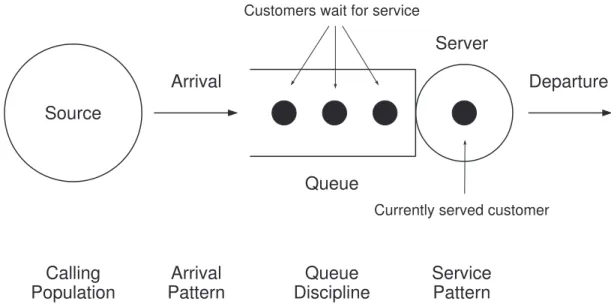
A queuing model is described by its attributes [2,6]: customer population, arrival and service pattern, queue discipline, queue capacity, and the number of servers. A new customer from the calling population enters into the queuing model and waits for service in the queue. If the queue is empty and the server is idle, a new customer is immediately sent to the server for service, otherwise the customer remains in the queue joining the waiting line until the queue is empty and the server becomes idle. When a customer enters into the server, the status of the server becomes busy, not allowing any more
Source
Arrival Departure
Customers wait for service
Queue
Server
Currently served customer
Calling Population Arrival Pattern Queue Discipline Service Pattern
Figure 2-1. Components of a single server queuing model
arrivals to gain access to the server. After being served, a customer exits the system. Figure2-1illustrates a single server queue with its attributes.
The calling population, which can be either finite or infinite, is defined as the pool of customers who possibly can request the service in the near future. If the size of the calling population is infinite, the arrival rate is not affected by others. But the arrival rate varies according to the number of customers who have arrived if the size of the calling population is finite and small. Arrival and service patterns are the two most important factors determining behaviors of queuing models. A queuing model may be deterministic or stochastic. For the stochastic case, new arrivals occur in a random pattern and their service time is obtained by probability distribution. The arrival and service rates, based on observation, are provided as the values of parameters for stochastic queuing models. The arrival rate is defined as the mean number of customers per unit time, and the service rate is defined by the capacity of the server in the queuing model. If the service rate is less than the arrival rate, the size of the queue will grow infinitely. The arrival rate must be less than the service rate in order to maintain a stable queuing system [1,6].
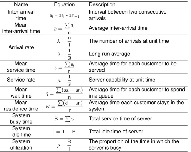
Table 2-1. Notations for queuing model statistics Notation Description
ari Arrival time for customeri ai Inter-arrival time for customeri
a Average inter-arrival time 𝜆 Arrival rate
T Total simulation time
n Number of arrived customers si Service time ofith customer
𝜇 Service rate
ssi Service start time ofith customer di Departure time ofith customer
q Mean wait time
w Mean residence time 𝜌 Utilization
B System busy time I System idle time
The randomness of arrival and service patterns cause the length of waiting lines in the queue to vary.
When a server becomes idle, the next customer is selected among candidates from the queue. The selection of strategy from the queue is called queue discipline. Queue discipline [6,19] is a scheduling algorithm to select the next customer from the queue. The common algorithms of queue discipline are first-in first-out (FIFO), last-in first-out (LIFO), service in random order (SIRO), and priority queue. The earlier arrived customer is usually selected from a queue in the real world, thus the most common queue discipline is FIFO. In a priority queue discipline, each arrival has its priority. The arrival that has the highest priority is chosen from queue among waiting customers.
The purpose of building a queuing model and running a simulation is to obtain meaningful statistics such as the server performance. The notations used for statistics are listed in Table2-1, and the equations for key statistics are summarized in Table2-2.
Table 2-2. Equations for key queuing model statistics
Name Equation Description
Inter-arrival a
i =ari -ari−1 Interval between two consecutive
time arrivals
Mean
a = ∑
ai
n Average inter-arrival time inter-arrival time
Arrival rate
𝜆= Tn The number of arrivals at unit time 𝜆 = 1a Long run average
Mean
s = ∑
si n
Average time for each customer to be
service time served
Service rate 𝜇= 1
s Server capability at unit time Mean
q = ∑
(ssi−ari) n
Average time for each customer to spend
wait time in a queue
Mean w = ∑ (di−ari) n
Average time each customer stays in the
residence time system
System
B = ∑si Total service time of server
busy time System
I = T−B Total idle time of server idle time
System
𝜌= BT The proportion of the time in which the
utilization server is busy
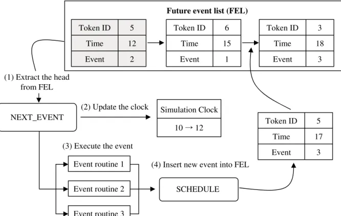
2.2 Discrete Event Simulation
2.2.1 Event Scheduling Method
Discrete event simulation changes the state variables at a discrete time when the event occurs. An event scheduling method [20] is the basic paradigm for discrete event simulation and is used along with a time-advanced algorithm. The simulation clock indicates the current simulated time, the event time of last event occurrence. The unprocessed, or future, events are stored in a data structure called the FEL. Events in the FEL are usually sorted in non-decreasing timestamp order. When the simulation starts, the head of the FEL is extracted from the FEL, updating the simulation clock. The extracted event is then sent to an event routine, where it reproduces a new event after
(2) Update the clock
Event routine 1
Event routine 2
Event routine 3
Future event list (FEL)
NEXT_EVENT Simulation Clock
10 ˧12 SCHEDULE Token ID 5 Time 12 Event 2 Token ID 6 Time 15 Event 1 Token ID 3 Time 18 Event 3
(3) Execute the event
Token ID 5
Time 17
Event 3
(4) Insert new event into FEL (1) Extract the head
from FEL
Figure 2-2. Cycle used for event scheduling
its execution. The new event is inserted to the FEL, sorting the FEL in non-decreasing timestamp order. This step is iterated until the simulation ends.
Figure2-2illustrates the basic cycle for event scheduling [20]. Three future events are stored into the FEL. When NEXT EVENT is called, token ID #5 with timestamp 12 is extracted from the head of the FEL. The simulation clock then advances from 10 to 12. The event is executed at event routine 2, which creates a new future event, event #3. Token ID #5 with event #3 is scheduled and inserted into the FEL. Token ID #5 is placed between token ID #6 and token ID #3 after comparing their timestamps. The event loop iterates to call NEXT EVENT until the simulation ends.
The priority queue is the abstract data structure for an FEL. The priority queue involves two operations for processing and maintaining the FEL: insert and delete-min. The simplest way to implement the priority queue is to use an array or a linked list. These data structures store events in a linear order by event time but are inefficient
for large-scale models, since the newly inserted event compares its event time with all others in the sequence. An array and linked list takes O(N) time for insertion, and O(1) time for deletion on average, whereN is the number of elements in these data structures. When an event is inserted, an array can be accessed faster than a linked list on the disk, since the elements in arrays are stored contiguously. On the other hand, an FEL using an array requires its own dynamic storage management [20].
The heap and splay tree [21] are data structures typically used for an FEL. They are tree-based data structures and can execute operations faster than linear data structure, such an array. Min heap implemented in a height-balanced binary search tree takes O(log N) time for both insertion and deletion. A splay tree is a self-balancing binary tree, but a certain elements can rearrange the tree, placing that element into the root. This makes recently accessed elements able to be quickly referenced again. The splay tree performs both operations in O(log N) amortized time. Heap and splay tree are therefore suitable data structures for a priority queue for a large-scale model.
Calendar queues [22] are operated by a hash function, which performs both operations in O(1), on average. Each bucket is a day that has a specific range and each has a specific data structure for storing events in timestamp order. Enqueue and dequeue functions are operated by hash functions according to event time. The number of buckets and ranges in a day are adjusted to operate the hash function efficiently. Calendar queues are efficient when events are equally distributed to each bucket, which minimizes the adjustment of bucket size.
2.2.2 Parallel Discrete Event Simulation
In traditional parallel discrete event simulation (PDES) [7,23,24], the model is decomposed into several LPs, and each LP is assigned to a processor used for parallel simulation. Each LP runs its own independent part of the simulation with local clock and state variables. When LPs need to communicate with each other, they send timestamped messages to each other over a system bus or via a networking system.
Each local clock advances at different paces because the interval between consecutive events on the LP is irregular. For this reason, the timestamp of incoming events from other LPs can be earlier than the currently executed event. It is called a causality error if the incoming events are supposed to change the state variable to which the current event is referring. The violation of the causality error can produce different results. As a result, a synchronization method needs to process events in a non-decreasing timestamp order and to preserve causal relationships across processors. The performance gains are not proportional to the increased number of processors due to the synchronization overhead. Conservative and optimistic approaches are two main categories in synchronization.
2.2.2.1 Conservative synchronization
In conservative synchronization methods, each processor executes events when it can guarantee that other processors will not send events with a smaller timestamp than that of the current event. Conservative methods can cause a deadlock situation between LPs because every LP can block the event if it is considered to be unsafe to process. Deadlock avoidance, and deadlock detection and recovery are two major challenges of conservative synchronization methods.
Chandy and Misra [25] and Bryant [26] developed a deadlock avoidance algorithm. The necessary and sufficient condition is that the messages are sent to other LPs over the links in non-decreasing timestamp order, which guarantees that the processor will not receive an event with a lower timestamp than the previous one. A null message is sent to avoid the deadlock, indicating that the processor will not send a timestamped message smaller than a null message. The timestamp of a null message is determined by each incoming link, which provides the lower bound of the timestamp when the next event occurs. The lower bound is determined by the knowledge of the simulation such as lookahead, or the minimum timestamp increment for a message passing between LPs. The variations of the null message method tried to reduce the number of null
messages based on demand since the amount of null message traffic can degrade performance [27].
The deadlock detection and recovery proposed by Chandy and Misra [28] tried to eliminate the use of null messages. The deadlock recovery approach allows the processors to become deadlocked. When the deadlock is detected, the recovery function is called. A controller, used to break the deadlock, identifies the event containing the smallest timestamp among the processors, and sends the messages to that LP indicating that the event is safe to process.
Barrier synchronization is one of the conservative synchronization approaches. The lower bound on the timestamp (LBTS1 ) is calculated, based on the time of the next event, and lookahead determines the time when all processors stop the execution to safely process the event. The events are executed only if the timestamps of events are less than LBTS. The distance between LPs is often used to determine LBTS since it implies the minimum time to transmit the event from one LP to another, such as air traffic simulation.
Conservative approaches are easy to implement but performance relies on
lookahead. Lookahead is the minimum time increment when the new event is scheduled, thus lookahead (L) guarantees that no other events containing a smaller timestamp are generated until the current clock plusL. Lookahead is used to predict the next incoming events from other processors when the processor determines if the current event is safe. If the lookahead is too small or zero, the currently executed event can cause all events on the other LPs to wait. In this case, the events are nearly executed in sequential.
1LBTS is defined as ”Lower bound on the timestamp of any message LP can receive in the future” in [7] p77.
2.2.2.2 Optimistic synchronization
In optimistic methods, each processor executes its own events regardless of those received from other processors. However, each processor has to roll back the simulation when it detects a causality error from event execution in order to recover the system. Rollback in a parallel computing environment is a complicated process because some of the messages sent to other LPs also need to be canceled.
Time-warp [29] is the most well-known scheme in optimistic synchronization. Time warp has two major parts: the local and global control mechanisms. The local control mechanism assumes that each local processor executes the events in timestamp order using its own local virtual clock. When an LP sends a message to others, the identical message, except for one field, is created. The original message sent from the LPs has a positive sign, and its corresponding copy, called antimessage, has a negative. Each LP maintains three queues. State queue contains the snapshots of the recent states at an instant in time in the LP. The state is changed whenever the event occurs, and enqueued at the state queue. Received messages from other LPs are stored at an input queue in the timestamp order. The antimessage, produced by its own LP, is stored at the output queue. When the timestamp of the arrival event is earlier than the local virtual time of the LP, the LP encounters the causality error. The state is restored from state queue prior to the timestamp of the current arrival message. Antimessages are dequeued from the output queue and sent to other LPs, if their timestamps are between the arrival event and the local virtual time. When the LP receives an antimessage, they annihilate each other to cancel future events if the input queue contains the corresponding positive message. The LP is rolled back by an antimessage if the corresponding positive
messages are already executed.
Global virtual time (GVT) gives an idea to solve some problems on local control of the Time Warp mechanism, such as the memory management, the global control of rollback and the safe commitment time. The GVT is defined by the minimum of
local virtual time among LPs and the timestamp of messages in transit, and serves as a lower bound for the virtual times of the LPs. GVT allows the efficient memory
management because it does not need to maintain the previous states if those execution times are earlier than the GVT. Duplicate antimessages are often produced while the LP reevaluates the antimessages causing the problem of performance. The Lazy
cancelation waits to send the antimessage until the LP checks to see if the re-execution produces the same messages, whereas Lazy reevaluation uses state vectors, instead of messages, to solve this problem [7].
In the optimistic approach, the past states are saved for recovery, but it has one of the most significant drawbacks regarding memory management. State saving [30] makes copies of the past states during simulation. Copy state saving (CSS) copies the entire states of simulation before each event occurs. CSS is the easiest method for state saving, but two drawbacks are the huge memory consumption to save the entire states and the performance overhead during rollback. Periodic state saving (PSS) sets the checkpoint by interval skipping a few events. The performance is improved with PSS, but all state values still have to be saved at the checkpoint. Incremental state saving (ISS) is the method based on backtracking. Only the values and address of modified variables are stored before the events execute. The old values are written to the variables in reverse order when the states need to be restored. ISS reduces the memory consumption and execution overheads, but the programmer has to add the modules to handle each variable.
Reverse computation (RC) [31] was proposed to solve the limitation of the state saving method for forward computation. RC does not save the values of state variables during simulation. Computation is performed in reverse order to recover the values of state variables until it reaches the checkpoint when the rollback is initiated. RC uses the bit variable to check the changes, thus it can drastically reduce the memory consumption during simulation for especially fine-grained models.
2.2.2.3 A comparison of two methods
Each synchronization approach has a drawback [32]. It takes considerable time to run a simulation with zero lookahead in the conservative method. It is also too difficult to roll back a simulation system to the previous state without error if we run the simulation with a complicated model using the optimistic method. In general, the optimistic method has an advantage over the conservative in that the execution is allowed where a
causality error is possible, but actually does not exist. In addition, the conservative method often needs specific information for the application to determine when it is safe to process the events, but it is not very relevant to an optimistic approach [23]. In some cases, a very small lookahead cannot continue the simulation in parallel, but can in sequential. Finding the lookahead and its size can be critical factors to determine the performance gains in the conservative method [24]. However, optimistic mechanism is much more complex to implement, and frequent rollback causes more computation overhead for a compute-intensive system. If the model is too complex to apply the optimistic method, the conservative method is a better choice. On the other hand, if a very small lookahead is expected, the optimistic method has to be applied.
2.3 GPU and CUDA
2.3.1 GPU as a Coprocessor
A GPU is a dedicated graphics processor that renders 3D graphics in real time, which requires tremendous computational power. The computation speed of the GeForce 8800 GTX is approximately four times faster than that of an Intel Core2 Quad processor with 3.0 GHz, which is approximately twice as expensive as the
GeForce 8800 GTX [13]. The increment of the CPU clock speed has slowed since 2003 due to the physical limitations, so Intel and AMD turned their intention to multi-core architectures [33]. On the other hand, the increment of GPU speed is still growing because more transistors can be used for parallel data processing than data caching and flow control on the GPU. Programmability is another reason that the GPU has
become attractive. The vertex and fragment processors can be customized with the user’s own program.
The GPU has different features compared to the CPU [16]. The CPU is designed to process general purpose programs. For this reason, CPU programming models and their processes are generally serial, and the CPU enables the complex branch controls. The GPU, however, is dedicated to processing the pixel image in real time, thus it has much more parallelism than the CPU does. The CPU returns memory reference quickly to process as many jobs as possible, maximizing its throughput and minimizing the memory latency. As a result, a single thread on a CPU can produce higher performance compared to that on a GPU. On the other hand, the GPU maximizes the parallelism through threads. The performance of a single thread on a GPU is not as good, compared to that on a CPU, but the executions of threads in a massively parallel hide the memory latency to produce high throughput from parallel tasks. In addition, more transistors are dedicated to GPU for data computation rather than data caching and flow control. The GPU can take a great advantage over a CPU when the cache miss occurs [34].
Despite many advantages, the harnessing power of the GPU has been considered to be difficult because GPU-specific knowledge, such as graphics APIs and hardware, needs to deal with the programmable GPU. The traditional GPUs have two types of programmable processors: vertex and fragment [35]. Vertex processors transform the streams of vertices which are defined by positions, colors, textures and lighting. The transformed vertices are converted into fragments by the rasterizer. Fragment processors compute the color of each pixel to render the image. Graphics shader programming languages, such as Cg [36] and HLSL [37], allow the programmer to write the code for the vertex and fragment processors in high-level programming language. Those languages are easy to learn, compared to assembly language, but are still graphic-specific assuming that the user has the basic knowledge of interactive graphic
programming. The program, therefore, needs to be written in a graphics fashion using texture and pixel by mapping the computational variables to graphics primitives using graphics API [38], such as DirectX or OpenGL even for general purpose computations.
Another problem was the constrained memory layout and access. The indirect write or scatter operation was not possible because there is no write instruction in the fragment processor [39]. As a result, the implementation of sparse data structure, such as list and tree, where scattering is required, is problematic removing the flexibility in programming. The CPU can handle the memory easily because it has the unified memory model, but it is not trivial on the GPU because memory cannot be written
anywhere [35]. Finally, the advent of the GeForce 8800 GTX GPU and CUDA eliminates the limitations and provides an easy solution to the programmer.
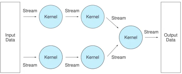
2.3.2 Stream Processing
Stream processing [15,16] is the basis of the GPU programming model today. The application of stream processing is divided into several parts for parallel processing. Each part is referred to as a kernel, which is a programmed function to process the stream and is independent of the incoming stream. The stream is a sequence of elements composed of the same type and it requires the same instruction for
computation. Figure2-3shows the relationship between the stream and the kernel. The stream processing model can process the input stream on each ALU at the same kernel in parallel since each element of input stream is independent of each other. Also, stream processing allows many streams to be processed concurrently at different kernels, which hides the memory latency and communication delay. However, the stream processing model is less flexible and not suitable for the general purpose program with the randomized data access because the stream is directly passed to other kernels connected in sequential after it is processed. Stream processing can consist of several stages, each of which has several kernels. Data parallelism is exploited by processing
Input Data Kernel Kernel Kernel Kernel Kernel Kernel Kernel
Kernel OutputData Stream Stream Stream Stream Stream Stream Stream
Figure 2-3. Stream and kernel
many streams in parallel at each stage and task parallelism is exploited by running several stages concurrently.
Many cores can be utilized concurrently with a stream programming model. For example, GeForce 8800 GTX has 16 multiprocessors, and each can have the maximum 768 threads. Theoretically, approximately ten thousand threads can be executed in parallel yielding high performance parallelism.
2.3.3 GeForce 8800 GTX
The GeForce 8800 GTX [12,13] GPU is the first GPU model unifying vertex, geometry and fragment shaders into 128 individual stream processors. The previous GPUs have the classic pipeline model with a number of stages to render the image from the vertices. Many passes inside the GPU consume the bandwidth. Moreover, some stages are not required to process general purpose computations, which degrade the performance of the processing of the general purpose workloads on the GPU. Figure2-4[40] illustrates the difference of pipeline stages between the traditional and GeForce 8 series GPUs. In GeForce 8800 GTX GPU, the shaders have been unified into the stream processors, which reduce the number of pipeline stages and change the sequential processing into loop-oriented processing. Unified stream processors help to improve load balancing. Any graphical data can be assigned to any available
Application Display Application Display Fragment Rasterization Vertex/Geometry Command Command Rasterization Stream Processors Programmable Processors
Figure 2-4. Traditional vs. GeForce 8 series GPU pipeline
stream processor, and its output stream can be used as an input stream of other stream processors.
Figure2-5[41] shows the GeForce 8800 GTX architecture. The GPU consists of 16 stream multiprocessors (SMs). Each SM has 8 stream processors (SPs), which makes a total of 128. Each SP contains a single arithmetic unit that supports IEEE 754 single-precision floating-point arithmetic and 32-bit integer operations, and can process the instruction in SIMD fashion. Each SM can take up to 8 blocks or 768 threads, which makes for a total of 12,288 threads, and 8192 registers on each SM can be dynamically allocated into the threads running on it.
SP SM Instruction Unit Shared Memory SP SM Instruction Unit Shared Memory SP SM Instruction Unit Shared Memory SP SM Instruction Unit Shared Memory SP SM Instruction Unit Shared Memory SP SM Instruction Unit Shared Memory SP SM Instruction Unit Shared Memory SP SM Instruction Unit Shared Memory SP SM Instruction Unit Shared Memory SP SM Instruction Unit Shared Memory SP SM Instruction Unit Shared Memory SP SM Instruction Unit Shared Memory SP SM Instruction Unit Shared Memory SP SM Instruction Unit Shared Memory SP SM Instruction Unit Shared Memory SP SM Instruction Unit Shared Memory Global Memory Thread Execution Manager
Figure 2-5. GeForce 8800 GTX architecture
2.3.4 CUDA
CUDA [13] is an API of C programming language for utilizing the NVIDIA class of GPUs. CUDA, therefore, does not require a tough learning curve and provides a simplified solution for those who are not familiar with the knowledge of graphics hardware and API. The user can focus on the algorithm itself rather than on its
implementation with CUDA. When the program is written in CUDA, the CPU is a host that runs the C program, and the GPU is a device that operates as a co-processor to the CPU. The application is programmed into a C function, called kernel, and downloaded to the GPU when compiled. The kernel uses memory on the GPU, memory allocation and data transfer from the CPU to the GPU, therefore, need to be done before the kernel invocation.
CUDA exploits data parallelism by utilizing a massive number of threads simultaneously after partitioning larger problems into smaller elements. A thread is the basic unit of execution that uses its unique identification to exclusively access parts of elements in the data. The much smaller cost of creating and switching threads (as compared to the higher costs associated with the CPU) makes the GPU more efficient when running in parallel. The programmer organizes the threads in a two-level hierarchy.
A kernel invocation creates a grid (the unit of execution of a kernel). A grid consists of the group of thread blocks that executes a single kernel with the same instruction and different data. Each thread block consists of a batch of threads that can share data with other threads through a low-latency shared memory. Moreover, their executions are synchronized within a thread block to coordinate memory accesses by barrier
synchronization using the syncthreads()function. Threads in the same block need to reside on the same SM for the efficient operation, which restricts the number of threads in a single block.
In the GeForce 8800 GTX, each block can take up to 512 threads. The programmer determines the degree of parallelism by assigning the number of threads and blocks for executing a kernel. The execution configuration has to be specified when invoking the kernel on the GPU, by defining the number of grids, blocks and bytes in shared memory per block, in an expression of following form, where memory size is optional:
KernelFunc<<<DimGrid, DimBlock, SharedMemBytes>>>(parameters); The corresponding function is defined by global void
KernelFunc(parameters)on the GPU, where globalrepresents the computing
device or GPU. Data are copied from the host or CPU to global memory on the GPU and are loaded to the shared memory. After performing the computation, the results are copied back to the host via PCI-Express.
Each SM processes a grid by scheduling batches of thread blocks, one after
another, but block ordering is not guaranteed. The number of thread blocks in one batch depends upon the degree to which the shared memory and registers are assigned, per block and thread, respectively. The currently executed blocks are referred to as active blocks, and each one is split into a group of threads called a warp. The number of threads in a warp is called warp size and it is set to 32 on the GeForce 8 series. At each clock cycle, the threads in a warp are physically executed in parallel. Each warp is executed alternatively by time-slicing scheduling, which hides the memory access
Thread (0, 0) Block (0, 0) Grid 1 Thread (1, 0) Thread (0, 1) Thread (1, 1) Thread (0, 0) Block (0, 0) Grid 1 Thread (1, 0) Thread (0, 1) Thread (1, 1) Thread (0, 0) Block (0, 0) Grid 2 Thread (1, 0) Thread (0, 1) Thread (1, 1) Sequential Execution Sequential Execution Sequential Execution Kernel Invocation 2 Kernel Invocation 1 Host Device
Figure 2-6. Execution between the host and the device
latency. The number of thread blocks can increase if we can decrease the size of shared memory per block and the number of registers per thread. However, it fails to launch the kernel if the shared memory per thread block is insufficient.
The overall performance depends on how effectively the programmer assigns those threads and blocks, keeping threads busy as many as possible. Each SM can usually be composed of 3 thread blocks with 256 threads, or 6 blocks with 128 threads. The 16KB shared memory is assigned to each thread block, which can limit the number of threads in a thread block and the number of elements for which each thread is responsible. Figure2-6shows the interaction between the host and the device. A host executes the C program in sequence before invoking kernel 1. A kernel invocation creates a grid, which includes a number of blocks and threads, and maps one or more blocks onto one SM. After executing a kernel 2 in parallel on the device, a host continues to execute the program.
CHAPTER 3 RELATED WORK
3.1 Discrete Event Simulation on SIMD Hardware
In the 1990s, efforts were made to parallelize discrete event simulations using a SIMD approach. Given a balanced workload, SIMD had the potential to significantly speed up simulations. The research performed in this area was focused on replication. The processors were used to parallelize the choice of parameters by implementing a standard clock algorithm [42,43]. Ayani and Berkman [44] used SIMD for parallelizing simultaneous event executions, but SIMD was determined to be a poor choice because of the uneven distribution of timed events. There was a need to fill the gap between asynchronous applications and synchronous machines so that the SIMD machine could be utilized for asynchronous applications [45].
Recently, the computer graphics community has widely published on the use of the GPU for physical and geometric problem solving, and for visualization. These types of models have the property of being decomposable over a variable or parameter space, such as cellular automata [46] for discrete spaces and partial differential equations (PDEs) [47,48] for continuous spaces. Queuing models, however, do not strictly adhere to the decomposability property.
Perumalla [49] has performed a discrete event simulation on a GPU by running a diffusion simulation. Perumalla’s algorithm selects the minimum event time from the list of update times, and uses it as a time-step to synchronously update all elements on a given space throughout the simulation period. This approach is useful if a single event in the simulation model causes large amounts of computation, where the event occurrences are not so frequent. Queuing models, in contrast, have many events, but each event does not require significant computation. A number of events with different timestamps in queuing model simulations could make the execution nearly sequential with this algorithm.
Xu and Bagrodia [50] proposed a discrete event simulation framework for network simulations. They used the GPU as a co-processor to distribute compute-intensive workloads for high-fidelity network simulations. Other parallel computing architectures are combined to perform the computation in parallel. A field programmable gate array (FPGA) and a Cell processor are included for task-parallel computation, and a GPU is used for data-parallel computation. A fluid-flow-based TCP and a high-fidelity physical layer model are exploited to utilize the GPU. The former is modeled with driven differential equations, and the latter uses the adaptive antenna algorithm which recursively updates the weights of the beamformers using least squares estimation. The event scheduling method on the CPU sends those compute-intensive events to the GPU whenever events occur.
These two examples showed the methodology of running a discrete event simulation on the GPU, but both methods cannot be applicable for the purpose of improving the performance in queuing models simulations on the GPU. In the GPU simulation, 2D or 3D spaces represent the simulation results, and these spaces are implemented in arrays on the GPU. Their models are easily adapted to the GPU by partitioning the result array and computing each of them in parallel since a single event in their simulation models updates all elements in the result array at once. However, an individual event in queuing models make the changes only on a single element (e.g. service facility) in the result array, which makes it difficult to parallelize queuing model simulations. Queuing model simulations need to have many concurrent events to benefit from the GPU.
Lysenko and D’Souza [51] proposed a GPU-based framework for large scale agent based model (ABM) simulations. In ABM simulation, sequential execution using discrete event simulation techniques makes the performance too inefficient for large scale ABM. Data-parallel algorithms for environment updates, and agent interaction, death, and birth were, therefore, presented for GPU-based ABM simulation. This study used an iterative
randomized scheme so that agent replication could be executed in O(1) average time in parallel on the GPU.
3.2 Tradeoff between Accuracy and Performance
Some studies of parallel simulation have focused on enhancing performance at the expense of accuracy, while others have focused on accuracy with a view to improving performance. Tolerant synchronization [52] uses the lock-step method to process the simulation conservatively, but it allows the processor to execute the event optimistically if the timestamp is less than the tolerance point in the synchronization. The recovery procedure is not called, even if a causality error occurs, until the timestamp reaches the tolerance point.
Synchronization with a fixed quantum is a lock-step synchronization [53] that
ensures that all events are properly synchronized before advancing to the next quantum. However, a quantum that is too small causes a significant slowdown of overall execution time. In an adaptive synchronization technique [54], the quantum size is adjusted based on the number of events at the current lock-step. A dynamic lock-step value improves the performance with a larger quantum value, thus reducing the synchronization overhead when the number of events is small and where the error rate is low.
State-matching is the most dominant overhead in a time-parallel simulation [7], as is synchronization in a space-parallel simulation. If the initial and final states are not matched at the boundary of a time interval, re-computation of those time intervals degrades simulation performance. Approximation simulations [55,56] have been used to improve the simulation performance, albeit with a loss of accuracy.
Fujimoto [32] proposed exploitation of temporal uncertainty, which introduces approximate time. Approximate time is a time interval for the execution of the event, rather than a precise timestamp, and assigned into each event based on its timestamp. When approximate time is used, the time intervals of events on the different LPs can be overlapped on the timeline at one common point. Whereas events on the different
LPs have to wait for a synchronization signal with a conservative method when a precise timestamp is assigned, approximate-timed events can be executed concurrently if their time intervals overlap with each other. The performance is improved due to increased concurrency, but at the cost of accuracy in the simulation result. Our approach differs from this method in that we do not assign a time interval to each event: instead, events are clustered at a time interval when they are extracted from the FEL. In addition, an approximate time is executed based on a MIMD scheme that partitions the simulation model, whereas our approach is based on a SIMD scheme.
3.3 Concurrent Priority Queue
The priority queue is the abstract data structure that has widely been used as an FEL for discrete event simulation. The global priority queue is commonly used and accessed sequentially for the purpose of ensuring consistency in PDES on shared memory multiprocessors. The concurrent access of the priority queue has been studied because the sequential access limits the potential speedup in parallel simulation
[17,18]. Most concurrent priority queue approaches have been based on mutual exclusion, locking part of a heap or tree when inserting or deleting the events so that other processors would not access the currently updated element [57,58]. However, this blocking-based algorithm limits potential performance improvements to a certain degree, since it involves several drawbacks, such as deadlock and starvation, which cause the system to be in idle or wait states. The lock-free approach [59] avoids blocking by using atomic synchronization primitives and guarantees that at least one active operation can be processed. PDES that use the distributed FEL or message queue have improved their performance by optimizing the scheduling algorithm to minimize the synchronization overhead and to hide communication latency [60,61].
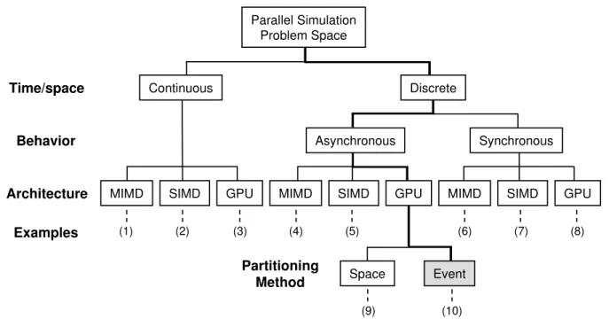
3.4 Parallel Simulation Problem Space
Parallel simulation problem space can be classified using time-space and classes of parallel computers, as shown in Figure3-1. Parallel simulation models fall into two
Continuous Discrete Asynchronous Synchronous MIMD Parallel Simulation Problem Space SIMD GPU
MIMD SIMD GPU MIMD SIMD GPU
Space Event (1) (10) (9) (5) (6) (2) (3) (4) (7) (8) Time/space Behavior Architecture Examples Partitioning Method
Figure 3-1. Diagram of parallel simulation problem space Table 3-1. Classification of parallel simulation examples
Index Examples
(1) Ordinary differential equations [62] (2) Reservoir simulation [63]
(3) Cloud dynamics [47], N-body simulation [48] (4) Chandy and Misra [25], Time-warp [29] (5) Ayani and Bourkman [44], Shu and Wu [45] (6) Partial differential equations [64]
(7) Cellular automata [65] (8) Retina simulation [46]
(9) Diffusion simulation [49], Xu and Bagrodia [50] (10) Our queuing model simulation
major categories: continuous and discrete. Most physical simulations are continuous simulations (i.e., ordinary and partial differential equations, cellular automata); however, complex human-made systems (i.e., communication networks) tend to have a discrete structure. Discrete models can be categorized into two, in regards to the behavior of simulation models: asynchronous (discrete-event) and synchronous (time-stepped) models. Asynchronous models can be classified according to how the partitioning is done. The examples of each branch in Figure3-1are summarized in Table3-1.
CHAPTER 4
A GPU-BASED APPLICATION FRAMEWORK SUPPORTING FAST DISCRETE EVENT SIMULATION
4.1 Parallel Event Scheduling
SIMD-based computation has a bottleneck problem in that some operations, such as instruction fetch, have to be implemented sequentially, which causes many processors to be halted. Event scheduling in SIMD-based simulation can be considered as a step of instruction fetch that distributes the workload into each processor. The sequential operations in a shared event list can be crucial to the overall performance of simulation for a large-scale model. Most implementations of concurrent priority queue have been run on MIMD machines. Their asynchronous operations reduce the number of locks at the instant time of simulation. However, it is inefficient to implement a concurrent priority queue with a lock-based approach on SIMD hardware, especially a GPU because the point in time when multiple threads access the priority queue is synchronized. It produces many locks that are involved in mutual exclusion, making their operations almost sequential. Moreover, sparse and dynamic data structure, such as heaps, cannot be directly developed on the GPU since the GPU is optimized to process dense and static data structures such as linear arrays.
Both insert and delete-min operations re-sort the FEL in timestamp order. Other threads cannot access the FEL during the sort, since all the elements in the FEL are sorted if a linear array is used for the data structure of the FEL. The concept of parallel event scheduling is that an FEL is divided into many sub-FELs, and only one of them is handled by each thread on the GPU. An element index that is used to access the element in the FEL is calculated by a thread ID combined with a block ID, which allows each thread to access its elements in parallel without any interference from other threads. In addition, keeping the global FEL unsorted guarantees that each thread can access its elements, regardless of the operations of other threads. The number of
while(current time is less than simulation time) // executed by multiple threads
minimumTimestamp = ParallelReduction(FEL);
foreach local FEL by each thread in parallel do
currentEvent = ExtractEvent(minimumTimestamp); nextEvent = ExecuteEvent(currentEvent);
ScheduleEvent(nextEvent);
end for each end while
Figure 4-1. The algorithm for parallel event scheduling
elements that each thread is responsible for processing at the current time is calculated by dividing the number of elements in the FEL by the number of threads.
As a result, the heads of the global FEL and each local FEL accessed by each thread are not the events with the minimum timestamp. Instead, the smallest timestamp is determined by parallel reduction [14,66], using multiple threads. With this timestamp, each thread compares the minimum timestamp with that of each element in the local FEL to find and extract the current active events (delete-min). After the current events are executed in parallel, new events are created by the current events. The currently extracted elements in the FEL are re-written by updating the attributes, such as an event and its time (insert). The algorithm for parallel event scheduling on the GPU is summarized in Figure4-1.
Additional operations are needed for a queuing model simulation. The purpose of discrete event simulation is to analyze the behavior of the system [67]. In a queuing model simulation, a service facility is the system to be analyzed. Service facilities are modeled in arrays as resources that contain information regarding server status, current customers, and their queues. Scheduling the incoming customer to the service facility (Arrival), releasing the customer after its service (Departure), and manipulating the queue when its server is busy are the service facility operations. Queuing model simulations also benefit from the tens of thousands of threads on the GPU. However,
there are some issues to be considered, since the arrays of both the FEL and service facility reside in global memory, and threads share them.
4.2 Issues in a Queuing Model Simulation
4.2.1 Mutual Exclusion
Most simulations that are run on a GPU use 2D or 3D spaces to represent the simulation results. The spaces and the variables, used for updating those spaces, are implemented in an array on the GPU. The result array is updated based on variable arrays throughout the simulation. For example, the velocity array is used for updating the result array by a partial differential equation in a fluid simulation. The result array is dependent on the variable arrays, but not vice versa. In a fluid simulation, the changes of velocity in a fluid simulation make the result different, but the result array does not change the velocity. This kind of update is one-directional. Mutual exclusion is not necessary, since each thread is responsible for a fixed number of elements, and does not interfere with other threads.
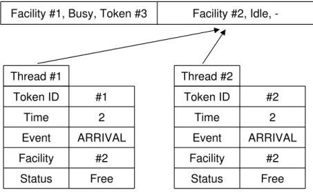
However, the updates in a queuing model simulation are bi-directional. One event simultaneously updates both the FEL and service facility arrays. Bi-directional updates occurring at the same time may cause their results to be incorrect, because one of the element indexes–either the FEL or the service facility–cannot be accessed by other threads independently. For example, consider a concurrent request to the same service facility that has only one server, as shown in Figure4-2A. Both threads try to schedule their token to the server because its idle status is read by both threads at the same time. The simultaneous writing to the same location leads to the wrong result in thread #1, as shown in Figure4-2B. We need a mutual exclusion algorithm because data inconsistency can occur when updating both arrays at the same time. The mutual exclusion involved in this environment is different from the case of the concurrent priority queue, in that two different arrays concurrently attempt to update each other and are accessed by the same element index.
Facility #1, Busy, Token #3 Facility #2, Idle, -Token ID #1 Time 2 Event ARRIVAL Facility #2 Status Free Thread #1 Token ID #2 Time 2 Event ARRIVAL Facility #2 Status Free Thread #2
A A concurrent request from two threads
Facility #1, Busy, Token #3 Facility #2, Busy, Token #2
Token ID #1 Time 2 Event ARRIVAL Facility #2 Status Served Thread #1 Token ID #2 Time 2 Event ARRIVAL Facility #2 Status Served Thread #2
B The incorrect results for a concurrent request. The status of token #1 should be Queue.
Figure 4-2. The result of a concurrent request from two threads without a mutual exclusion algorithm
The simplest way to implement mutual exclusion is to separate both updates. Alternate access between the FEL and service facility can resolve this problem. When updates are happening in terms of the FEL, each extracted token in the FEL stores information about the service facility, indicating that an update is required at the next step. Service facilities are then updated based on these results. Each service facility searches the FEL to find the extracted tokens that are related to itself at the current time.