HEC-SSP
Statistical Software Package
User’s Manual
Version 2.0
The public reporting burden for this collection of information is estimated to average 1 hour per response, including the time for reviewing instructions, searching existing data sources, gathering and maintaining the data needed, and completing and reviewing the collection of information. Send comments regarding this burden estimate or any other aspect of this collection of information, including suggestions for reducing this burden, to the Department of Defense, Executive Services and Communications Directorate (0704-0188). Respondents should be aware that notwithstanding any other provision of law, no person shall be subject to any penalty for failing to comply with a collection of information if it does not display a currently valid OMB control number.
PLEASE DO NOT RETURN YOUR FORM TO THE ABOVE ORGANIZATION. 1. REPORT DATE (DD-MM-YYYY)
October 2010
2. REPORT TYPE
Computer Program Documentation
3. DATES COVERED (From - To)
4. TITLE AND SUBTITLE
HEC-SSP
Statistical Software Package Version 2.0
5a. CONTRACT NUMBER
5b. GRANT NUMBER
5c. PROGRAM ELEMENT NUMBER
6. AUTHOR(S)
Gary W. Brunner and Matthew J. Fleming
5d. PROJECT NUMBER
5e. TASK NUMBER
5F. WORK UNIT NUMBER
7. PERFORMING ORGANIZATION NAME(S) AND ADDRESS(ES)
US Army Corps of Engineers Institute for Water Resources
Hydrologic Engineering Center (HEC) 609 Second Street
Davis, CA 95616-4687
8. PERFORMING ORGANIZATION REPORT NUMBER
CPD-86
9. SPONSORING/MONITORING AGENCY NAME(S) AND ADDRESS(ES) 10. SPONSOR/ MONITOR'S ACRONYM(S) 11. SPONSOR/ MONITOR'S REPORT NUMBER(S) 12. DISTRIBUTION / AVAILABILITY STATEMENT
Approved for public release; distribution is unlimited.
13. SUPPLEMENTARY NOTES
14. ABSTRACT
The Hydrologic Engineering Center's Statistical Software Package (HEC-SSP) allows the user to perform statistical analyses of hydrologic data. The current version of HEC-SSP can perform flood flow frequency analysis based on Bulletin 17B, a general frequency analysis using any type of hydrologic data, a volume frequency analysis, a duration analysis, a coincident frequency analysis, and a curve combination analysis. Data storage and management is handled either through the use of text files (ASCII, XML), as well as the Hydrologic Engineering Center's Data Storage System (HEC-DSS).
15. SUBJECT TERMS
HEC-SSP, flood frequency, statistics, Bulletin 17B, flow, stage, computer program, hydrologic data, volume-duration, statistical analysis, data storage, reporting tools, frequency curves, confidence limits, low outliers, high outliers, regional skews
16. SECURITY CLASSIFICATION OF: 17. LIMITATION OF ABSTRACT UU 18. NUMBER OF PAGES 313
19a. NAME OF RESPONSIBLE PERSON a. REPORT U b. ABSTRACT U c. THIS PAGE U 19b. TELEPHONE NUMBER
HEC-SSP
Statistical Software Package
User’s Manual
October 2010
US Army Corps of Engineers
Institute for Water Resources
Hydrologic Engineering Center
609 Second Street
Statistical Software Package, HEC-SSP Software Distribution and Availability Statement
The HEC-SSP executable code and documentation are public domain and were developed by the Hydrologic Engineering Center for the U.S. Army Corps of Engineers. The software was developed with United States Federal Government resources, and is therefore in the public domain. This software can be downloaded for free from the HEC internet site
(www.hec.usace.army.mil). HEC does not provide technical support for this software to non-Corps users. However, we will respond to all documented instances of program errors. Documented errors are bugs in the software due to programming mistakes not model problems due to user-entered data.
Table of Contents
CHAPTER 1 ... 1-1 Introduction ... 1-1 Contents ... 1-1 General Philosophy of the HEC-SSP ... 1-2 Overview of Program Capabilities ... 1-2 User Interface ... 1-2 Statistical Analysis Components ... 1-3 Data Storage and Management ... 1-3 Graphical and Tabular Output ... 1-4 Overview of This Manual ... 1-4 CHAPTER 2 ... 2-1 Installing HEC-SSP ... 2-1 Contents ... 2-1 Hardware and Software Requirements ... 2-2 Installation Procedure ... 2-2 To install the software onto your hard disk do the following: ... 2-2 Uninstall Procedure ... 2-3 CHAPTER 3 ... 3-1 Working With HEC-SSP - An Overview ... 3-1 Contents ... 3-1 Starting HEC-SSP ... 3-2 To Start HEC-SSP from Windows: ... 3-2 Overview of the Software Layout ... 3-2 Steps in Performing a Bulletin 17B Frequency Analysis ...3-10 Starting a New Study ... 3-10 Adding a Background Map ... 3-11 Importing, Entering, and Editing Data ... 3-13 Performing the Bulletin 17B Flow Frequency Analysis ... 3-17 Viewing and Printing Results ... 3-18 CHAPTER 4 ... 4-1 Using the HEC-SSP Data Importer ... 4-1 Contents ... 4-1 Developing a New Data Set ... 4-2 Importing Data from an HEC-DSS File ... 4-3 Importing Data from the USGS Website ... 4-4 Importing Data from an Excel Spreadsheet ... 4-7 Entering Data Manually ... 4-10 Importing Data from a Text File ... 4-11 Metadata ...4-15 Plotting and Tabulating the Data ...4-17 CHAPTER 5 ... 5-1 Performing a Bulletin 17B Flow Frequency Analysis ... 5-1 Contents ... 5-1 Starting a New Analysis ... 5-2 General Settings, Options, and Computations ... 5-3
Plotting Positions ... 5-4 Confidence Limits ... 5-5 Time Window Modification ... 5-5 Options ... 5-5 Low Outlier Threshold... 5-6 Historic Period Data ... 5-7 User Specified Frequency Ordinates ... 5-8 Compute ... 5-8 Viewing and Printing Results ... 5-8 Tabular Output ... 5-9 Graphical Output ... 5-10 Viewing the Report File ... 5-12 CHAPTER 6 ... 6-1 Performing a General Frequency Analysis ... 6-1 Contents ... 6-1 Starting a New Analysis ... 6-2 General Settings and Options ... 6-3 General Settings ... 6-3 Log Transform ... 6-3 Plotting Positions ... 6-4 Confidence Limits ... 6-4 Time Window Modification ... 6-5 Options ... 6-5 Low Outlier Threshold... 6-6 Historic Period Data ... 6-7 User Specified Frequency Ordinates ... 6-8 Output Labeling ... 6-8 Analytical Frequency Analysis ... 6-8 Settings ... 6-9 Distribution ... 6-10 Generalized Skew ... 6-10 Expected Probability Curve ... 6-11 Compute ... 6-11 Tabular Results ... 6-11 Plot ... 6-13 Graphical Frequency Analysis ... 6-15 Viewing and Printing Results ... 6-16 Tabular Output ... 6-16 Graphical Output ... 6-17 Viewing the Report File ... 6-19 CHAPTER 7 ... 7-1 Performing a Volume Frequency Analysis ... 7-1 Contents ... 7-1 Starting a New Volume Frequency Analysis ... 7-2 General Settings and Options ... 7-3 General Settings ... 7-3 Log Transform ... 7-3 Plotting Positions ... 7-4 Maximum or Minimum Analysis ... 7-5 Year Specification ... 7-5 Time Window Modification ... 7-6 Options ... 7-7 Flow-Durations ... 7-8 User Specified Frequency Ordinates ... 7-9
Output Labeling ... 7-9 Low Outlier Threshold ... 7-10 Historic Period Data ... 7-10 Extracting The Volume-Duration Data ...7-12 Analytical Frequency Analysis ...7-14 Settings ... 7-15 Distribution ... 7-15 Expected Probability Curve ... 7-16 Skew ... 7-16 Compute ...7-17 Tabular Results ... 7-17 Plot ... 7-18 Statistics ... 7-19 Graphical Frequency Analysis ...7-20 Curve Input ... 7-21 Plot ... 7-21 Viewing and Printing Results – Volume Frequency Analysis ...7-22 Tabular Output ... 7-22 Graphical Output ... 7-23 Viewing the Report File ... 7-24 CHAPTER 8 ... 8-1 Performing a Duration Analysis ... 8-1 Contents ... 8-1 Starting a New Analysis ... 8-2 General Settings and Options ... 8-3 General ... 8-3 Method ... 8-3 X-Axis Scale ... 8-3 Y-Axis Scale ... 8-4 Time Window Modification ... 8-4 Duration Period ... 8-4 Options ... 8-5 Output Labeling ... 8-6 Plotting Position Formula ... 8-6 User-Specified Exceedance Ordinates ... 8-7 Bin Limits ... 8-7 Compute ... 8-8 Results ... 8-9 Tabular Results ... 8-9 Plot ... 8-10 Manual Duration Analysis ... 8-11 Viewing and Printing Results ...8-12 Tabular Output ... 8-12 Graphical Output ... 8-13 Viewing the Report File ... 8-14 CHAPTER 9 ... 9-1 Performing a Coincident Frequency Analysis ... 9-1 Contents ... 9-4 Starting a New Analysis ... 9-4 General Settings ... 9-5 Variable A ... 9-5
Y-Axis Scale ... 9-6 User Specified Frequency Ordinates ... 9-6 Variable A ... 9-7 Variable B ... 9-8 Response Curves ... 9-11 Compute ... 9-14 Results ... 9-15 Viewing and Printing Results ... 9-16 Tabular Output ... 9-16 Graphical Output ... 9-16 Viewing the Report File ... 9-18 CHAPTER 10 ... 10-1 Performing a Curve Combination Analysis ... 10-1 Contents ... 10-2 Starting a New Analysis ... 10-2 General Settings ... 10-3 Number of Curves ... 10-3 Output Labeling ... 10-3 Data Type ... 10-4 Y-Axis Scale ... 10-4 Confidence Limits Method ... 10-4 Frequency of PMF ... 10-5 Confidence Limits ... 10-6 User Specified Frequency Ordinates ... 10-7 Frequency Curves... 10-7 Confidence Limits ... 10-9 Compute ... 10-12 Results ... 10-12 Viewing and Printing Results ... 10-13 Tabular Output ... 10-13 Graphical Output ... 10-13 Viewing the Report File ... 10-15 References ... A-1 Example Data Sets ... B-1 Example 1: Fitting the Log-Pearson Type III Distribution ... B-4 Example 2: Analysis with High Outliers ... B-12 Example 3: Testing and Adjusting for a Low Outlier ... B-20 Example 4: Zero-Flood Years ... B-28 Example 5: Confidence Limits and Low Threshold Discharge ... B-36 Example 6: Use of Historic Data and Median Plotting Position ... B-44 Example 7: Analyzing Stage Data ... B-52 Example 8: Using User-Adjusted Statistics ... B-59 Example 9: General Frequency – Graphical Analysis ... B-69 Example 10: Volume Frequency Analysis, Maximum Flows ... B-76 Example 11: Volume Frequency Analysis, Minimum Flows ... B-87 Example 12: Duration Analysis, BIN (STATS) Method ... B-98 Example 13: Duration Analysis, Rank All Data Method ... B-104 Example 14: Duration Analysis, Manual Entry ... B-110 Example 15: Coincident Frequency Analysis, A and B can be Assumed Independent ... B-113 Example 16: Coincident Frequency Analysis, A and B can not be Assumed IndependentB-120 Example 17: Curve Combination Analysis, Combine Flow Frequency Curves ... B-127 Example 18: Curve Combination Analysis, Combine Stage Frequency Curves ... B-132
Foreword
The U.S. Army Corps of Engineers’ Statistical Software Package (HEC-SSP) is software that allows you to perform statistical analyses of hydrologic data.
The first official version of HEC-SSP (version 1.0) was released in August of 2008. Version 1.1 was released in April, 2009 and included improvements to data entry, results visualization and reporting, and added capability to the volume frequency analysis. These new features are discussed in the User’s Manual and in the release notes for Version 1.1. Version 2.0 was released in October 2010 and included three new analyses: a duration analysis, a coincident frequency analysis, and a curve combination analysis. These new features are discussed in the User’s Manual and in the release notes for Version 2.0.
The HEC-SSP software was designed by Mr. Gary Brunner, Mr. Jeff Harris, Dr. Beth Faber, and Mr. Matthew Fleming. The HEC-SSP user interface was programmed by Mr. Mark Ackerman, and the
computational code was programmed by Mr. Paul Ely. This manual was written by Mr. Gary Brunner and Mr. Matthew Fleming.
C H A P T E R 1
Introduction
Welcome to the U.S. Army Corps of Engineers Statistical Software Package (HEC-SSP) developed by the Hydrologic Engineering Center. This software allows you to perform statistical analyses of hydrologic data. The current version of HEC-SSP can perform flood flow
frequency analysis based on Bulletin 17B, "Guidelines for Determining Flood Flow Frequency" (1982), a generalized frequency analysis on not only flow data but other hydrologic data as well, a volume frequency analysis on high and low flows, a duration analysis, a coincident frequency analysis, and a curve combination analysis.
The HEC-SSP software system was developed as a part of the Hydrologic Engineering Center's "Next Generation" (NexGen)
development of hydrologic engineering software. The NexGen project encompasses several aspects of hydrologic engineering, including rainfall-runoff analysis, river hydraulics, reservoir system simulation, flood damage analysis, and real-time river forecasting for reservoir operations.
This chapter discusses the general philosophy of HEC-SSP and gives a brief overview of the capabilities of the software system. An overview of this manual is also provided.
Contents
• General Philosophy of the HEC-SSP
• Overview of Program Capabilities
General Philosophy of the HEC-SSP
HEC-SSP is an integrated system of software, designed for interactive use in a multi-tasking environment. The system is comprised of a graphical user interface (GUI), separate statistical analysis
components, data storage and management capabilities, mapping, graphics, and reporting tools.
Over a period of many years, the Hydrologic Engineering Center has supported a variety of statistical packages that perform frequency analysis and other statistical computations. Historically, the programs that received the most use within the Corps of Engineers were HEC-FFA (Flood Frequency Analysis) and STATS (Statistical Analysis of Time Series Data). FFA incorporates Bulletin 17B procedures that have been adopted by the Corps for flow frequency analysis. The STATS software package is used for statistical analysis of time series data. STATS can provide either analytical or graphical frequency analysis, specified by the user. STATS has the capability of computing monthly and annual maximum, minimum, and mean values along with
computing a volume-duration analysis. Two other packages that have received a lot of use within the Corps of Engineers are REGFRQ
(Regional Frequency Computation) and MLRP (Multiple Linear
Regression Program). REGFRQ performs regional frequency analysis and MLRP is a multiple linear regression analysis tool.
The goal of HEC-SSP is to ultimately combine all of the statistical analyses capabilities of HEC-FFA, STATS, REGFRQ and MLRP. The current version of HEC-SSP supports performing flood flow frequency analyses based on Bulletin 17B Guidelines, general frequency
analyses, volume frequency analyses, duration analyses, coincident frequency analyses, and curve combination analyses. New features and additional capabilities will be added in future releases.
Overview of Program Capabilities
HEC-SSP is designed to perform statistical analyses of hydrologic data. The following is a description of the major capabilities of HEC-SSP.
User Interface
The user interacts with HEC-SSP through a graphical user interface (GUI). The main focus in the design of the interface was to make it easy to use the software, while still maintaining a high level of efficiency for the user. The interface provides for the following functions:
• File management
• Data entry, importing, and editing
• Statistical analyses
• Tabulation and graphical displays of results
• Reporting facilities
Statistical Analysis Components
Flow Frequency Analysis (Bulletin 17B) – This component of the
software allows the user to perform annual peak flow frequency analyses. The software implements procedures in Bulletin 17B,
"Guidelines for Determining Flood Flow Frequency", by the Interagency Advisory Committee on Water Data.
General Frequency Analysis – This component of the software allows
the user to perform annual peak flow frequency analyses by various methods. Additionally the user can perform frequency analysis of variables other than peak flows, such as stage and precipitation data.
Volume Frequency Analysis – This component of the software allows
the user to perform a volume frequency analyses on daily flow or stage data.
Duration Analysis – This component of the software allows the user to
perform a duration analysis on any type of data recorded at regular intervals. The duration analysis can be used to show the percent of time that a hydrologic variable is likely to equal or exceed some specific value of interest.
Coincident Frequency Analysis – This component of the software
assists the user in computing the exceedance frequency relationship for a variable that is a function of two other variables.
Curve Combination Analysis
Data Storage and Management
– This component provides a tool for combining frequency curves from multiple sources into one frequency curve.
Data storage is accomplished through the use of "text" files (ASCII and XML), as well as the HEC Data Storage System (HEC-DSS). User input data are stored in flat files under separate categories of study,
analyses, and a data storage list. Gage data are stored in a project HEC-DSS file as time series data. Output data is predominantly stored in HEC-DSS, while a summary of the results is written to an XML file. Additionally, an analysis report file is generated whenever a
Data management is accomplished through the user interface. The modeler is requested to enter a Name and Description for each study being developed. Once the study name is entered, a directory with that name is created, as well as a study file. Additionally, a set of subdirectories is created with the following names: Bulletin17bResults, GeneralFrequencyResults, VolumeFrequencyAnalysisResults,
DurationAnalysisResults, CoicidentFreqResults,
CurveCombinationAnalysis, Layouts, and Maps. As the user creates new analyses, an analysis file is created in the main project directory. The interface provides for renaming and deletion of files on a study-by-study basis.
Graphical and Tabular Output
Graphics include a map window, plots of the data, and plots of analysis results. The map window can be used to display background map layers. Locations of the data being analyzed can be displayed on top of the map layers. Once data are brought into HEC-SSP, they can be plotted for visual inspection. The frequency curve plots show the results of the analyses, which include the analytically computed curve, the expected probability curve, confidence limits, and the raw data points plotted based on the selected plotting position method. Tabular output consists of tables showing the computed frequency curves, confidence limits, and summary statistics. All graphical and tabular output can be displayed on the screen, sent directly to a printer (or plotter), or passed through the Windows Clipboard to other software, such as a word-processor or spreadsheet.
A report file is available for each analysis. This report file includes the input data, preliminary results, all of the statistical tests (Low and High Outliers, Broken Record, Zero Flows Years, Incomplete Record,
Regional Skews, and Historic Information), and final results. This report file is similar to the FFA output file.
Overview of This Manual
This user's manual is the primary documentation on how to use HEC-SSP. The manual is organized as follows:
• Chapters 1-2 provide an introduction and overview of HEC-SSP, as well as instructions on how to install the software.
• Chapter 3 provides an overview on how to use the HEC-SSP
software in a step-by-step procedure, including a sample problem that the user can follow.
• Chapter 4 explains in detail how to enter and view data.
• Chapter 5 provides a detailed discussion on how to perform the Bulletin 17B flow frequency analysis. Additionally, this chapter describes all of the output capabilities available for displaying and printing the results.
• Chapter 6 provides a detailed discussion on how to use the general frequency analysis editor.
• Chapter 7 provides a detailed discussion on how to use the volume frequency analysis editor.
• Chapter 8 provides a detailed discussion on how to use the duration analysis editor.
• Chapter 9 provides a detailed discussion on how to use the coincident frequency analysis editor.
• Chapter 10 provides a detailed discussion on how to use the curve combination analysis editor.
• Appendix A contains a list of references.
• Appendix B has a series of example analyses that demonstrate the various capabilities of performing a Bulletin 17B flow frequency analysis, a general frequency analysis, a volume-duration frequency analysis, a volume-duration analysis, a coincident frequency analysis, and a curve combination analysis.
C H A P T E R 2
Installing HEC-SSP
You install HEC-SSP using the program installation package available from HEC’s web site. The setup program installs the software,
documentation, and the example applications. This chapter discusses the hardware and system requirements needed to use HEC-SSP, how to install the software, and how to uninstall the software.
Contents
• Hardware and Software Requirements
• Installation Procedure
Hardware and Software Requirements
Before you install the HEC-SSP software, make sure that your
computer has at least the minimum required hardware and software. In order to get the maximum performance from the HEC-SSP
software, recommended hardware and software is shown in
parentheses. This version of HEC-SSP will run on a computer that has the following:
• Intel Based PC or compatible machine with Pentium processor or higher (a Pentium 4 or higher is recommended).
• A hard disk with at least 100 megabytes of free space
• A CD-Rom drive (or CD-R, CD-RW, DVD), if installing from a CD.
• A minimum of 512 megabytes of RAM (1 Gigabyte or more is
recommended).
• A mouse.
• Color Video Display (Recommend running in 1280x1024 or higher
resolution, and as large a monitor as possible). Recommend at least a 17" monitor.
• Microsoft Windows NT 4.0, 2000, XP, or Vista (or later versions).
Installation Procedure
Installation of the HEC-SSP software is accomplished through the use of the Setup program.
To install the software onto your hard disk do the
following:
1.Insert the HEC-SSP CD into your CD drive (or download the software from our web site: www.hec.usace.army.mil).
2. The setup program should run automatically if installing from a CD. When downloading from the web page you will need to save the setup file in a temporary directory and then execute the “HEC-SSP_2_Setup.exe” file to run the setup program.
3. If the setup program does not automatically run from the CD, use the windows explorer to start the HEC-SSP_2_Setup.exe program on the CD.
The setup program automatically creates a program group called HEC. This program group will be listed under the Programs menu, which is under the Start menu. The HEC-SSP program icon will be contained within the HEC program group, within the HEC-SSP subdirectory. The user can request that a shortcut icon for HEC-SSP be created on the desktop. If installed in the default directory, the HEC-SSP executable can be found in the C:\Program Files\HEC\HEC-SSP\2.0 directory with the name "HEC-SSP.EXE".
The HEC-SSP User’s Manual and example data sets are also installed with the software. The User’s Manual can be viewed by selecting
User’s Manual from the Help menu. You must have Adobe Acrobat
Reader to view the user’s manual. This viewer can be obtained for free from the Adobe web page.
A zip file containing the example data sets described in Appendix B have been installed in the "…\Examples" folder within the program directory. You can install the example data sets by selecting the
Install Example Data option from the Help menu. After selecting
the Install Example Data menu option, a window will open for you to choose a location to install the example data sets. The program will create a subdirectory within your chosen folder called SSP_Examples. A project file called "SSP_EXAMPLES.ssp" will be contained in the
SSP_Examples folder. You can load the test data sets by using the
Open Study option from the File menu and then use the file chooser
to select this file.
Uninstall Procedure
The HEC-SSP Setup program automatically registers the software with the Windows operating system. To uninstall the software, do the following:
• From the Start Menu select Control Panel.
• Select Add/Remove Programs from within the Control Panel folder.
• From the list of installed software, select the HEC-SSP program and press the Remove button.
• Follow the uninstall directions on the screen and the software will be removed from your hard disk.
C H A P T E R 3
Working With HEC-SSP - An Overview
HEC-SSP is an integrated package of statistical analysis modules, in which the user interacts with the system through the use of a Graphical User Interface (GUI). The current version is capable of performing flow frequency analyses based on Bulletin 17B "Guidelines for Determining Flood Flow Frequency", dated March 1982, general frequency analyses, volume frequency analyses, duration analyses, coincident frequency analyses, and curve combination analyses. This chapter provides an overview of how a Bulletin 17B flow frequency analyses can be performed with the HEC-SSP software. General frequency and volume-duration frequency analyses can be developed in a similar manner as outlined for the Bulletin 17B analysis.
In HEC-SSP terminology, a Study is a set of files associated with a particular set of data and statistical analyses being performed. The files for a study are categorized as follows: study information, data list, and analysis data.
Contents
• Starting HEC-SSP
• Overview of the Software Layout
Starting HEC-SSP
When you run the HEC-SSP Setup program, a new program group called HEC and a program icon called HEC-SSP are created. They should appear in the start menu under the section called All
Programs. The user also has the option of creating a shortcut on the
desktop. If a shortcut is created, the icon for HEC-SSP will look like the following:
Figure 3-1. The HEC-SSP Icon.
To Start HEC-SSP from Windows:
• Double-click on the SSP Icon. If you do not have an HEC-SSP shortcut on the desktop, go to the Start menu and select All
Programs HEC HEC-SSP HEC-SSP 2.0.
Overview of the Software Layout
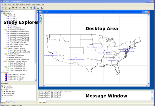
When you first start HEC-SSP, you will see the main window as shown in Figure 3-2, except you will not have any study data on your main window. As shown in Figure 3-2, the main window is laid out with a Menu Bar, a Tool Bar, and four window panes.
The upper right pane (which occupies most of the window area) is the
Desktop Area (Referred to as the "Desktop" from this point in the
manual). This area is used for displaying maps, data editors, and analysis windows.
The upper left pane is called the Study Explorer. The Study Explorer acts like an explorer tree for the study. The top level of the tree is the study (SSP Examples in this example). Below the study is an analysis branch, a data branch, and a map branch. Under the analysis branch, the first level is the type of analysis. Under each analysis type will be the current user-defined analyses for that type. The data branch lists all of the available data sets that have been brought into the current study. Generally, a data set represents a piece of data at a specific gage location. For example, all of the peak annual flows at a single gage would be stored as a single data set. When an analysis is created, the user selects a data set to be used for that particular analysis. The map branch of the tree contains any maps the user has put together for the study. By default there is automatically a "Base Map" listed under the maps folder.
The lower left pane, and associated tabs, also belongs to the study explorer. This window is used to show additional information about items selected in the study explorer. The tabs are used to switch to different views within the study explorer window. The first tab, labeled Study, shows the explorer view of the study. The second tab, labeled Maps, lists the available maps and map layers associated with each map. The last tab, labeled Files, shows all of the files that make up the current study.
The lower right pane is called the Message Window. This window is used to display messages from the software as to what it is doing.
Figure 3-2. The HEC-SSP Main Window.
Study Explorer
Desktop Area
At the top of the HEC-SSP main window is a Menu bar with the following options:
File: This menu is used for file management. Options available under
the File menu include New Study, Open Study, Save Study, Save Study As, Close Study, Study Properties, Export, Recent Studies, and Exit. The Study Properties option is used to describe the study and to set the units system. The Export option is used to export HEC-SSP results, stored in the study DSS file, to another DSS file. The Recent Studies option lists the most recently opened studies, which allows the user to quickly open a study that was recently worked on.
Edit: This menu is used for applying the Cut, Copy, and Paste
clipboard features to data in editable fields and tables.
View: The View menu allows the user to control display of the
toolbars and the study windows. The user can also toggle between viewing all of the panes or just the Main View Pane. The View menu also has options for saving the current layout (currently opened windows and their sizes and locations) and restoring a previously saved layout. The Set Study Display Units option allows the user to switch output between English and metric units. The Select Working Sets menu option allows the user to group items in each folder and then display only those items in the user interface. For example, Figure 3-3 shows the Bulletin 17B folder in the study explorer. The Edit Working Set editor, Figure 3-4, was used to group all Bulletin 17B analyses that started with “FFA” into one working set. The working set
was named “FFA Analyses”. This working set was activated by right clicking on top of the Bulletin 17B folder in the study explorer and selecting Select Working SetsFFA Analyses, as shown in Figure
3-5. Only the Bulletin 17B analyses within the working set will then be displayed in the study explorer, as shown in Figure 3-6. To display all Bulletin 17B analysis, right click on top of the Bulletin 17B folder in the
study explorer and select Select Working SetsNo Working Set.
Figure 3-3. Study Explorer before Defining a Working Set.
Figure 3-5. Activate a Working Set from the Study Explorer.
Figure 3-6. Bulletin 17B Folder Only Displays Analyses in Working Set.
Maps: This menu is used to set the Default Map Properties
(Coordinate system, extents, etc…), define a new map, add map layers to the study, and remove a map. Additionally, this menu has the following options available: Map Window Settings (allows the user to turn map layers on and off), Zoom To Entire Map Extents, Save Map Image, Import, and Export. The Zoom To Entire Map Extents option displays the entire set of map layers within the map window. The Save Map Image option can be used to save the current view of the map to a file.
Data: This menu allows the user to define a new data set, open the
metadata editor, and delete any existing data sets from the data list. Other options include opening a plot and table of the data.
Analysis: This menu is used to create the various statistical analyses
available in the software. Each statistical analysis is saved as a separate file
containing the information that is pertinent to that specific analysis type. The current options under this menu item include New, Open, Delete from Study, Save, Save As, Rename, and Compute Manager. The compute manager allows the user to select one, several, or all of the analyses, and then have them all recomputed.
Results: This menu allows the user to graph and tabulate any of the
existing analyses that have been computed. Additionally, the user can request to view the report file from a analysis. Users must select at least one analysis in the Study Explorer before selecting Graph, Table, Report, or Summary Report. If more than one analysis of the same type are selected (this is
accomplished by holding down the control key while clicking on the various analyses), the Graph and Summary Report options will include results from all analyses that are selected. However, when multiple analyses are selected, the Table and Report option bring up separate windows for each of the selected analyses. The Default Plot Line Styles menu option lets the user change the default line styles applied to different data types that are plotted in a graph. For example, the user can
Tools: This menu includes HEC-DSSVue, Plot Probability Lines,
Options, Console Output, and Memory Monitor. The HEC-DSSVue option brings up the HEC-DSSVue program and automatically loads the current study DSS file. HEC-DSSVue is a DSS utility to tabulate, graph, edit, and enter data into DSS. The Plot Probability Lines option opens an editor, shown in Figure 3-7, that lets the user add, delete, or edit the probability lines and axis labels that are displayed in all frequency curve plots. The Options menu item opens the Options editor that allows the user to set default HEC-SSP options. The Results tab in the Options editor, shown in Figure 3-8, allows the user to set the number of decimal digits that are displayed in all results.
Figure 3-8. Dialog for Controlling the Number of Decimal Digits Shown in Result Tables and Reports.
Window: This menu includes Tile, Cascade, Next Window, Previous
Window, Window Selector, and Window. These options are used to control the appearance of the windows in the Desktop area. When more than one window is open (such as a data importer, and various analysis windows), these menu items will help the user organize the windows, or quickly navigate to a specific window. The Tile option can be used to organize all of the currently opened windows in either a vertical or horizontal tile. The Cascade option puts one window on top of the next in a cascading fashion. The Next Window option brings the next window in the list of currently opened windows to the top. The Previous Window brings the last window that was on top back to the top. The Window Selector option brings up a pick list of the currently opened windows and allows you to select the one you want. The Window option has a sub menu list of all the opened windows and allows you to select one.
Help: This menu allows the user to open the HEC-SSP User’s Manual,
install example data sets, read the terms and conditions of use statement, and display the current version information about
HEC-SSP.
Also on the HEC-SSP main window is a Tool Bar. The buttons on the tool bar provide quick access to the most frequently used options under the HEC-SSP File and Edit menus.
Steps in Performing a Bulletin 17B Frequency Analysis
There are five main steps in performing a Bulletin 17B flow frequency analysis using HEC-SSP. Similar steps are required when performing other statistical analyses.
• Starting a new study
• Adding a Background Map (Optional)
• Importing, Entering, and Editing Data
• Performing the Bulletin 17B Frequency Analysis
• Viewing and Printing Results
Starting a New Study
The first step in performing a Flow Frequency analysis with HEC-SSP is to establish which directory you wish to work in and to enter a title for the new study. To start a new study, go to the File menu and select
New Study. This will open the Create New Study window as shown
in Figure 3-9. The user is required to enter a name for the study, select a directory to work in (a default location is provided), and select the desired units system. Adding a description of the study is optional. Once you have entered all the information, press the OK button to have the information accepted. After the OK button is pressed, a subdirectory will be created under the user chosen directory. The subdirectory will be labeled with the same name as the user-entered study name. This study directory is where the HEC-SSP project file, as well as other study files and directories will be located. Additionally, a default map window will appear in the Main View Pane. However, the map window will be blank when it first opens.
Figure 3-9. New Study Window.
Adding a Background Map
By default, when you start a new project in HEC-SSP a default map window (called Base Map) will open in the Desktop window. Having a background map is optional in HEC-SSP. Not having a map does not prevent the user from importing and entering data, or performing an analysis and viewing results. The map is mostly a visual aid of the study area. Additionally, when you bring in gage data you can enter the map coordinates of the gage and it will show up on the map. Once a gage is located on the map you can right click on it to open a
shortcut menu for viewing the data, or graphing and tabulating the results.
To add a map layer to the default map, go to the Maps menu and select Add Map Layers. When this option is selected a file chooser window will appear, as shown in Figure 3-10, allowing the user to select map layers to bring into the map. The Create Copy option on the window will make a copy of the selected map and place it in the Maps subdirectory within the study folder.
Currently, the HEC-SSP software can load the following types of map layers: USGS DLG, AutoCAD DXF, shapefile, Raster Image, USGS DEM, Arc Info DEM, ASCII NetTIN, and Mr Sid.
An example map is shown in Figure 3-11. This map contains a shapefile of state boundaries and data locations.
Figure 3-10. Select a Map Layer to add to the Base Map.
If more than one map layer is going to be added to a map, then it is up to the user to ensure that all map layers are in the same coordinate system. HEC-SSP does not perform coordinate system projections. Also, HEC-SSP cannot always determine the coordinate system for all map layers entered. However, under the Maps menu is an option called Default Map Properties. This menu option can be used to set the default coordinate system for the map layers displayed in HEC-SSP. The user should set the default coordinate system first and then bring in map layers to the study.
Importing, Entering, and Editing Data
Before any analyses can be performed, the user must bring data into the HEC-SSP study. For a peak flow frequency analysis following guidelines in Bulletin 17B, the data must consist of peak annual flow values. To bring data into HEC-SSP go to the Data menu and select
New. This will bring up the Data Importer as shown in Figure 3-12.
window. Additionally, it lists the study DSS file name that the data will be stored in once it is brought into the study. The study DSS file is always labeled the same name as your study with the .DSS file extension.
The Data Importer contains two tabs, Data Source and Details. The
Data Source tab is shown first. This tab is used for selecting and
defining a source for bringing data into the HEC-SSP study. Currently, there are five ways to bring data into an HEC-SSP study: import from another HEC-DSS file, import data from the USGS web site, import from a Microsoft Excel spreadsheet, manually entering the data into a table, and import the data from a text file. All of these methods will import data into the study DSS file.
For this example, importing data from the USGS website will be
shown. For a complete description of the data importer see Chapter 4. To import data from the USGS website, first select the USGS Website option from the list of five options available in the Location panel. Next, select Annual Peak Data as the data type and make sure the
Flow option is selected. The next step is to press the button labeled Get USGS Station ID’s by State. When this button is pressed a
window will appear (Figure 3-13) allowing the user to select a state from which to get data.
Figure 3-13. Window to Select a State for Downloading Data.
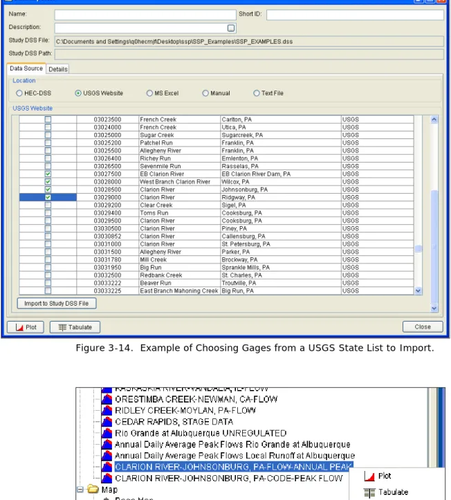
Once a state is selected, press the OK button and a list of the available gages from that state will appear in a pick list as shown in Figure 3-14. Check the boxes for all of the gages you would like to import and then press the Import to Study DSS File button. Once the import button is pressed, a process will begin during which the data will be
downloaded from the USGS website and saved to the study DSS file. HEC-SSP will automatically name the data when importing multiple gages at one time. The USGS import process will download annual peak flow data, and the USGS data quality codes. The quality codes will be added as an addition object to the Data folder.
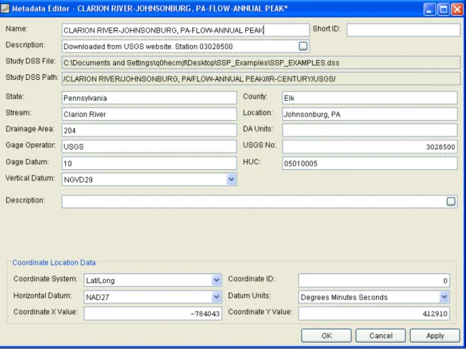
In addition to the data itself, any metadata that is available will be downloaded and stored with the data. The metadata can be viewed from the Details Tab on the Data Importer. Metadata can also be viewed or edited by opening the Metadata Editor. To open this
editor, place the mouse on top of a data object in the Data folder and click the right mouse button. The shortcut menu contains an Edit
Metadata option, as shown in Figure 3-15. The metadata editor is
shown in Figure 3-16.
Figure 3-16. Metadata can be Viewed or Edited by Opening the Metadata Editor.
As shown in Figure 3-16, the metadata consists of the State, County, Stream, Location, Drainage Area, DA Units, Gage Operator, USGS Gage No., Gage Datum, HUC (Hydrologic Unit Code), Vertical Datum, and a description field. Additionally, the coordinate location of the data is shown. The coordinate location consists of Coordinate System, Coordinate ID, Horizontal Datum, Datum Units, Coordinate X Value, and Coordinate Y Value. Most of the USGS data is retrieved with the Latitude/Longitude coordinate system as shown in the example. In addition to editing the metadata, the Metadata Editor allows the user to change the name of the data, enter a short identifier, and enter a longer description.
If the metadata does not download automatically, the user has the option to enter any of the information by hand. Metadata is not generated automatically for any of the other four data sources. Therefore, entering the metadata is required if the user wants it to be carried along with the study.
After the data is imported into the study, the user can select any one of the gages in the Data folder and Plot or Tabulate the data. The plot and tabulate options are available from the Data menu and from a shortcut menu that opens by clicking the right mouse button when the
pointer is located on top of the gage object in the Data folder. If you select the Plot option, you will get a plot of the peak flow data for that gage. If you select the Tabulate option, you will get a table
containing the data. Data values can be edited within the table; however, the editing mode must be turned on. To turn on editing, select the EditAllow Editing menu option. Use the FileSave or
FileSave As menu option to save the data when you are satisfied
with edits.
If the data has coordinate location information, it will then be plotted on top of the background maps. The software will convert the coordinates of the point data to the default coordinate system of the base map. The user can interact with the plotted points by right clicking on the gage icon in the map and a shortcut menu will appear as shown. The user has the option to edit the metadata, plot, tabulate, rename, or delete the data.
Performing the Bulletin 17B Flow Frequency Analysis
To perform a Bulletin 17B flow frequency analysis, go to the Analysis menu and select New Bulletin 17B Flow Frequency. This will
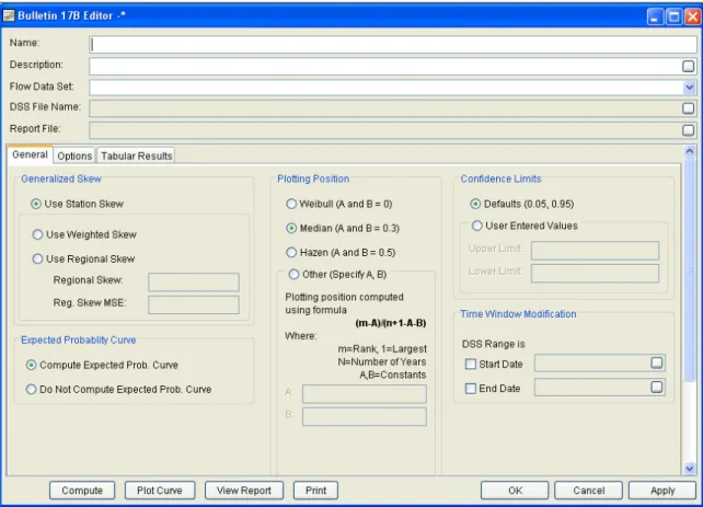
bring up an empty Bulletin 17B editor. As shown in Figure 3-17, the user must enter a name for the analysis, a description (optional), and select a flow data set (gage data stored in study DSS file). The DSS File Name and Report File are automatically filled in by the program. For now, the DSS File Name will be the study DSS file and the report file will have the same name as the analysis.
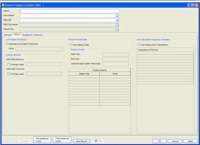
The editor window contains three tabs: General, Options, and Tabular Results. The General tab contains settings for Generalized Skew, Expected Probability Curve, Plotting Positions, Confidence limits, and a Time Window Modification. Default settings are already established for each of the options on the General tab; however, the user can change the default settings.
The Options tab contains information on Low Outlier Threshold, Historic Period Data, and User-Specified Frequency Ordinates. These options are not required for most analyses but may be necessary depending upon the data.
A detailed description of each of the Bulletin 17B settings and options can be found in Chapter 5, Performing a Bulletin 17B Flow Frequency Analysis. Once all of the settings and options have been selected, the user presses the Compute button to have the computations
performed. When the computations have finished a message window will open stating Compute Complete. Press the OK button on the
message window to close the window. Once the computations have finished the user can begin to look at output.
Figure 3-17. Bulletin 17B Flow Frequency Analysis Editor.
Viewing and Printing Results
Tabular output can be viewed by selecting the Tabular Results tab. When this tab is pressed, a set of tables will appear as shown in Figure 3-18. The primary table on the Tabular Results tab consists of percent chance exceedance, computed flow frequency curve, the expected probability adjusted curve, and the 5 and 95 percent confidence limits. The second table (bottom left) contains general statistics about the data, such as the mean, standard deviation, station skew, regional skew, weighted skew, and the adopted skew of the analysis. The third table (bottom right) contains the number of historic events, high outliers, low outliers, zero or missing values, systematic events in the data set, and the number of years in the historic period. The table can be sent to the printer by pressing the
Print button at the bottom of the analysis window. The user can
control the number of decimal digits shown in the result tables and in reports. Select Options from the Tools menu and then open the
Figure 3-18. Tabular Results of Bulletin 17B Editor.
Graphical output can be obtained by pressing the Plot Curve button at the bottom of the analysis editor. When this button is pressed, a plot will appear like the one in Figure 3-19. This plot contains the
computed frequency curve, the expected probability adjusted curve, the confidence limits, and the data points plotted by the user-selected plotting position method. Additionally, a plot title is listed at the top. The plot title is by default the user-defined name of the analysis. The user can modify the plot properties by selecting the EditPlot
Properties menu option. A plot properties window will open that lets
the user change the line style for each data type, change the axis labels, modify the plot title, and edit other plot properties. The user can also edit line styles by placing the mouse on top of the line or data point in the plot or legend and clicking the right mouse button. Then select the Edit Properties menu option in the shortcut menu. The plot can be printed or sent to the windows clipboard by using the Print and Copy to Clipboard options found under the File menu.
Point to add a point. Draw properties can be edited for these
user-defined lines and points by placing the mouse on top of the point or line and clicking the right mouse button. Then select the Edit
Properties option in the shortcut menu.
Figure 3-19. Flow Frequency Curve Plot.
The final piece of output available from a flow frequency analysis is a text report file. The report file lists all of the input data and user settings, plotting positions of the data points, intermediate results, each of the various statistical tests performed (i.e. high and low outliers, historical data, etc.), and the final results. This file is often useful for understanding how the software arrived at the final
frequency curve. Press the View Report button at the bottom of the analysis editor to view the report file. When this button is pressed, a window will appear containing the report as shown in Figure 3-20.
C H A P T E R 4
Using the HEC-SSP Data Importer
The HEC-SSP Data Importer is used to import, enter, and view data and the corresponding metadata used in an HEC-SSP study. The current version of HEC-SSP can be used to import annual peak data (flow and stage) and data stored at regular intervals, like hourly flow data.
Contents
• Developing a New Data Set
• Importing Data from an HEC-DSS File
• Importing Data from the USGS Website
• Importing Data from an Excel Spreadsheet
• Entering Data Manually
• Entering Data from a Text File
• Metadata
Developing a New Data Set
Before any analyses can be performed in HEC-SSP, the user must import or enter data into the study. Importing, entering, and viewing data is accomplished in the Data Importer. To open the data
importer, go to the Data menu and select New from the list of options. This will bring up a data importer as shown in Figure 4-1.
Figure 4-1. HEC-SSP Data Importer.
At the top of the Data Importer, the user can enter a Name for the new data set. Optionally, the user can enter a short identifier (limited to 16 characters) and a Description of the data set. The study DSS file name is provided. The DSS file is used for storing the data for the study. The user does not have to enter a name when importing or manually entering data. The program will automatically name the data using USGS names or HEC-DSS pathname parts. If a Name is
entered then it will be combined with the USGS gage name or HEC-DSS pathname parts to create a unique name. The user can rename a data set by selecting the data set in the study explorer and clicking the right mouse button. A shortcut menu should open with a Rename menu option. The Data menu also contains a Rename menu option;
however, the data set must be selected in the study explorer before this menu option is active.
The Data Importer contains two main tabs, Data Source and Details. The Data Source tab is used for importing or entering data manually while the Details tab is used to describe the data (i.e. metadata). The
Data Source tab contains five options for getting data into the study
DSS file: Importing from an existing HEC-DSS file, importing from the USGS Website, importing from an Excel spreadsheet, entering the data manually, and importing from a text file.
Importing Data from an HEC-DSS File
To import data from an HEC-DSS file into the HEC-SSP study DSS file, first select the HEC-DSS radio button on the data importer. Selecting
HEC-DSS will change the view of the Data Importer to look like Figure
4-2.
Figure 4-2. Data Importer with HEC-DSS Import Option.
pathnames will be filled with the records that are contained in that DSS file. The user can reduce the number of listed pathnames by selecting pathname parts to filter in the pathname part selection area just above the table. Any pathname part can be used to filter the list down to a more manageable number of pathnames to select from. The user can then select pathnames to import by double clicking on one or more of the listed pathnames in the table. Each selected pathname will show up in the list below the table. Once the user has selected all of the pathnames that they want to import, pressing the
Import to Study DSS File button enacts the import process. An
HEC-SSP data set will be developed for each pathname that was selected.
Importing Data from the USGS Website
The second way to import data into HEC-SSP is to use the USGS
Website option. When this option is selected, the data importer will
look like Figure 4-3.
The first step in using the USGS import option is to select a data type to import (e.g. Annual Peak Data). Then choose to import Flow and/or Stage data. Next the user should select the Get USGS
Station ID’s by State button. Selecting this button will bring up a
small window that allows the user to select a state in which to acquire data, as shown in Figure 4-4.
Figure 4-4. Window to Select a State for Importing USGS Data.
Once the user selects a state and presses the OK button, a process will begin in which all of the gage locations for that state will be downloaded from the USGS website. A listing of all the gages for that state will then be displayed in the table at the bottom of the data importer. An example of the data importer with a list of USGS gages is shown in Figure 4-5.
Figure 4-5. Data Importer with USGS Gages Listed in Table.
The next step is to select the desired gages for importing into the HEC-SSP study. The user can filter the list to a smaller number of gages by using the filter drop down boxes at the top of the table. To select a gage for importing, simply check the box in the left hand column for each gage location that is to be imported. After all of the desired locations are selected, press the Import to DSS File button to import the data into the study DSS file. Pressing this button will start a process of downloading data from the USGS website. For each
selected location, the software will download the Data Quality Codes if they are available. The program issues a message that data quality codes are available and adds the codes as an additional data set to the Data folder. For an explanation of the codes, please visit the USGS website.
Warning: all data downloaded from the USGS website should be
reviewed to ensure it is appropriate before any analyses are performed on the data. Some data stored on the USGS website are estimated, not measured. The user should check the data on the USGS website and be aware of the quality of all the data before using it. HEC-SSP will import the annual peak flow and stage quality codes (the program does not import quality codes for daily, instantaneous, and real time
data). A description of the quality codes for annual peak flows is contained in Table 4-1 and a description of the quality codes for annual peak stages is contained in Table 4-2.
Table 4-1. Quality Codes for USGS Annual Peak Flow Data.
Code Description
1 Discharge is a Maximum Daily Average
2 Discharge is an Estimate
3 Discharge affected by Dam Failure
4 Discharge less than indicated value which is Minimum Recordable Discharge at this site 5 Discharge affected to unknown degree by Regulation or Diversion
6 Discharge affected by Regulation or Diversion
7 Discharge is an Historic Peak
8 Discharge actually greater than indicated value
9 Discharge due to Snowmelt, Hurricane, Ice-Jam or Debris Dam breakup
A Year of occurrence is unknown or not exact
B Month or Day of occurrence is unknown or not exact
C All or part of the record affected by Urbanization, Mining, Agricultural changes, Channelization, or other
D Base Discharge changed during this year
E Only Annual Maximum Peak available for this year
Table 4-2. Quality Codes for USGS Annual Peak Stage Data.
Code Description
1 Gage height affected by backwater
2 Gage height not the maximum for the year
3 Gage height at different site and(or) datum
4 Gage height below minimum recordable elevation
5 Gage height is an estimate
6 Gage datum changed during this year
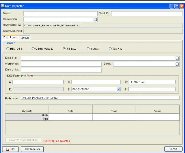
Importing Data from an Excel Spreadsheet
The third option for importing data into HEC-SSP is MS Excel. When this option is selected, the data importer will change as shown in Figure 4-6. The first step in importing data from an Excel spreadsheet is to select browse button, , at the end of the Excel File field. Once an Excel file is selected, a data view window will open showing the data contained in the selected spreadsheet. An example Excel® Data
Figure 4-7. Example Excel Data Viewer.
The next step is to highlight the date and data values to be imported into the study (only highlight the data, not the column headings). The data must be in a format of Date in the first column and Data in the second column. The date must be in the Day, Month, Year format (ddmmyyyy) as shown in Figure 4-7. Next, press the OK button and the data will be placed in the table at the bottom of the editor. The last step before importing the data is to specify the units of the data, and each of the pathname parts for storing the data in the study DSS file (make sure to edit the C-part pathname if data is not annual peaks). Enter units of cfs for data in cubic feet per second or units of
cms for data in cubic meters per second. The final step is to press the Import to Study DSS File button, and the data will be imported.
Entering Data Manually
Another option for getting data into the study is to enter the data manually. When the Manual option is selected, the window will change to what is shown in Figure 4-8.
Figure 4-8. Data Importer with Manual Data Entry Option Selected.
To enter data manually, the user enters a name for the data set at the top, along with a short identifier and a description (optional). A
starting date and time must be entered. The units of the data must also be defined as well as the data type. The last step before entering the data is to specify the pathname parts for how the data will be stored into the study DSS file. This requires the user to enter a label for the A, B, C, E, and F part of the DSS pathname. Once all of the data labeling is completed, the data can be entered into the table at the bottom of the editor. The user must enter the Date, Time, and data Value for each peak flow value to be entered. After a Date, Time, and Value are entered into a row, a new row will be generated in the table when the user leaves the Value field. The date must be in the Day, Month, Year format (ddmmyyyy). Another option for getting data into the table is to copy it to the clipboard and then paste it into
the table. The table supports pasting data one column at a time or you can paste the date, time, and value information all at once. When all of the data are entered into the table, the user presses the Import
to Study DSS File button and the data will be stored in the study DSS
file.
Importing Data from a Text File
The fifth option for importing data into HEC-SSP is a comma delimited
Text File. When this option is selected, the data importer will change
as shown in Figure 4-9.
Figure 4-9. Data Importer with Text File Option Selected.
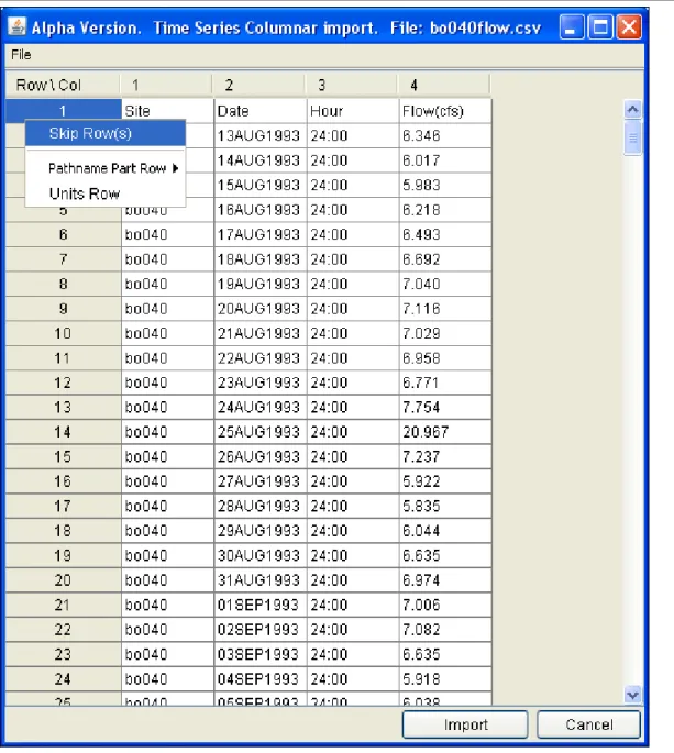
The first step in importing data from a comma delimited Text File is to press the Select File, , button at the end of the File field. Once a comma delimited text file is selected, a data view window will open showing the data contained in the selected file. An example text file data viewer is shown in Figure 4-10.
Figure 4-10. Example Text File Data Viewer.
The next step is to highlight the date, time, and data columns. Only highlight the data that will be imported, not the column headings. If there are column headings then they need to be identified. To do this, select the row or rows that do not contain data to be imported. Then click the right mouse button and select the Skip Row(s) menu option, as shown in Figure 4-11.
Figure 4-11. Identify Rows that do not Contain Data to be Imported.
To identify the date and time columns, place the mouse pointer on the column number at the top of the table and click the right mouse button. Then move the mouse pointer to the Date – Time Column option to see an additional menu of options, as shown in Figure 4-12. Figure 4-12 shows that column 2 will be defined as the date column. The date must be in the Day, Month, Year format (ddmmyyyy). The data viewer will highlight the date and time columns once they have been defined.
Figure 4-12. Identify Date and Time Columns.
To define the data column, place the mouse pointer on the column number at the top of the table and click the right mouse button. Then choose the Set Data Column menu option from the shortcut menu. Another editor will open, as shown in Figure 4-13, that allows the user to define the pathname parts, data units, and data type. After
defining these data properties, click the Import Now button to import the data and data properties into the Data Importer. You can edit the data values or data properties in the data importer before importing the data to the study. The final step is to press the Import to Study
Figure 4-13. Editor for Defining the Data Properties.
Metadata
When downloading data from the USGS website, in addition to the raw data, the software will also attempt to download any metadata
available for each gage location. When using one of the other four methods for importing data, the user can manually enter metadata by selecting the Details tab, as shown in Figure 4-14. The metadata consists of the State, County, Stream, Location, Drainage Area, DA Units, Gage Operator, USGS Gage No., Gage Datum, HUC (Hydrologic Unit Code), Vertical Datum, and a description field. Additionally, the coordinate location of the data is shown. The coordinate location consists of Coordinate System, Coordinate ID, Horizontal Datum, Datum Units, Coordinate X Value, and Coordinate Y Value. If coordinate system data are entered, data icons and text labels will show up on the background map at the specified locations.
Metadata can be viewed and edited any time after the data has been imported into the study by opening the Metadata Editor. To open the Metadata Editor, place the mouse pointer on top of a data set in the Data folder and then click the right mouse button. Choose the
Edit Metadata option from the shortcut menu, as shown in Figure
4-15. The Metadata Editor will look exactly like the Details tab on the Data Importer. The Metadata Editor can also be opened from the Data menu and from a shortcut menu that opens by right clicking on a data icon in a background map.
Figure 4-14. Details Tab on the HEC-SSP Data Importer.
Plotting and Tabulating the Data
After the data is imported into the study, the user can select any one of the data sets in the study explorer. A shortcut menu will open when clicking the right mouse button while a data set is selected. The
shortcut menu contains options to change the name, plot, and tabulate the data. These options are also available from the Data menu;
however, the data must be selected in the study explorer before these options are available. If you select the Plot option, you will get a plot similar to the one shown in Figure 4-16.
Figure 4-16. Plot of Peak Annual Flow Data.
If you select the Tabulate option, a table will open with the data listed as shown in Figure 4-17. Data values in the table can be edited after selecting the EditAllow Editing menu option. To save any edits,
C H A P T E R 5
Performing a Bulletin 17B Flow
Frequency Analysis
The current version of HEC-SSP allows the user to perform flow
frequency analyses based on Bulletin 17B, "Guidelines for Determining Flood Flow Frequency" (March 1982). This chapter discusses in detail how to perform a Bulletin 17B Flow Frequency Analysis in HEC-SSP.
Contents
• Starting a New Analysis
• General Settings, Options, and Computations
Starting a New Analysis
A flow frequency analysis can be started in two ways within the
software, either by right clicking on the Bulletin 17B folder in the study explorer and selecting New, or by going to the Analysis menu and selecting New and then Bulletin 17B Flow Frequency. When a new flow frequency analysis is selected, the Bulletin 17B Editor will appear as shown in Figure 5-1.
Figure 5-1. Bulletin 17B Flow Frequency Analysis Editor.
The user is required to enter a Name for the analysis, while a
Description is optional. An annual peak flow data set must be
selected from the available data sets stored in the current study DSS file (see chapter 4 for importing data into the study). The list of data that can be selected for a Bulletin 17B analysis will only include those data that have an irregular interval, like IR-CENTURY and IR-YEAR (E-part pathname). Once a Name is entered, and a flow data set is selected, the DSS File Name and Report File will automatically be populated. The DSS filename is by default the study DSS file. The report file is given the same name as the analysis with the extension ".rpt".
General Settings, Options, and Computations
Once the analysis name and flow data set are selected, the user can begin setting up the analysis. Three tabs are contained on the Bulletin 17B editor. The tabs are labeled General, Options, and Tabular
Results.
General Settings
The first tab contains general settings for performing the flow frequency analysis (Figure 5-1). These settings include:
• Generalized Skew
• Expected Probability Curve
• Plotting Positions
• Confidence Limits
• Time Window Modification
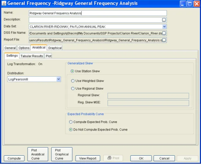
Generalized Skew
There are three options contained within the generalized skew setting: Use Station Skew, Use Weighted Skew, and Use Regional Skew. The
default skew setting is
Use Station Skew.
With this setting, the skew of the computed curve will be based solely on computing a skew from the data points contained in the data set. No weighting will be performed to compute the final skew.
The Use Weighted Skew option requires the user to enter a generalized regional skew and a Mean-Square Error (MSE) of the generalized regional skew. This option weights the computed station skew with the generalized regional skew. The equation for performing this weighting can be found in Bulletin 17B (equation 6). If a regional skew is taken from Plate I of Bulletin 17B (the skew map of the United States), the value of MSE = 0.302.
The last generalized skew option is Use Regional Skew. When this option is selected, the user must enter a generalized regional skew and an MSE for that skew. The program will ignore the computed station skew and use only the generalized regional skew.