TI 2007-034/2
Tinbergen Institute Discussion Paper
Interlocking Boards and Firm
Performance:
Evidence from a New Panel Database
Mariëlle Non
1Philip Hans Franses
1,21 Erasmus Universiteit Rotterdam, and Tinbergen Institute; 2 Econometric Institute.
Tinbergen Institute
The Tinbergen Institute is the institute for economic research of the Erasmus Universiteit Rotterdam, Universiteit van Amsterdam, and Vrije Universiteit Amsterdam.
Tinbergen Institute Amsterdam Roetersstraat 31
1018 WB Amsterdam The Netherlands
Tel.: +31(0)20 551 3500 Fax: +31(0)20 551 3555 Tinbergen Institute Rotterdam Burg. Oudlaan 50
3062 PA Rotterdam The Netherlands
Tel.: +31(0)10 408 8900 Fax: +31(0)10 408 9031
Most TI discussion papers can be downloaded at http://www.tinbergen.nl.
Interlocking Boards and Firm Performance:
Evidence from a New Panel Database
Mari¨elle C. Non
∗Philip Hans Franses
†March 29, 2007
Abstract
An interlock between two firms occurs if the firms share one or more di-rectors in their boards of didi-rectors. We explore the effect of interlocks on firm performance for 101 large Dutch firms using a large and new panel database. We use five different performance measures, and for each performance mea-sure we design three different panel data models, where we allow the effect of the number of interlocks to be linear, quadratic or square root, either with or without lags.
Based on all results we conclude that current interlocks can have a negative effect on future firm performance. We show that this negative effect is jointly established by (1) interlocking directors being too busy and (2) by directors being members of a homogenous upper class group.
Keywords: interlocks, firm performance JEL codes: C23, G34, J53, Z13
∗Corresponding author: Tinbergen Institute and Department of Economics, Erasmus
Univer-sity Rotterdam, P.O. Box 1738, 3000 DR Rotterdam, The Netherlands. E-mail: [email protected]. Earlier versions of this paper have been presented at various seminars. We thank the participants for their helpful comments and suggestions. We thank Lotje Kruithof for her help with compiling the database.
†Econometric Institute and Department of Business Economics, Erasmus University Rotterdam,
1
Introduction
A director can hold several directorships in different firms. Such a director consti-tutes a link between the firms. Firms that are linked in this way are interlocked. There is much research on interlocks, ranging from a description of what the net-work of interlocked firms looks like to studies on the influence of interlocks on firm strategy and performance. We address this last topic by analyzing a new large and unique panel data set concerning firms in The Netherlands.
There are several views on the origin and effect of interlocks, see Mizruchi (1996) for an extensive review. Here we mention four well-known views. The first is that interlocks are a way for firms to coopt and/or monitor each other (Dooley, 1969 and Mizruchi and Stearns, 1994). The second view states that interlocks provide firms with information on business practice (Davis, 1991). The third is that interlocks merely reflect upper-class cohesion (Useem, 1984). And, fourth, the recently put forward busyness hypothesis of Ferris et al. (2003) states that multiple directorships place an excessive burden on directors (see also Fich and Shivdasani, 2006). The first two views predict a positive influence of interlocks on firm performance. In contrast, the busyness hypothesis predicts anegativeinfluence on firm performance. Finally, the effect of interlocks can be either positive, negative or neutral when interlocks reflect upper-class cohesion. So, only the upper class cohesion theory and the busyness hypothesis can explain a negative effect of interlocks on performance, the other two views predict a positive effect1
.
When interlocks would indeed reflect upper class cohesion the effect of interlocks can be either positive, negative or neutral. The argument that interlocks in this case have a negative effect proceeds as follows. In The Netherlands there is a cohesive upper class of directors, who often have more than two directorships and meet each other regularly (see Stokman et al., 1988, and Van Hezewijk, 1986, 1988). The boards of firms with many interlocks per director apparently consist of directors who mostly belong to this particular cohesive upper class. Cohesive groups perform worse in decision making, as they strive for unanimity and often suffer from a reduction in independent critical thinking (see Janis, 1982, and Mullen et al., 1994). Moreover,
the members of the Dutch cohesive upper class mostly have the same background (Van Hezewijk, 1986, 1988) and hence such a board is less diverse, while it is precisely such diversity that has been shown to improve firm performance (see Carter et al., 2003).
Given the different views, it is not surprising that much empirical research on the effect of interlocks on performance has been carried out. Results of these studies are mixed, see for example Bunting (1976), Pennings (1980), Burt (1983), Fligstein and Brantley (1992), and Phan et al. (2003). Note that most research is based on US data. We are aware of only two studies which concern The Netherlands, and these are Meeusen and Cuyvers (1985) and Van Ees et al. (2003). The first study documents a positive relation between interlocks within financial firms and their performance. The second study mentions a negative effect of the percentage share of outsiders on firm performance, where outsiders are defined as directors who have at least two directorships.
In our present paper we again take up the issue of interlocks and performance by presenting empirical results based on a newly created large panel database for The Netherlands. In contrast to previous studies, our database constitutes a panel for many years, instead of the commonly used cross section. Hence, we can also examine the dynamic effects of interlocks, which, as we will document, are quite prominent. In the first part of our paper we explore the relation between the number of interlocks and firm performance. If we find an effect for some models and some com-binations of variables it is a negative effect. This effect matches with the busyness hypothesis and with the cohesive group theory. In the remainder of the paper we seek to establish which of the two is most plausible, at least for the data at hand. Looking at the results of various regressions leads us to conclude that we cannot clearly distinguish between the two hypotheses, as both seem partly valid.
The outline of the paper is as follows. First, in Section 2 we give a description of our data. Next, in Section 3, we will set out the method we use to investigate the effect of the number of interlocks on firm performance. The results of applying this method to the data are presented in Section 4. In Section 5 we elaborate on possible explanations of the negative influence of interlocks on performance and in Section 6
we summarize our findings.
2
A new panel database
In The Netherlands virtually all firms have a two-tier board structure. There is an executive board, which consists of a Chief Executive Officer (CEO), a Chief Fi-nancial officer (CFO) and of other executive directors. Additional to this executive board, there also is a supervisory board. The main task of this board is to monitor the executive board itself and to monitor the major business decisions taken by the executive board. The supervisory board largely consists of retired executive direc-tors. Almost all of the interlocks of a firm are formed by members of the supervisory board who also serve as supervisory director for other firms. It is not uncommon for a high-profile director to have four or five supervisory directorships. As interlocks are mainly formed by the supervisory board, we focus on these directors.
Defining interlocks
We gathered data on supervisory boards of 101 large, listed, Dutch firms in the period 1994 to 2004, using annual reports and the REACH database. The annual reports give us, for each firm, the directors in the supervisory board by the end of July in each year. Using this information, we count the number of interlocks of a firm with other firms in the database. For example, suppose firm A has two directors, X and Y. X also sits on the supervisory boards of firms B and C, and Y also sits on the board of firm D. As such, firm A then has three interlocks. Multiple interlocks are counted as one. Suppose Y is on the boards of A, D and also B, like X. Then, firm A still has only three interlocks, as the multiple interlock with firm B is counted as one interlock.
We divide the number of interlocks by the number of directors to correct for the size of the board2
. In our database there are a few firms with very large boards (15 or more members) as well as firms with smaller (3 or less members) boards. Clearly, large boards can have much more interlocks than small boards.
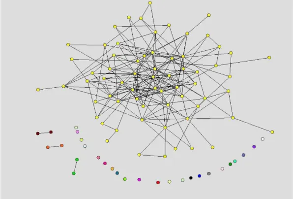
to measure the directors’ experience and busyness, while the number of interlocks itself is the best variable to measure the amount of information the firm gets about its environment. We therefore did the same analysis as reported below using the number of interlocks instead of the number of interlocks divided by the size of the board, and the results are qualitatively the same. In what follows we will therefore use the term ’interlocks’ for the number of interlocks divided by the size of the board. Figure 1 shows the network of interlocks for the year 1998. For other years the network looks roughly the same (although of course various little changes occur over time). We see one giant component of firms that are linked to each other and several fringe firms that have no links or are only linked to another fringe firm.
Performance measures
Additional to information on the supervisory boards, we also gathered data on the performance of the firms during 1994 to 2004 using the REACH database. We gathered data on stock returns, the price-earnings ratio and the price-to-book ratio, the return on assets and the return on equity. Furthermore, for each firm we store the BIK codes3
(four-digit level), the turnover and the growth of the turnover. Some of the dependent variables (stock returns, the price-earnings ratio and the price-to-book ratio) show serious skewness and excess kurtosis. To accommodate this, we transform the stock return by taking the log of (1 + return/100). For the price-earnings ratio we delete all observations on firms that make losses, as the price-earnings ratio is not defined for these firms. We then transform the resulting price-earnings ratios by taking natural logs. Finally, the price-to-book ratio is also taken in natural logs.
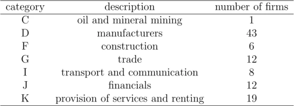
We have the BIK codes of the firms in the sample at the four-digit level. Most firms have several BIK codes as our database concerns large firms active in several related areas. For each firm we take the main sector in which it is active and reduce the corresponding BIK code to the one-digit level. This way, firms are divided in seven different groups, like finance, transport and communication, industry, and construction. In Table 1 these categories are summarized.
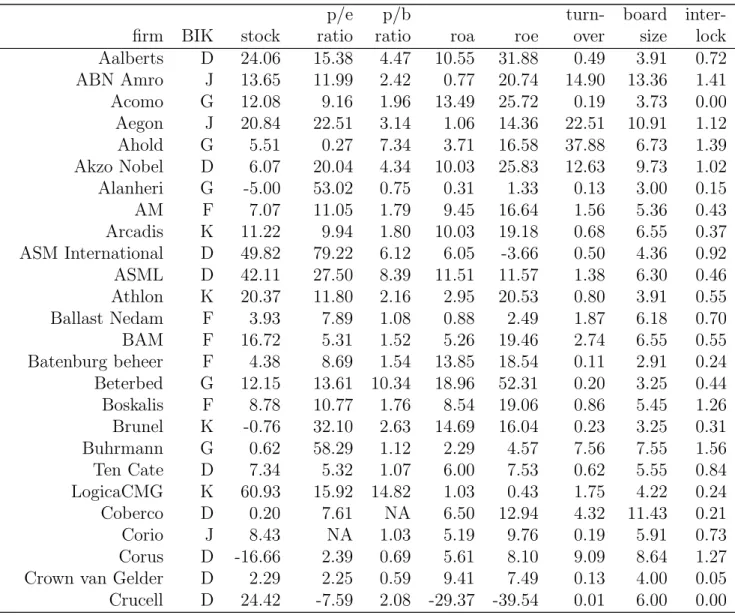
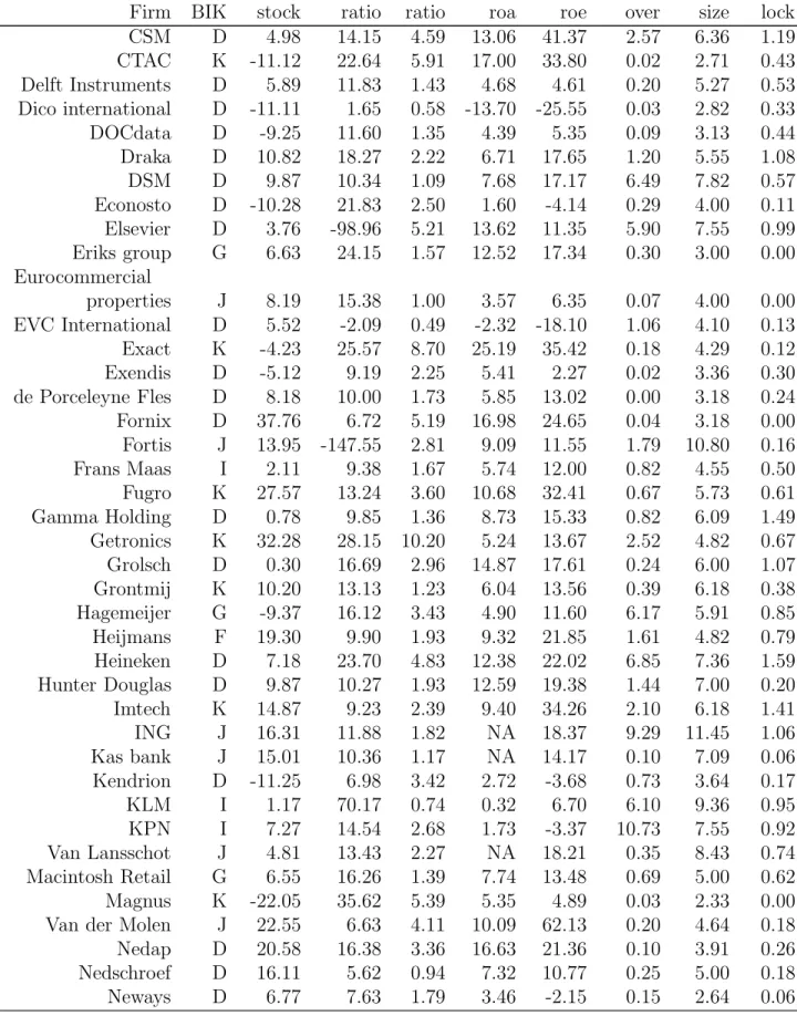
We report the BIK code of the firm and the average values (over the years) of the untransformed performance measures, the turnover, the board size and the number of interlocks per director. From this table it is clear that the firms differ widely on these features.
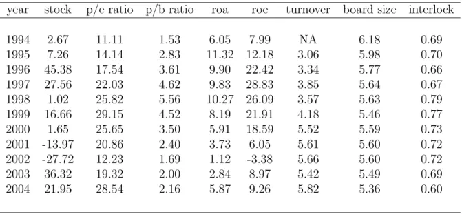
In Table 3 we give statistics per year, now averaged over all 101 firms. We report the averages of the untransformed performance measures, the turnover, the board size and the number of interlocks per director. For the number of interlocks per director we exclude all firms that started only after 1994. These firms have somewhat lesser interlocks per director and, consequently, when these firms are included the number of interlocks per director decreases over time. As one can see from the last column of Table 3, the number of interlocks per director does not have a clear upward or downward trend. Interestingly, the size of the board declines over time, also when the firms that start after 1994 are excluded. As expected, we see that the average firm performance is lower during 2001 and 2002 and we also note that the turnover increases over time.
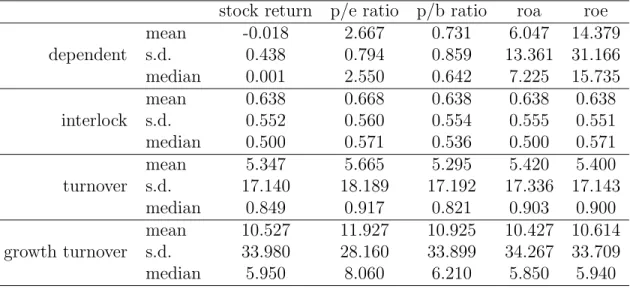
For Tables 2 and 3 we used all available observations for the computations. However, for the regressions below we need to delete all firm-year observations that have either a missing value on one of the performance measures or on turnover or growth of turnover. We also removed some outliers. In Table 4 we report the available sample sizes for the five performance measures. The sample size clearly differs between performance measures. In Table 5 we give some statistics of the (transformed) data, using the samples of Table 4. From Table 5 one can see that the statistics differ only slightly between the different performance measures.
3
Methodology
We have five different financial performance measures and we analyze each of these separately. For each performance measure we estimate the parameters of three different regression models. The (panel data) models we use are a fixed effects (FE) model, a random effects (RE) model and a model based on the BIK codes. We will denote this last model as the BIK model. We use the AIC for model selection as,
in contrast to the BIC, this criterion yields plausible final models. This AIC-based selected model is used to draw conclusions.
Models
The FE model is given by
yit=αi+xitβ+γt+εit, (1)
with εit iid and normally distributed, yit the dependent variable, where xit collects
the independent variables and γt measures developments over time 4
. Note that the constant αi depends on the firm i. The estimator ofβ is the within-estimator, as it
is based on differences over time within a firm, and not on differences between firms. The RE model is written as
yit =α+xitβ+γt+αi+εit, (2)
with both εit and αi iid and normally distributed. Again, yit is the dependent
variable,xit summarizes the independent variables and γt concerns time. Note that
here α does not depend on the firm i. Instead, correlation in the data of the same firm over time is captured by a random variableαi, which is the same over time for
one firm, but potentially differs across firms. The error termζit =αi+εit is not iid
and normally distributed asζit and ζi,t−1 are correlated. The resulting estimator of β is based on differences within a firm over time as well as on differences between firms.
For the BIK model, let BIKi denote the BIK code of firm i. The BIK model is
given by
yit=αBIKit+xitβ+εit, (3)
with εit iid and normally distributed. The idea of including αBIKit is that firms in
the same sector might have the same performance over time. For example, over time the patterns in stock returns might be the same for firms in the same sector. Note that with the BIK model we allow for different patterns over time. For instance, the model allows the performance in sector 1 to increase while at the same time
the performance in sector 2 decreases. Note that this is not possible with the time dummies in the FE and RE models.
Variables
As independent variables in the three models we use the variable ’interlock’, defined in the previous section, as well as some control variables. These control variables are the same for each of the performance measures. We include turnover, squared turnover, turnover one year lagged, squared turnover one year lagged, growth of turnover (in short: growth), squared growth, growth one year lagged and squared growth one year lagged. With the squared variables we allow for a potential nonlinear effect of the control variables on performance. Note that turnover serves as a measure of the size of the firm.
We estimate the parameters in each of the three models three times. First, we include ’interlock’ linearly, next we include ’interlock’ quadratically and finally we include the square root of ’interlock’. We do this as previous research in for example Bunting (1976) indicates that the effect of ’interlock’ could be nonlinear. As a theoretical explanation for a nonlinear effect one could think of a combination of the ’information on business practices’ theory and the busyness hypothesis. In this case, having more interlocks would lead to more information but also to more busy directors. When the number of interlocks is low, directors are not yet time-constrained and therefore more interlocks would lead to a better performance. On the other hand, when the number of interlocks is already high, adding more interlocks would not lead to much more information while the directors, who are already busy, would get even more time-constrained, leading to worse performance. Hence, the nonlinear relation would then be an inverted U-shape.
As we have a panel database it is also possible to estimate the models while including ’interlock’ with a one year lag. This allows us to see if there is a time lag in the effect, that is, whether the effect of interlocks is immediately visible or whether it takes some time before the effect can be noticed. Another advantage of using ’interlock’ one year lagged is that it enhances the robustness of the estimates. Indeed, some researchers have expressed concern on the possible reverse causality
between the number of interlocks and firm performance. Not only will the number of interlocks influence performance, but good performing firms could attract more interlocking directors. In the database we use, the number of interlocks is based on the directorships halfway the year, while performance is measured over the complete year, and is quite volatile over years. Hence, perverse causality is unlikely to happen and by including lagged interlocks we can even exclude this situation.
4
The main empirical results
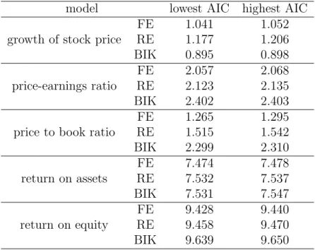
We only report the results on the models (FE, RE or BIK) that have the lowest AIC, which means that for the stock returns we only report the results of the BIK model, while for the other performance measures the FE model has the lowest AIC. Table 6 summarizes the AIC values of the models. It is not surprising that the BIK model is favored for stock returns. In the sample there is both a boom (before 2000) and a decline (after 2000) of stock prices. It is well known that stock prices in some sectors lead booms and declines, while others sectors follow. Allowing for different patterns over time for different sectors seems to be reasonable here, and hence the favorable AIC values for the BIK model.
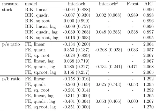
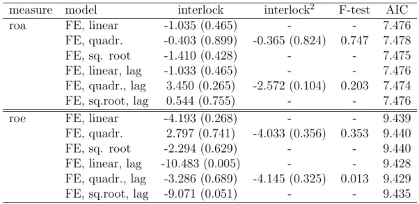
In Tables 7 and 8 we report the estimation results of the method outlined in the previous section. Each panel of the tables has a different performance measure as the dependent variable in the panel model. We report parameter estimates on ’interlock’, as well as the relevant p-values, the AIC and for the quadratic models the p-value of an F-test testing the joint significance of the linear and quadratic term. We estimate the FE, RE and BIK model, using a linear, quadratic and square root specification of ’interlock’. Moreover, we estimate the same models using ’interlock’ one year lagged. In each model we also include the control variables mentioned in the previous section (estimation results are not reported to save space).
When looking at the results, we note that the effect of the number of interlocks on stock returns (Table 7), the price-earnings ratio (Table 7) and the return on assets (Table 8) is not significant. On the other hand, the effect on the price-to-book ratio (Table 7) and the return on equity (Table 8) is (partly) significant5
the price-to-book ratio, all parameters for current interlocks are significant at the 5% or 10% level and the parameters for lagged interlocks are significant at the 1% level. For return on equity only the lagged variables are relevant. The significant estimates in the linear and square root specifications are all negative. The estimated quadratic specification has a U-shape with minimum at approximately 3.9 interlocks per director for the pricetobook ratio and an inverted Ushape with maximum at -0.4 interlocks per director for return on equity (lagged specification). As the number of interlocks per director is a positive variable with a mean of approximately 0.65 and a standard deviation around 0.55, the significant quadratic specifications also suggest a negative effect.
In the models above both lagged and current interlocks are used as independent variables. The AIC values in the last columns of Tables 7 and 8 allow us to compare the performance of the contemporaneous specification with the performance of the lagged specification. For the price-to-book ratio and the return on equity the lagged specification gives a better AIC, while for stock returns, the price-earnings ratio and the return on assets the evidence is mixed. We note that the first two performance measures give clear-cut results, especially in the lagged specification.
All this leads us to conclude thatifthere is an effect of interlocks on performance, this effect is negative and it occurs with a lag.
5
What could explain our findings?
Now we have found a small negative effect of the number of interlocks per director on firm performance, we wonder which of the two theories could dominate in predicting a negative influence of interlocks. In this section we take a closer look at these theories.
The busyness hypothesis
First there is the busyness hypothesis of Ferris et al. (2003). Directors who gather many directorships get short of time and the performance of their firms deteriorates. This has already been noticed by Mace (1971) for the US case. Recent evidence
for the US is documented by Fich and Shivdasani (2006). In The Netherlands the situation is somewhat different, as the supervisory directors almost all are retired, and a supervisory directorship is not a full-time job. It is however widely acknowl-edged that having three or four directorships should be the maximum. The recently introduced Dutch corporate governance code (the so-called code Tabaksblat) advises that no director in the board should have more than five directorships, with a chair position counting twice. To investigate whether having busy directors on the board has an influence on performance we construct a variable that measures the ’busyness’ of the board and include this variable in the models.
For each director in our database we count his or her number of directorships. In line with the code Tabaksblat, we define a director as being busy when he has more than four directorships. The reason not to use five as a threshold is that the number of directors with more than five directorships is very limited. In addition, we have no information on chair positions and therefore cannot count these positions twice. For each firm and year we then count the number of supervisory directors in the board, and the number of these directors who are not busy (at least, according to our definition). Division of these numbers gives the fraction of non-busy directors in the board. We include this variable in a linear fashion. If the busyness hypothesis would hold true, the effect of the fraction of non-busy directors on firm performance should be positive. Before we examine this hypothesis empirically, we first address the second possible cause of our findings.
Homogeneous upper class
The second hypothesis of why interlocks have a negative effect on performance has to do with (the absence of) diversity in the board and a homogenous upper class of directors. In The Netherlands there seems to be an upper class of directors, who meet each other regularly, either in the boardroom or in all kinds of elite clubs. This has for instance been documented by Van Hezewijk (1986, 1988). The members of this upper class of directors have several directorships, mostly have the same background and as they meet regularly they often exchange opinions. They therefore can be called members of a homogenous group. It has been shown that diversity in
the board enhances the performance of the firm. We propose that for a firm it is therefore best to have a mixed board, with some directors belonging to the upper class and some not. If this is indeed true, heavily interlocked firms have mostly upper class directors and so would perform worse than other firms.
To test this upper class hypothesis we define a director as belonging to the upper class when he has three or more directorships. We then calculate for each firm and year the fraction of non-upper class directors in the board. We will include this variable in the model in a quadratic way, to allow for the optimal fraction to be somewhere between 0 and 1, which indicates a positive effect of diversity.
Limitations
We acknowledge that both measures above could have errors. First, a busy director is defined as having more than four directorships in our dataset. We capture 101 large firms in The Netherlands, but there are of course other firms either in The Netherlands or abroad that a director could serve, and we do not count these direc-torships. Furthermore, some directors are also active in government organizations, like the Dutch central bank. This information is however not available, and so we can only use the 101 firms in our dataset. We however believe that this is a reason-able proxy as for busyness we capture almost all Dutch listed firms, and only very recently there have been some signs of internationalization in the Dutch boardrooms in the sense that Dutch directors get a position in foreign firms and foreign directors get a supervisory directorship in Dutch firms.
According to our upper class measure, a director belongs to the upper class if he or she has more than two directorships. As with the busyness measure we only look at directorships in our 101 firms in the dataset. Also, the threshold of having more than two directorships is not based on previous evidence. Therefore, we also estimated the model using a threshold of more than one directorship and using a threshold of more than three directorships, but it turns out that the model based on a threshold of more than two directorships gives easily interpretable and partly significant results. Hence, we stick to the threshold of more than two directorships.
Estimation results for the busyness hypothesis
We now turn to the estimation results when the ratio of non-busy directors in the board is included in the model. The estimation results are reported in Tables 9 and 10 As in the previous tables without the ratio of non-busy directors we report the estimation results only for the model (FE, RE or bik) that leads to the best AIC values. We again estimate each model using a linear, a quadratic and a square root specification for ’interlock’, while using a lagged and a non-lagged specification. The ratio of non-busy directors is always included linearly. When ’interlock’ is included in a non-lagged way, the ratio of non-busy directors is included in a non-lagged way, and when ’interlock’ is included in a lagged way, the ratio of non-busy directors is also lagged.
The first result from Tables 9 and 10 is that almost all estimates have the expected (positive) sign. For stock returns, the return on assets and the return on equity, the ratio of non-busy directors is not significant. Also the AIC including the ratio of non-busy directors is worse compared to when the ratio of non-busy directors is left out of the model. Furthermore, the effect of ’interlock’ is not very different from the model without the ratio of non-busy directors.
For the price-earnings and price-to-book ratios the non-lagged specification gives a significant effect of the ratio of non-busy directors. The AIC for the non-lagged specification improves and the estimates on ’interlock’ that were significant now get insignificant. The lagged specification however shows no effect of the ratio of non-busy directors. The estimated parameters are not significant, the AIC worsens and the effect of ’interlock’ does not change much. We note that the size of the estimated effect in the non-lagged specification is economically quite significant.
From the results in Tables 9 and 10 we conclude that the ratio of non-busy directors in the board does have an influence on performance when it is measured by the price-earnings and price-to-book ratios. This effect is positive, as expected, but it only occurs in the non-lagged specification. In this non-lagged specification it indeed explains the negative effect of ’interlock’. The significant effects for on ’interlock’ now become insignificant. In the lagged specification however the ratio of
non-busy directors cannot explain the negative effect of ’interlock’.
Estimation results for upper class hypothesis
Tables 11 and 12 give the estimation results of the model including the measure that indicates the ratio of directors in the board who do not belong to the upper class. As before, we only report results on the model (FE, RE or BIK) that has the best AIC values, we include ’interlock’ linearly, quadratically and with a square root, and we use both lagged and non-lagged specifications. The ratio of directors who do not belong to the upper class is included quadratically, as we expect an inverted U-shape. When ’interlock’ is not lagged, the ratio of directors who do not belong to the upper class is also non-lagged, and when ’interlock’ is lagged the ratio is also lagged.
The stock return, the price-earnings ratio and the price-to-book ratio give in-significant estimates on the ratio of directors who do not belong to the upper class (using an F-test). The AIC gets worse compared to the model without the ratio of directors who do not belong to the upper class and the estimates on ’interlock’ do not change much.
For the return on assets and the return on equity the results are different. The ratio of directors who do not belong to the upper class is significant (F-test), the AIC improves and the estimates on ’interlock’ that were significant now are not significant anymore. These results are obtained in both the current and the lagged specification. The estimated quadratic function indeed is an inverse U. It peaks at approximately a ratio of 0.6 (current) and 0.8 (lagged) for the return on assets, which implies that it is optimal to have a board which consists of 20% to 40% of upper class directors. For the return on equity the peak is at approximately a ratio of 1 (non-lagged) and 0.9 (lagged), and so the estimated effect is positive almost everywhere. We again note that the estimated effects are quite sizable.
From the results in these tables we conclude that the ratio of directors who are not in the upper class has an effect on the return on assets and the return on equity. This effect takes the form of an inverted U-shape for the return on assets and is positive for the return on equity. This ’upper class effect’ replaces the effect of
’interlock’.
6
Conclusion
In this study we explored the effect of interlocks on firm performance for The Nether-lands during 1994 to 2004 while using a new and detailed panel database. We find a small negative effect that occurs with a lag. There are two hypotheses that could explain a negative effect, and these are the busyness hypothesis and an upper class cohesion hypothesis. We find empirical support for both hypotheses. Firms with more busy directors on their board perform worse, supporting the busyness hy-pothesis. For the upper class cohesion hypothesis we find that there is an optimal percentage (20%-40%) of upper class directors in the board. We believe that these findings have strong managerial implications.
References
Bunting, D. (1976), Corporate interlocking, part III - interlocks and return on in-vestment, Directors & Boards, 1, 4–11.
Burt, R. S. (1983),Corporate Profits and Cooptation, Academic Press, New York. Carter, D. A., B. J. Simkins, and W. G. Simpson (2003), Corporate governance,
board diversity, and firm value, The Financial Review,38, 33–53.
Davis, G. F. (1991), Agents without principles? The spread of the poison pill through the intercorporate network, Administrative Science Quarterly, 36, 583–613. Dooley, P. C. (1969), The interlocking directorate,American Economic Review,59,
314–323.
Ferris, S. P., M. Jagannathan, and A. Pritchard (2003), Too busy to mind the business? Monitoring by directors with multiple board appointments, Journal of Finance,58, 1087–1111.
Fich, E. M. and A. Shivdasani (2006), Are busy boards effective monitors?,Journal of Finance, 61, 689–724.
Fligstein, N. and P. Brantley (1992), Bank control, owner control, or organizational dynamics: who controls the large modern corporation?, American Journal of So-ciology,98, 280–307.
Janis, I. L. (1982),Groupthink: Psychological studies of policy decisions and fiascoes, Houghton Mifflin, Boston.
Mace, M. L. (1971), Directors: myth and reality, Division of research, Graduate School of Business Administration, Harvard University, Boston.
Meeusen, W. and L. Cuyvers (1985), The interaction between interlocking director-ships and the economic behaviour of companies, in F. N. Stokman, R. Ziegler, and J. Scott (eds.), Networks of Corporate Power, Polity Press, Cambridge, England, pp. 45–72.
Mizruchi, M. S. (1996), What do interlocks do? An analysis, critique, and assessment of research on interlocking directorates, Annual Review of Sociology,22, 271–298. Mizruchi, M. S. and L. B. Stearns (1994), A longitudinal study of borrowing by large
American corporations, Administrative Science Quarterly, 39, 118–140.
Mullen, B., T. Anthony, E. Salas, and J. E. Driskell (1994), Group cohesiveness and quality of decision making: an integration of tests of the groupthink hypothesis,
Small Group Research,25, 189–204.
Pennings, J. M. (1980), Interlocking Directorates, Jossey-Bass, San Francisco. Phan, P. H., S. H. Lee, and S. C. Lau (2003), The performance impact of interlocking
directorates: the case of Singapore, Journal of Managerial Issues, 15, 338–352. Stokman, F. N., J. v. d. Knoop, and F. W. Wasseur (1988), Interlocks in the
Nether-lands: stability and careers in the period 1960-1980,Social Networks,10, 183–208. Useem, M. (1984),The Inner Circle, Oxford University Press, New York.
Van Ees, H., T. J. Postma, and E. Sterken (2003), Board characteristics and corpo-rate performance in The Netherlands, Eastern Economic Journal, 29, 41–58. Van Hezewijk, J. (1986),The top-elite of The Netherlands. Life-style and
familyrela-tions, enterprises and doublefunctions of the most influential people of our country. (In Dutch), Balans, Amsterdam.
Van Hezewijk, J. (1988),The networks of the top-elite. Spheres of influence of com-panies, directors, banks, government, universities, aristocracy, rotary and family-clans. (In Dutch), Balans, Amsterdam.
Notes
1
In addition to the four views mentioned here there is an abundance of alternative views on interlocks. As far as we know, all these alternative views predict a positive effect of interlocks on performance.
2
In the rare case a firm has no supervisory directors (in one or two cases it happened that the entire supervisory board steps down by the end of July) we deleted the observation.
3
BIK codes are the Dutch equivalent of SIC codes.
4
Note that γt contains parameters that need to be estimated. Thus we allow for a flexible
pattern over time. This is especially important for stock returns, as our database contains both years of boom and years of decline of the stock market.
5
The lagged quadratic specification is significant for the price-earnings ratio. As other non-lagged specifications and also the non-lagged quadratic specification are clearly insignificant, the effect is not robust and we conclude that the effect of interlocks on the price-earnings ratio is insignificant.
Figure 1: Interlock network in 1998. Dots denote firms and lines denote interlocks between firms.
Table 1: Description of BIK codes. The category names in the first column are used in Table 2.
category description number of firms
C oil and mineral mining 1
D manufacturers 43
F construction 6
G trade 12
I transport and communication 8
J financials 12
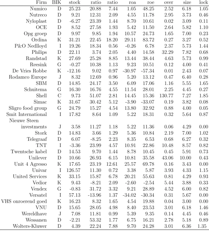
Table 2: Statistics per firm. The first column gives the name of the firm. The second column denotes the BIK code of the firm; see Table 1 for the description of these codes. Columns 3 to 7 give the average performance of each firm over time. ’Stock’ denotes the percentage growth of the stock price (stock return), ’p/e ratio’ is the price-earnings ratio (stock price divided by earnings per share), ’p/b ratio’ is the price-to-book ratio (stock price divided by equity per share), ’roa’ denotes the return on assets (in percentages) and ’roe’ denotes return on equity (in percentages). The eighth column gives the av-erage turnover in billions of euros. The last two columns give board characteristics: the size of the board (average number of board members) and the average number of interlocks per director.
p/e p/b turn- board
inter-firm BIK stock ratio ratio roa roe over size lock
Aalberts D 24.06 15.38 4.47 10.55 31.88 0.49 3.91 0.72 ABN Amro J 13.65 11.99 2.42 0.77 20.74 14.90 13.36 1.41 Acomo G 12.08 9.16 1.96 13.49 25.72 0.19 3.73 0.00 Aegon J 20.84 22.51 3.14 1.06 14.36 22.51 10.91 1.12 Ahold G 5.51 0.27 7.34 3.71 16.58 37.88 6.73 1.39 Akzo Nobel D 6.07 20.04 4.34 10.03 25.83 12.63 9.73 1.02 Alanheri G -5.00 53.02 0.75 0.31 1.33 0.13 3.00 0.15 AM F 7.07 11.05 1.79 9.45 16.64 1.56 5.36 0.43 Arcadis K 11.22 9.94 1.80 10.03 19.18 0.68 6.55 0.37 ASM International D 49.82 79.22 6.12 6.05 -3.66 0.50 4.36 0.92 ASML D 42.11 27.50 8.39 11.51 11.57 1.38 6.30 0.46 Athlon K 20.37 11.80 2.16 2.95 20.53 0.80 3.91 0.55 Ballast Nedam F 3.93 7.89 1.08 0.88 2.49 1.87 6.18 0.70 BAM F 16.72 5.31 1.52 5.26 19.46 2.74 6.55 0.55 Batenburg beheer F 4.38 8.69 1.54 13.85 18.54 0.11 2.91 0.24 Beterbed G 12.15 13.61 10.34 18.96 52.31 0.20 3.25 0.44 Boskalis F 8.78 10.77 1.76 8.54 19.06 0.86 5.45 1.26 Brunel K -0.76 32.10 2.63 14.69 16.04 0.23 3.25 0.31 Buhrmann G 0.62 58.29 1.12 2.29 4.57 7.56 7.55 1.56 Ten Cate D 7.34 5.32 1.07 6.00 7.53 0.62 5.55 0.84 LogicaCMG K 60.93 15.92 14.82 1.03 0.43 1.75 4.22 0.24 Coberco D 0.20 7.61 NA 6.50 12.94 4.32 11.43 0.21 Corio J 8.43 NA 1.03 5.19 9.76 0.19 5.91 0.73 Corus D -16.66 2.39 0.69 5.61 8.10 9.09 8.64 1.27
Crown van Gelder D 2.29 2.25 0.59 9.41 7.49 0.13 4.00 0.05
Table 2 – continued from previous page
p/e p/b turn- board
inter-Firm BIK stock ratio ratio roa roe over size lock
CSM D 4.98 14.15 4.59 13.06 41.37 2.57 6.36 1.19 CTAC K -11.12 22.64 5.91 17.00 33.80 0.02 2.71 0.43 Delft Instruments D 5.89 11.83 1.43 4.68 4.61 0.20 5.27 0.53 Dico international D -11.11 1.65 0.58 -13.70 -25.55 0.03 2.82 0.33 DOCdata D -9.25 11.60 1.35 4.39 5.35 0.09 3.13 0.44 Draka D 10.82 18.27 2.22 6.71 17.65 1.20 5.55 1.08 DSM D 9.87 10.34 1.09 7.68 17.17 6.49 7.82 0.57 Econosto D -10.28 21.83 2.50 1.60 -4.14 0.29 4.00 0.11 Elsevier D 3.76 -98.96 5.21 13.62 11.35 5.90 7.55 0.99 Eriks group G 6.63 24.15 1.57 12.52 17.34 0.30 3.00 0.00 Eurocommercial properties J 8.19 15.38 1.00 3.57 6.35 0.07 4.00 0.00 EVC International D 5.52 -2.09 0.49 -2.32 -18.10 1.06 4.10 0.13 Exact K -4.23 25.57 8.70 25.19 35.42 0.18 4.29 0.12 Exendis D -5.12 9.19 2.25 5.41 2.27 0.02 3.36 0.30 de Porceleyne Fles D 8.18 10.00 1.73 5.85 13.02 0.00 3.18 0.24 Fornix D 37.76 6.72 5.19 16.98 24.65 0.04 3.18 0.00 Fortis J 13.95 -147.55 2.81 9.09 11.55 1.79 10.80 0.16 Frans Maas I 2.11 9.38 1.67 5.74 12.00 0.82 4.55 0.50 Fugro K 27.57 13.24 3.60 10.68 32.41 0.67 5.73 0.61 Gamma Holding D 0.78 9.85 1.36 8.73 15.33 0.82 6.09 1.49 Getronics K 32.28 28.15 10.20 5.24 13.67 2.52 4.82 0.67 Grolsch D 0.30 16.69 2.96 14.87 17.61 0.24 6.00 1.07 Grontmij K 10.20 13.13 1.23 6.04 13.56 0.39 6.18 0.38 Hagemeijer G -9.37 16.12 3.43 4.90 11.60 6.17 5.91 0.85 Heijmans F 19.30 9.90 1.93 9.32 21.85 1.61 4.82 0.79 Heineken D 7.18 23.70 4.83 12.38 22.02 6.85 7.36 1.59 Hunter Douglas D 9.87 10.27 1.93 12.59 19.38 1.44 7.00 0.20 Imtech K 14.87 9.23 2.39 9.40 34.26 2.10 6.18 1.41 ING J 16.31 11.88 1.82 NA 18.37 9.29 11.45 1.06 Kas bank J 15.01 10.36 1.17 NA 14.17 0.10 7.09 0.06 Kendrion D -11.25 6.98 3.42 2.72 -3.68 0.73 3.64 0.17 KLM I 1.17 70.17 0.74 0.32 6.70 6.10 9.36 0.95 KPN I 7.27 14.54 2.68 1.73 -3.37 10.73 7.55 0.92 Van Lansschot J 4.81 13.43 2.27 NA 18.21 0.35 8.43 0.74 Macintosh Retail G 6.55 16.26 1.39 7.74 13.48 0.69 5.00 0.62 Magnus K -22.05 35.62 5.39 5.35 4.89 0.03 2.33 0.00
Van der Molen J 22.55 6.63 4.11 10.09 62.13 0.20 4.64 0.18
Nedap D 20.58 16.38 3.36 16.63 21.36 0.10 3.91 0.26
Nedschroef D 16.11 5.62 0.94 7.32 10.77 0.25 5.00 0.18
Table 2 – continued from previous page
p/e p/b turn- board
inter-Firm BIK stock ratio ratio roa roe over size lock
Numico D 25.23 20.88 7.44 1.05 48.25 2.52 6.18 1.05 Nutreco D 9.21 12.31 2.09 4.55 11.78 2.95 3.73 0.46 Nyloplast D -6.27 23.39 1.44 8.70 10.61 0.02 3.09 0.11 OCE D 8.52 27.58 1.93 5.42 11.50 2.64 5.82 1.10 Opg groep D 9.97 9.85 1.94 10.57 24.73 1.65 7.00 0.23 Ordina K 31.21 22.45 18.20 29.11 83.72 0.27 3.27 0.52 P&O Nedlloyd I 19.26 18.34 0.56 -0.26 6.78 2.37 5.73 1.44 Philips D 22.11 3.74 2.05 4.40 14.58 32.29 7.82 0.68 Randstad K 27.69 25.28 8.85 13.44 38.44 4.63 5.73 0.99 Reesink G -0.27 10.38 1.13 9.23 10.51 0.12 4.00 0.41 De Vries Robbe K -12.16 9.02 0.97 -30.97 -57.34 0.01 2.43 0.07 Rodamco Europe J 8.32 12.69 0.96 5.20 13.12 0.47 6.40 0.28 SBM D 14.85 24.17 3.50 6.09 17.06 1.16 5.55 1.65 Schuitema G 16.30 16.76 4.55 11.54 28.01 2.25 4.45 0.27 Shell C 9.73 51.07 2.81 14.45 15.36 130.77 7.27 1.85 Simac K 31.67 30.42 5.12 -3.90 -33.07 0.19 3.82 0.08
Sligro food group G 24.79 15.27 4.54 13.80 32.92 0.88 4.00 0.05
Smit International I 17.82 8.64 1.09 5.22 18.31 0.32 5.64 0.87 Nieuwe Steen investments J 3.58 11.27 1.18 5.22 11.36 0.06 4.29 0.00 Stork D 14.83 3.66 1.29 5.36 10.84 2.19 7.00 1.02 Telegraaf D 6.07 -8.25 2.23 8.35 6.53 0.68 6.27 0.32 TNT I -3.36 23.99 4.57 10.91 22.86 10.48 8.57 0.82 Twentsche kabel D 14.53 9.70 1.44 8.78 10.45 0.45 5.91 0.73 Unilever D 10.66 26.93 6.15 10.81 35.58 43.06 10.00 0.43 Unit 4 Agresso K 17.65 23.19 12.61 25.57 69.78 0.16 3.43 0.00 Univar I 126.57 11.30 0.72 3.38 5.87 3.93 4.33 1.15 United Services K 33.15 15.87 6.78 20.21 55.63 0.81 4.29 0.93 Vedior K 9.43 -8.21 2.09 -2.60 -2.54 5.44 3.88 0.33 Vendex G -0.83 31.72 3.32 9.21 28.89 4.52 6.00 0.82 Versatel I 57.13 -13.96 1.37 -34.02 -30.34 0.31 5.67 0.00 VHS onroerend goed K 16.23 8.32 1.65 4.54 19.88 0.04 3.00 0.00 VNU D 15.65 28.05 4.98 8.40 23.53 3.01 6.18 1.46 Wereldhave J 7.08 11.81 0.99 5.39 9.35 0.14 4.45 0.46 Wessanen D -2.21 53.32 1.77 6.75 16.21 2.78 5.18 0.89 Wolters-Kluwer D 4.39 22.24 7.88 9.70 24.28 3.01 6.36 1.35
Table 3: Statistics per year. The first column gives the year. Columns 2 to 6 give the average performance in each year. ’Stock’ denotes the percentage growth of the stock price (stock return), ’p/e ratio’ is the price-earnings ratio (stock price divided by earnings per share), ’p/b ratio’ is the price-to-book ratio (stock price divided by equity per share), ’roa’ denotes the return on assets (in percentages) and ’roe’ denotes return on equity (in percentages). The seventh column gives the average turnover in billions of euros. The last two columns give board characteristics: the size of the board (average number of board members) and the average number of interlocks per director.
year stock p/e ratio p/b ratio roa roe turnover board size interlock
1994 2.67 11.11 1.53 6.05 7.99 NA 6.18 0.69 1995 7.26 14.14 2.83 11.32 12.18 3.06 5.98 0.70 1996 45.38 17.54 3.61 9.90 22.42 3.34 5.77 0.66 1997 27.56 22.03 4.62 9.83 28.83 3.85 5.64 0.67 1998 1.02 25.82 5.56 10.27 26.09 3.57 5.63 0.79 1999 16.66 29.15 4.52 8.19 21.91 4.18 5.46 0.77 2000 1.65 25.65 3.50 5.91 18.59 5.52 5.59 0.73 2001 -13.97 20.86 2.40 3.73 6.05 5.61 5.60 0.72 2002 -27.72 12.23 1.69 1.12 -3.38 5.66 5.60 0.72 2003 36.32 19.32 2.00 2.84 8.97 5.42 5.49 0.69 2004 21.95 28.54 2.16 5.87 9.26 5.82 5.36 0.60
Table 4: Sample sizes for the five performance measures. stock return 734 price-earnings ratio 616 price-to-book ratio 722 return on assets 716 return on equity 734
Table 5: Summary statistics for each of the performance measure samples, where the sample sizes are given in Table 4. Each column corresponds to the sample of one of the (transformed) performance measures: the log of (1+ stock return/100), the logs of the price-earnings and price-to-book ratios, the return on assets (in percentages, no transformation applied) and the return on equity (in percentages, no transformation applied). The first panel gives the mean, the standard deviation (s.d.) and the median of the (transformed) performance measures itself. The second panel gives the same statistics on the number of interlocks per director. Panel three gives the same statistics on the turnover (in billions of euros) and the last panel gives the same statistics on the percentage growth of the turnover. Note that the columns of panels two, three and four thus concern different sample sizes.
stock return p/e ratio p/b ratio roa roe
mean -0.018 2.667 0.731 6.047 14.379 dependent s.d. 0.438 0.794 0.859 13.361 31.166 median 0.001 2.550 0.642 7.225 15.735 mean 0.638 0.668 0.638 0.638 0.638 interlock s.d. 0.552 0.560 0.554 0.555 0.551 median 0.500 0.571 0.536 0.500 0.571 mean 5.347 5.665 5.295 5.420 5.400 turnover s.d. 17.140 18.189 17.192 17.336 17.143 median 0.849 0.917 0.821 0.903 0.900 mean 10.527 11.927 10.925 10.427 10.614 growth turnover s.d. 33.980 28.160 33.899 34.267 33.709 median 5.950 8.060 6.210 5.850 5.940
Table 6: AIC’s of the different models. Each combination of performance measure and panel data model (FE, RE, BIK) is estimated in six different forms, that is, with interlocks incorporated linearly, quadratically and in a square root and both lagged and not lagged. This table gives for each combination of performance measure and panel data model the lowest and highest obtained AIC’s of the six different forms.
model lowest AIC highest AIC
FE 1.041 1.052
growth of stock price RE 1.177 1.206
BIK 0.895 0.898
FE 2.057 2.068
price-earnings ratio RE 2.123 2.135
BIK 2.402 2.403
FE 1.265 1.295
price to book ratio RE 1.515 1.542
BIK 2.299 2.310 FE 7.474 7.478 return on assets RE 7.532 7.537 BIK 7.531 7.547 FE 9.428 9.440 return on equity RE 9.458 9.470 BIK 9.639 9.650
Table 7: Estimation results on the performance measures log(stock return/100 + 1), log(price-earnings ratio) and log(price-to-book ratio), p-value in parentheses. The column ’model’ denotes which model is used (FE, RE or BIK model), which transformation of interlock is used (linear, quadratic or square root) and whether interlock is lagged. The column ’F-test’ gives the p-value of the F-test of joint significance of interlock and interlock-squared.
measure model interlock interlock2
F-test AIC
stock BIK, linear -0.004 (0.888) - - 0.896
BIK, quadr. -0.007 (0.930) 0.002 (0.968) 0.989 0.898
BIK, sq.root 0.000 (0.999) - - 0.896
BIK, linear, lag -0.009 (0.757) - - 0.896
BIK, quadr., lag -0.089 (0.268) 0.048 (0.285) 0.538 0.897
BIK, sq.root, lag -0.016 (0.653) - - 0.895
p/e ratio FE, linear -0.134 (0.200) - - 2.064
FE, quadr. 0.353 (0.137) -0.268 (0.023) 0.033 2.057
FE, sq. root -0.028 (0.839) - - 2.067
FE, linear, lag 0.038 (0.719) - - 2.067
FE, quadr., lag 0.285 (0.227) -0.134 (0.241) 0.471 2.068
FE, sq.root, lag 0.156 (0.257) - - 2.065
p/b ratio FE, linear -0.158 (0.016) - - 1.292
FE, quadr. -0.200 (0.169) 0.025 (0.743) 0.053 1.295
FE, sq. root -0.201 (0.014) - - 1.292
FE, linear, lag -0.311 (0.000) - - 1.265
FE, quadr., lag -0.401 (0.004) 0.053 (0.466) 0.000 1.267
Table 8: Estimation results on the performance measures return on assets and return on equity, p-value in parentheses. The column ’model’ denotes which model is used (FE, RE or BIK model), which transformation of interlock is used (linear, quadratic or square root) and whether interlock is lagged. The column ’F-test’ gives the p-value of the F-test of joint significance of interlock and interlock-squared.
measure model interlock interlock2
F-test AIC
roa FE, linear -1.035 (0.465) - - 7.476
FE, quadr. -0.403 (0.899) -0.365 (0.824) 0.747 7.478
FE, sq. root -1.410 (0.428) - - 7.475
FE, linear, lag -1.033 (0.465) - - 7.476
FE, quadr., lag 3.450 (0.265) -2.572 (0.104) 0.203 7.474
FE, sq.root, lag 0.544 (0.755) - - 7.476
roe FE, linear -4.193 (0.268) - - 9.439
FE, quadr. 2.797 (0.741) -4.033 (0.356) 0.353 9.440
FE, sq. root -2.294 (0.629) - - 9.440
FE, linear, lag -10.483 (0.005) - - 9.428
FE, quadr., lag -3.286 (0.689) -4.145 (0.325) 0.013 9.429
Table 9: Estimation results including a ’busyness’ parameter for performance mea-sures log(stock return/100 + 1), log(price-earnings ratio) and log(price-to-book ra-tio), p-value in parentheses. The column ’model’ denotes which model is used (FE, RE or BIK model), which transformation of interlock is used (linear, quadratic or square root) and whether interlock is lagged. The column ’F-test’ gives the p-value of the F-test of joint significance of interlock and interlock-squared.
measure model interlock interlock2
F-test ratio non-busy AIC
stock BIK, linear -0.011 (0.760) - - 0.192 (0.488) 0.898
BIK, quadr. -0.021 (0.794) 0.023 (0.662) 0.868 0.261 (0.414) 0.900
BIK, sq.root 0.013 (0.742) - - 0.179 (0.473) 0.898
BIK, linear, lag -0.017 (0.641) - - -0.096 (0.718) 0.898
BIK, quadr., lag -0.091 (0.263) 0.052 (0.308) 0.533 0.051 (0.866) 0.899
BIK, sq.root, lag -0.023 (0.577) - - -0.082 (0.731) 0.898
p/e ratio FE, linear -0.011 (0.923) - - 1.594 (0.030) 2.058
FE, quadr. 0.334 (0.159) -0.208 (0.094) 0.244 1.185 (0.124) 2.056
FE, sq.root 0.101 (0.486) - - 1.790 (0.009) 2.057
FE, linear, lag 0.094 (0.427) - - 0.747 (0.294) 2.068
FE, quadr., lag 0.270 (0.253) 0.105 (0.390) 0.504 0.520 (0.494) 2.070
FE, sq.root, lag 0.208 (0.149) - - 0.789 (0.237) 2.065
p/b ratio FE, linear -0.100 (0.178) - - 0.770 (0.107) 1.291
FE, quadr. -0.210 (0.149) 0.069 (0.380) 0.275 0.909 (0.071) 1.292
FE, sq.root -0.147 (0.089) - - 0.827 (0.063) 1.289
FE, linear, lag -0.283 (0.000) - - 0.380 (0.403) 1.266
FE, quadr., lag -0.412 (0.004) 0.083 (0.281) 0.000 0.557 (0.249) 1.267
Table 10: Estimation results including a ’busyness’ parameter for performance mea-sures return on assets and return on equity, p-value in parentheses. The column ’model’ denotes which model is used (FE, RE or BIK model), which transformation of interlock is used (linear, quadratic or square root) and whether interlock is lagged. The column ’F-test’ gives the p-value of the F-test of joint significance of interlock and interlock-squared.
measure model interlock interlock2
F-test ratio non-busy AIC
roa FE, linear -0.494 (0.763) - - 6.850 (0.508) 7.478
FE, quadr. -0.472 (0.882) -0.014 (0.994) 0.956 6.821 (0.534) 7.480
FE, sq.root -0.947 (0.617) - - 6.760 (0.479) 7.477
FE, linear, lag -0.214 (0.895) - - 10.340 (0.301) 7.477
FE, quadr., lag 3.354 (0.278) -2.279 (0.176) 0.397 5.362 (0.614) 7.476
FE, sq.root, lag 1.450 (0.434) - - 13.426 (0.147) 7.476
roe FE, linear -1.963 (0.652) - - 28.150 (0.303) 9.440
FE, quadr. 2.565 (0.762) -2.879 (0.533) 0.744 22.330 (0.439) 9.442
FE, sq.root 0.062 (0.990) - - 34.356 (0.174) 9.440
FE, linear, lag -9.069 (0.035) - - 17.785 (0.498) 9.430
FE, quadr., lag -3.460 (0.674) -3.585 (0.425) 0.079 10.036 (0.720) 9.432
Table 11: Estimation results including an upper class parameter for performance measures log(stock return/100 + 1), log(price-earnings ratio) and log(price-to-book ratio), p-value in parentheses. The column ’model’ denotes which model is used (FE, RE or BIK model), which transformation of interlock is used (linear, quadratic or square root) and whether interlock is lagged. The first column ’F-test’ gives the p-value of the F-test of joint significance of ’interlock’ and ’interlock-squared’, the second column ’F-test’ does the same for the ratio non-upper class.
measure model interlock interlock2
F-test ratio non-upper class ratio2
F-test AIC
stock BIK, linear 0.039 (0.503) - - 0.718 (0.204) 0.390 (0.299) 0.370 0.898
BIK, quadr. -0.068 (0.590) 0.059 (0.337) 0.504 1.195 (0.112) -0.729 (0.157) 0.233 0.899 BIK, sq.root 0.030 (0.652) - - 0.615 (0.276) -0.349 (0.381) 0.414 0.899 BIK, linear, lag 0.003 (0.953) - - 0.405 (0.494) -0.244 (0.535) 0.784 0.900 BIK, quadr., lag -0.215 (0.086) 0.119 (0.050) 0.146 1.372 (0.075) -0.935 (0.076) 0.202 0.897 BIK, sq.root, lag -0.028 (0.668) - - 0.445 (0.456) -0.310 (0.459) 0.755 0.900 p/e ratio FE, linear -0.146 (0.394) - - 1.701 (0.202) -1.217 (0.171) 0.390 2.067 FE, quadr. 0.393 (0.250) -0.292 (0.068) 0.131 -0.392 (0.823) 0.267 (0.824) 0.975 2.063 FE, sq.root 0.056 (0.775) - - 1.944 (0.135) -1.130 (0.221) 0.242 2.068 FE, linear, lag 0.057 (0.740) - - -0.129 (0.928) 0.134 (0.887) 0.979 2.074 FE, quadr., lag 0.526 (0.106) -0.259 (0.090) 0.225 -2.144 (0.249) 1.538 (0.219) 0.462 2.071 FE, sq.root, lag 0.266 (0.157) - - -0.374 (0.785) 0.468 (0.627) 0.674 2.070 p/b ratio FE, linear -0.211 (0.049) - - -0.007 (0.993) -0.113 (0.844) 0.807 1.297 FE, quadr. -0.317 (0.125) 0.061 (0.548) 0.120 0.440 (0.700) -0.424 (0.584) 0.712 1.299 FE, sq.root -0.235 (0.041) - - 0.536 (0.527) -0.418 (0.486) 0.775 1.296 FE, linear, lag -0.304 (0.004) - - -0.953 (0.291) 0.676 (0.255) 0.521 1.268 FE, quadr., lag -0.302 (0.119) -0.001 (0.989) 0.015 -0.964 (0.409) 0.683 (0.383) 0.680 1.271 FE, sq.root, lag -0.256 (0.019) - - -0.120 (0.891) 0.280 (0.650) 0.441 1.273
Table 12: Estimation results including an upper class parameter for performance measures return on assets and return on equity, p-value in parentheses. The column ’model’ denotes which model is used (FE, RE or BIK model), which transformation of interlock is used (linear, quadratic or square root) and whether interlock is lagged. The first column ’F-test’ gives the p-value of the F-test of joint significance of ’interlock’ and ’interlock-squared’, the second column ’F-test’ does the same for the ratio non-upper class.
measure model interlock interlock2
F-test ratio non-upper class ratio2
F-test AIC
roa FE, linear -3.122 (0.179) - - 29.227 (0.117) -24.907 (0.045) 0.078 7.473
FE, quadr. -8.914 (0.048) 3.318 (0.133) 0.131 53.671 (0.030) -41.948 (0.013) 0.026 7.472 FE, sq.root -4.437 (0.076) - - 38.240 (0.037) -31.015 (0.017) 0.042 7.470 FE, linear, lag 0.854 (0.708) - - 49.345 (0.012) -30.007 (0.021) 0.042 7.471 FE, quadr., lag 1.388 (0.745) -0.309 (0.882) 0.922 46.941 (0.066) -28.343 (0.099) 0.155 7.473 FE, sq.root, lag 2.132 (0.375) - - 45.911 (0.016) -26.773 (0.046) 0.024 7.469
roe FE, linear 4.681 (0.449) - - 99.999 (0.045) -49.529 (0.135) 0.057 9.435
FE, quadr. 3.131 (0.794) 0.888 (0.880) 0.742 106.538 (0.107) -54.088 (0.229) 0.086 9.438 FE, sq.root 5.136 (0.440) - - 87.708 (0.072) -42.665 (0.217) 0.034 9.435 FE, linear, lag -2.819 (0.642) - - 133.176 (0.012) -74.769 (0.031) 0.029 9.422 FE, quadr., lag -7.977 (0.484) 2.973 (0.593) 0.778 156.380 (0.022) -90.876 (0.048) 0.041 9.424 FE, sq.root, lag -2.602 (0.683) - - 141.306 (0.006) -78.915 (0.028) 0.004 9.422