Anti-windup control of nonlinear cascade systems
with particle swarm optimization parameter tuning
Fernando Serrano
Central American Technical University (UNITEC) Zona Jacaleapa, Tegucigalpa, Honduras
Josep M. Rossell
Dept. of Mathematics. Univ. Polit`ecnica de Catalunya (UPC) Avda. Bases de Manresa 61-73, 08242, Manresa, Spain
Abstract—Assuming that many physical models can be de-coupled, an anti-windup control scheme for nonlinear cascade systems is proposed. Taking into account that saturation appears frequently, in order to overcome this difficulty, an efficient control approach is developed. The paper is divided into two parts. Firstly, the design of a cascade control system with dynamic controllers in the inner and outer loops, considering the closed-loop stability in the controllers design with a suitable anti-windup compensator. Secondly, a PID cascade controller design in the inner and outer loop is presented, when the parameter tuning in both control schemes is done by particle swarm optimization (PSO). However, in this case, the implementation of an anti-windup compensator is not needed. Apart from the theoretical background, two numerical examples are shown to corroborate the provided results.
I. INTRODUCTION
Cascade control systems have been investigated since sev-eral decades ago. In the SISO linear case, as it is known, the controllers are tuned in sequence, first by tuning the inner loop and then the outer loop. Usually, the kind of controllers implemented are proportional-integral-derivative (PID). In re-cent years, the research about cascade control systems has been extended to the nonlinear case, considering that many physical systems such as mechanical, electrical, power systems and chemical systems can be controlled and stabilized by means of this approach. The design is possible because a decoupled system can be divided into an inner and an outer loop, improving the performance in comparison with single loop control techniques. In the literature, the research about this topic is limited but an example can be found in [1] where a cascade control system is designed for the stabilization of underactuated mechanical systems. Although the anti-windup control problem for cascade control systems has not been investigated extensively, there are interesting results in single loop anti-windup design. In [2], an anti-windup control design is developed for the control of Takagi-Sugeno systems and a reliable state feedback control of Takagi-Sugeno fuzzy systems with sensor faults can be seen in [3]. A control scheme for disturbance observer systems is provided in [4], dealing with the saturation torque. Other theoretical and applied studies have been presented in [5], where the results are implemented in single loop linear systems and the gain matrices are
This work was partially supported by the Spanish Ministry of Economy and Competitiveness under Grant DPI2015-64170-R (MINECO/FEDER)
computed by using linear matrix inequalities (LMI’s). Based on a linear approach, an anti-windup control scheme for an underwater vehicle is given in [6] and an anti-windup approach for nonlinear systems can be found in [7]. Other interesting works related to this topic are given in [8], [9], [10].
In this paper, an anti-windup control scheme is proposed for the stabilization of cascade nonlinear systems, which is developed in two parts. The first one is a dynamic controller implemented in the inner and outer loop. The closed-loop stability of the system is based on the theory stability of Lyapunov [11]. An anti-windup compensator is designed in order to reduce the unwanted effects of windup such as a poor performance or even instability. The second part is done by implementing PID controllers in the inner and outer loop but now without anti-windup compensation. In the first and second part of this study the gain matrices are tuned by particle swarm optimization [12], [13], [14], [15].
The paper is organized as follows: In Section II, the design of an anti-windup control scheme for cascade control systems, implementing dynamic controllers in the inner and outer loop, is developed. In Section III, a PID cascade control system design is presented by considering the input saturation but without anti-windup compensator. In Section IV, a PSO algorithm is supplied in order to tune the gain matrices for both approaches. Two numerical examples are given in Section V and the conclusions can be found in Section VI.
II. ANTI-WINDUP CASCADE DYNAMIC CONTROLLER DESIGN
This section is devoted to design an anti-windup controller for nonlinear cascade systems. This strategy implements dy-namic controllers in the inner and outer loops with gain matrices that help to improve the system performance. The controllers are tuned, as explained in Section IV, by a particle swarm optimization algorithm to reduce the integral square error, i.e. the difference between the reference variable and the output of the outer system. The same applies to the inner system. The main idea of this first approach is to design an appropriate anti-windup compensator to deal with the unwanted effects when saturation appears in the inner loop. Even when the gain matrices are tuned by a PSO algorithm, the closed-loop stability of the inner and the overall systems
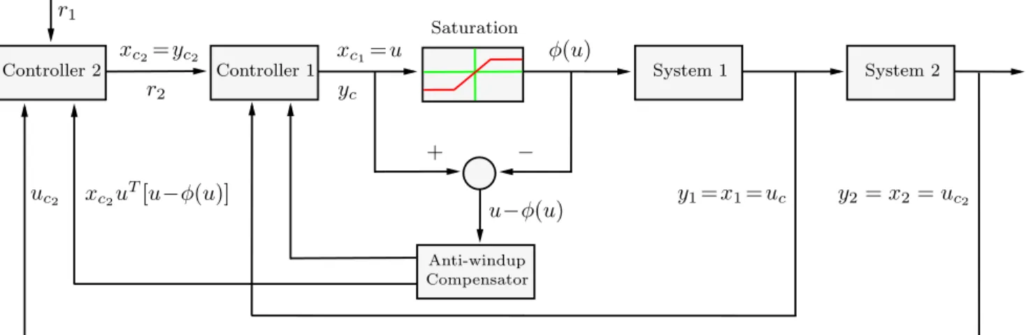
Controller 2 Anti-windup r1 xc2=yc2 xc1=u y1=x1=uc y2 =x2 =uc2 + − Controller 1 Saturation System 1 System 2 Compensator u−φ(u) xc2uT[u−φ(u)] φ(u) uc2 r2 yc
Fig. 1. Cascade anti-windup dynamic control scheme
are proved by the method of Lyapunov [11]. The obtained results are compared with the approaches given in [16], [17].
A. Inner loop dynamic controller design
Consider the cascade control dynamic scheme shown in Fig. 1. The inner loop system (system 1) is formed by
˙
x1(t) =−A x1(t) +f1(x1(t)) +φ(u(t)), y1(t) =x1(t) =uc(t),
(1)
whereA∈<n×n is an appropriate positive definite matrix due
to the inner loop system is minimum phase in order to facilitate the particle swarm optimization parameter tuning;x1(t)∈<nis
the state vector;f1(x1(t))a nonlinear vector function;φ(·)the saturation nonlinearity; u(t)∈<n the input vector; y1(t)
∈<n
the controller output and uc(t)∈<n is the controller input
vector. The inner loop controller is given by
˙
xc1(t) =−Kxc1(t) +r2(t)−[u(t)−φ(u(t))] +uc(t),
yc(t) =xc1(t) =u(t),
(2)
where K∈<n×n is a positive definite gain matrix with a
negative sign to make the closed-loop system of minimum phase type;xc1(t)∈<
nis the controller state vector;r2(t)
∈<n
the reference vector and u(t)−φ(u(t)) is the compensation term.
Before proving the closed-loop stability of the inner loop, the definition of sector condition is needed [1].
Definition 1:The sector condition for the saturation nonlin-earity is given by
uT(t)[u(t)−φ(u(t))]>0. (3) In the following theorem, the closed-loop stability of the inner loop is proved in order to obtain a stable controller by considering that the gain matrix K is tuned by means of a PSO algorithm, which is detailed in Section IV.
Theorem 1:There exists a gain matrixKfor the controller (2) such that the closed-loop of the inner loop is stable.
Proof:Consider the following storage function [11]:
V(x1(t), xc1(t)) =Vs(x1(t)) +σVsc(xc1(t)), (4)
withσ >0and where
Vs(x1(t)) = 1 2x T 1(t)x1(t), Vsc(xc1(t)) = 1 2x T c1(t)xc1(t) (5)
and the auxiliary input variable
v(t) =−f1(x1(t))−φ(u(t)). (6) Then, the system (1) becomes
˙
x1(t) =−A x1(t)−v(t) (7) and defining the input variable
w(t) =−r2(t)−uc(t), (8)
the system (2) can be written as
˙
xc1(t) =−K xc1(t)−w(t)−[u(t)−φ(u(t))]. (9)
Now, obtaining the first derivative of (4) along (7) and (9), yields ˙ V(x1(t), xc1(t))=−x T 1(t)Ax1(t)−xT1(t)v(t) −σhxTc1(t)Kxc1(t) +x T c1(t)w(t)+x T c1(t)[u(t)−φ(u(t))] i . (10)
From (1) and (2), x1(t)=y1(t) and xc1(t)=u(t). Then, the
equation (10) becomes in ˙ V(x1(t), xc1(t)) =−y T 1(t)Ay1(t)−y1T(t)v(t) −σ yTc(t)Kyc(t)+ycT(t)w(t)+uT(t) [u(t)−φ(u(t))] (11)
and using Definition 1 in (11) and considering that the system is zero state observable [7], i.e.yi(t)=0 impliesuci(t)=0 and
xi(t)=0, for i= 1,2, we obtain ˙
V(x1(t), xc1(t))≤0 (12)
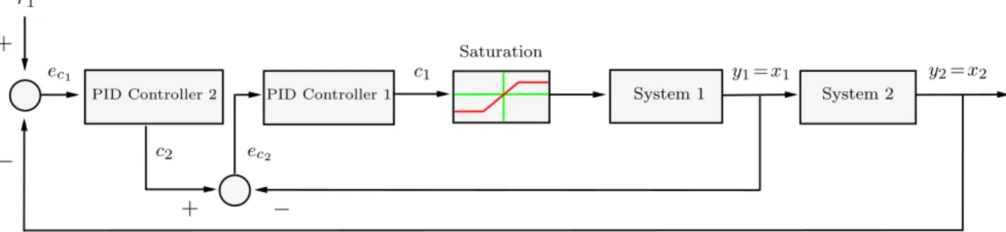
PID Controller 2 r1 ec1 ec2 y1=x1 y2=x2
+
−
PID Controller 1 Saturation System 1 System 2+
−
c2 c1Fig. 2. Cascade PID control scheme
B. Outer loop and overall dynamic controller design
Before deriving the outer loop controller and proving the overall closed-loop stability, it is necessary to make the following change of variables:
¯ x(t) = xT1(t), xTc1(t) T , ¯ u(t) = uT(t), φT(u(t)), rT2(t), uTc(t) T . (13)
The equivalent closed-loop system is
˙¯ x(t) = ¯Ax¯(t) + ¯f(¯x(t)) + ¯Bu¯(t), (14) with ¯ A= −A 0n 0n −K , f¯(¯x(t)) = f1(x1(t)) 0 , ¯ B= 0n In 0n 0n −In In In In , (15)
where In and 0n are the identity and the zero matrix of
appropriate dimensions, respectively. Now, consider the outer loop dynamic equation (system2) given by
˙
x2(t) =−A2x2(t) +f2(x2(t)) +u2(t), (16)
where A2∈<m×m is a positive definite matrix; x2(t)∈<m
is the state vector; f2(x2(t)) the nonlinearity vector and
u2(t)∈<m is the input vector. The overall closed-loop system
is obtained by selecting the augmented vectors
˜ x(t) = [xT1(t), xTc1(t), x T 2(t)]T, ˜ u(t) = [uT(t), φT(u(t)), r2T(t), uTc(t), uT2(t)]T. (17) Then, ˙˜ x(t) = ˜Ax˜(t) + ˜f(˜x(t)) + ˜Bu˜(t), ˜ y(t) =x2(t), (18)
where the output is given by
˜ y(t) = 0n 0n Im x1(t) xc1(t) x2(t) =x2(t) (19) withx2(t) =uc2(t)∈<
m the controller input,
˜ A= −A 0n 0m 0n −K 0m 0n 0n −A2 , f˜(˜x(t)) = f1(x1(t)) 0 f2(x2(t)) , ˜ B= 0n In 0n 0n 0m −In In In In 0m 0n 0n 0n 0n Im (20) and rewriting ˙˜ x(t) = ˜Ax˜(t)−v˜2(t) (21) with ˜ v2(t) =−f˜(˜x(t))−B˜u˜(t). (22) Consider the following outer loop dynamic controller: ˙ xc2(t) =−K2xc2(t)−r1(t)−xc2(t)˜z T (t) [u(t)−φ(u(t))]−uc2(t) =−K2xc2(t)−v2(t)−xc2(t)˜z T (t) [u(t)−φ(u(t))], (23) where xc2(t)∈<
m is the dynamic controller state vector,
K2∈<m×m the controller gain matrix, r1(t)∈<m the
refer-ence vector and defining
v2(t) =r1(t) +uc2(t),
yc2(t) =xc2(t),
(24)
where yc2(t)∈<
m is the controller output, together with an
extra output ˜ z(t) = 0n In 0m x1(t) xc1(t) x2(t) =xc1(t). (25)
Then, the following theorem can be stated.
Theorem 2:There exists a gain matrixK2for the controller
(23) such that the closed-loop of the outer loop (overall system) is stable.
Proof: Consider the storage function for the overall closed-loop system
V(˜x(t), xc2(t)) =Vs(˜x(t)) +σVsc(xc2(t)), (26)
withσ>0 and where
Vs(˜x(t)) = 1 2x˜ T(t)˜x(t), Vsc(xc2(t)) = 1 2x T c2(t)xc2(t). (27)
(23), we obtain ˙ V(˜x(t), xc2(t)) = ˜x T (t) ˜Ax˜(t)−x˜T(t) ˜v2(t) −σxT c2(t) h K2xc2(t)+v2(t)+xc2(t)u T(t)[u(t)−φ(u(t))]i. (28)
Then, from Definition 1, and considering that the system is zero state observable,
˙
V(˜x(t), xc2(t))≤0 (29)
is obtained and the closed-loop stability of the outer loop is ensured.
III. PIDCASCADE CONTROL SYSTEM DESIGN A PID cascade control system is formed by two parts: An inner loop PID controller [13] and an outer loop PID controller (see Fig. 2). In this case, it is not necessary to implement an anti-windup compensator because the gain matrices are tuned by the particle swarm optimization routine shown in the next section.
The PID controllers for the inner and outer loop are given by the following equations:
c1(t) =Kp1ec1(t) +Ki1 Z t 0 ec1(t)dt+Kd1e˙c1(t), c2(t) =Kp2ec2(t) +Ki2 Z t 0 ec2(t)dt+Kd2e˙c2(t), (30)
where c1(t)∈<n is the output controller 1; c2(t)∈<m the
output controller 2;ec1(t)=r1(t)−y2(t)the error variable for
the controller 1;ec2(t)=c2(t)−y1(t)the error variable for the
controller 2;Kp1, Ki1, Kd1∈<
n are the proportional, integral
and derivative gain matrices, respectively, for the controller 1 andKp2, Ki2, Kd2∈<
mfor the controller 2.
IV. PARTICLE SWARM OPTIMIZATION ROUTINE FOR CASCADE ANTI-WINDUP CONTROLLER DESIGN Particle swarm optimization routines have been recently implemented for the parameter tuning for PID’s and other controllers [12]–[15], [18]. In this study, the first step is to determine an anti-windup scheme for a cascade dynamic controller in order to find an appropriate controller and com-pensator ensuring the closed-loop overall stability. The gain matrices are found by using a PSO algorithm to minimize the integral squared error of the overall system [18], where
Fi(ei) = m
X
j=1
e2i(j)4j (31)
is the objective function that minimizes the error
ei(n) =r1(n)−y2(n)with the time difference4j. The PSO
algorithm that allows us to find the gain matrices K, K2 for
the dynamic controller and Kp1, Ki1, Kd1, Kp2, Ki2, Kd2 for
the PID controller scheme is given by
while (gbest> r1and gbest< r2... gbest< rn and j<100000)
for (int i=0; i<paramnum; i++)
V[i]=V[i] +c1(rand( ))(pbest[i]−c2(rand( )))(gbest−X[i]);
F=Objectivefunction(X) if (F[i]≤Fpbest[i]) pbest[i]=X[i]; Fpbest[i]=F[i]; if (F[1]≤Fgbest) gbest=X[i]; Fgbest=F[1];
where X is the particle position for the gain matrices component;V is the particle velocity;pbestandgbestare the best particle positions and F gbestis the final result obtained by the objective function.
V. NUMERICAL EXAMPLES
The following systems are implemented in two examples:
˙ x11(t) =−x11(t)−x12(t)+x311(t)+x11(t)x122 (t)+u1(t), ˙ x12(t) =−x12(t) + 2x11(t) +x412(t)x 2 11(t) +u2(t), (32) ˙ x21(t) =x321(t) +u1(t), ˙ x22(t) =x322(t)−x21(t)x22(t) +u2(t), (33)
where (32) and (33) will be the systems (1) and (2) for the example 1, and ˙ x11(t) =−x11(t)−0.0001x211(t) +u1(t), ˙ x12(t) =−x12(t)−0.0001x212(t) +u2(t), (34) ˙ x21(t) =−x21(t)−0.0001x221(t) +u1(t), ˙ x22(t) =−x22(t)−0.0001x2 22(t) +u2(t), (35) φ(x) = −19800 for x≤ −19800 x for −19800< x < 19800 19800 for x≥ 19800 (36)
where (34) and (35) will be the systems (1) and (2) for the example 2, with the saturation function given in (36).
A. Example 1: Dynamic controller experiment
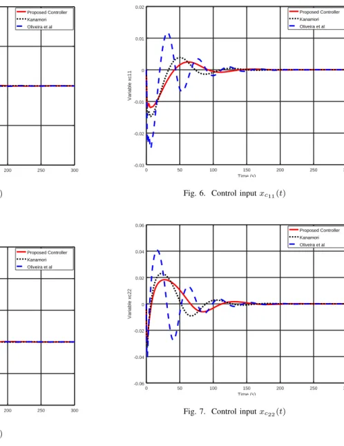
In this subsection, a numerical example to test the dynamic controller design is shown. The obtained results are compared with the results presented in [16], [17], considering that the strategies evinced in both studies are used in a cascade controller configuration. Fig. 3 and Fig. 4 depict the trajectories obtained by the variables x11(t)and x21(t), where the latest variable is the output of the overall closed-loop system when a reference is used to reach the origin or the equilibrium point. Note that these variables reach more efficiently the equilibrium point in comparison with the strategies given in [16] and [17], with less overshoot and faster response. The same occurs for the variable x22(t) shown in Fig. 5. In Fig. 6 and Fig. 7 the controller inputsxc11(t) andxc22(t) are presented and the
control effort generated by the control strategy is also smaller than the obtained in [16] and [17].
0 50 100 150 200 250 300 -0.01 -0.005 0 0.005 0.01 Time (s) Variable x11 Proposed Controller Kanamori Oliveira et al Fig. 3. Variablex11(t) 0 50 100 150 200 250 300 -0.1 -0.05 0 0.05 0.1 0.15 Time (s) Variable x21 Proposed Controller Kanamori Oliveira et al Fig. 4. Variablex21(t) 0 50 100 150 200 250 300 -0.03 -0.02 -0.01 0 0.01 0.02 Time (s) Variable x22 Proposed Controller Kanamori Oliveira et al Fig. 5. Variablex22(t) 0 50 100 150 200 250 300 -0.03 -0.02 -0.01 0 0.01 0.02 Time (s) Variable xc11 Proposed Controller Kanamori Oliveira et al
Fig. 6. Control inputxc11(t)
0 50 100 150 200 250 300 -0.06 -0.04 -0.02 0 0.02 0.04 0.06 Time (s) Variable xc22 Proposed Controller Kanamori Oliveira et al
Fig. 7. Control inputxc22(t)
B. Example 2: PID controller experiment
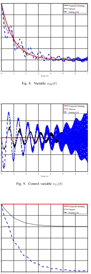
In this example, the PID controller gains are tuned by a PSO algorithm and the obtained results are compared with the ap-proaches shown in [19], [20], with the origin as the equilibrium point. The control approaches given in [19], [20] have been modified to operate in a cascade closed-loop configuration. The variablex22(t)is depicted in Fig. 8 and the desired final value has less oscillations and faster response in our case. Finally, in Fig. 9 and Fig. 10 the respective PID controller outputs c11(t) and c22(t) are shown and the control effort is smaller and with less oscillations, even when saturation is found in the input.
VI. CONCLUSIONS
Two anti-windup schemes for nonlinear cascade systems have been proposed and, when input saturation appears, the system performance is improved. The results represent a contribution in some physical systems such as mechanical, aeronautical, electrical, power and energy systems, considering that saturation is a common phenomenon affecting them.
0 1 2 3 4 5 6 7 -20 0 20 40 60 80 100 Time (s) Variable X22 Proposed Strategy Tahoun Huang et al Fig. 8. Variablex22(t) 0 1 2 3 4 5 6 7 -200 -100 0 100 200 Time (s) Variable C11 Proposed Strategy Tahoun Huang et al
Fig. 9. Control variablec11(t)
0 1 2 3 4 5 6 7 -30 -25 -20 -15 -10 -5 0 Time (s) Variable C22 Proposed Strategy Tahoun Huang et al
Fig. 10. Control variablec22(t)
[1] N. Mehdi, M. Rehan, F. M. Malik, A. I. Bhatti, and M. Tufail, “A novel anti-windup framework for cascade control systems: An application to underactuated mechanical systems,”ISA Transactions, vol. 53, no. 3, pp. 802 – 815, 2014.
[2] A. Nguyen, A. Dequidt, and M. Dambrine, “Anti-windup based dynamic output feedback controller design with performance con-sideration for constrained Takagi Sugeno systems,” Engineering Applications of Artificial Intelligence, vol. 40, pp. 76 – 83, 2015. [3] J. Dong and G-H. Yang, “Reliable state feedback control of T–
S fuzzy systems with sensor faults,” IEEE Transactions on Fuzzy Systems, vol. 23, no. 2, pp. 421 – 433, 2015.
[4] X. Gao, S. Komada, and T. Hori, “A wind-up restraint control of disturbance observer system for saturation of actuator torque,” in IEEE International Conference on Systems, Man, and Cybernetics, vol. 1, 1999, pp. 84–88.
[5] J. D. Silva and S.Tarbouriech, “Anti-windup design with guaranteed regions of stability: an LMI based approach,” inProceedings of the 42nd IEEE Conference on Decision and Control, vol. 5, 2003, pp. 4451–4456.
[6] J. P. Folcher, “LMI based anti-windup control for an underwater robot with propellers saturations,” inProceedings of the IEEE International Conference on Control Applications, vol. 1, 2004, pp. 32–37. [7] M. Z. Oliveira, J.M.G. Da Silva, D. Coutinho, and S. Tarbouriech,
“Anti-windup design for a class of multivariable nonlinear control systems: An LMI based approach,” in 50th IEEE Conference on Decision and Control and European Control Conference, 2011, pp. 4797–4802.
[8] D. Zhai and L. An and J. Li and Q. Zhang, “Fault detection for stochastic parameter-varying Markovian jump systems with applica-tion to networked control systems,”Applied Mathematical Modelling, vol. 40, no. 3, pp. 2368 – 2383, 2016.
[9] D. Zhai and L. An and J. Li and Q. Zhang, “Adaptive fuzzy fault-tolerant control with guaranteed tracking performance for nonlinear strict-feedback systems,”Fuzzy Set and Systems, vol. 302, pp. 80 – 100, 2016.
[10] D. Zhai and A-Y. Lu and J-H. Li and Q-L. Zhang, “Simultaneous fault detection and control for switched linear systems with mode-dependent average dwell-time,”Applied Mathematics and Computa-tion, vol. 273, pp. 767 – 792, 2016.
[11] W. Haddad and V. Chellaboina,Nonlinear Dynamical Systems and Control: A Lyapunov Based Approach. Princeton Press, 2008. [12] H. Gao and W. Xu, “Particle swarm algorithm with hybrid mutation
strategy,”Applied Soft Computing, vol. 11, no. 8, pp. 5129 – 5142, 2011.
[13] M. I. Menhas, L. Wang, M. Fei, and H. Pan, “Comparative perfor-mance analysis of various binary coded PSO algorithms in multi-variable PID controller design,” Expert Systems with Applications, vol. 39, no. 4, pp. 4390 – 4401, 2012.
[14] L. Wang, X. Fu, Y. Mao, M.I. Menhas, and M. Fei, “A novel modified binary differential evolution algorithm and its applications,” Neurocomputing, vol. 98, pp. 55 – 75, 2012.
[15] Y. Wang, B. Li, T.Weise, J. Wang, B. Yuan, and Q. Tian, “Self-adaptive learning based particle swarm optimization,” Information Sciences, vol. 181, no. 20, pp. 4515 – 4538, 2011.
[16] M. Kanamori, “Anti-windup adaptive law for Euler–Lagrange sys-tems with actuator saturation,”IFAC Proceedings, vol. 45, no. 22, pp. 875 – 880, 2012.
[17] M. Z. Oliveira, J. M. Gomes da Silva, D. F. Coutinho and S. Tarbouriech, “Anti-windup design for a class of nonlinear control systems,” IFAC Proceedings Volumes, vol. 44, no. 1, pp. 13432 – 13437, 2011.
[18] F. E. Serrano and M.A. Flores, “C++ library for fuzzy type-2 controller design with particle swarm optimization tuning,” IEEE CONCAPAN 2015, Tegucigalpa, Honduras, 2015.
[19] A. H. Tahoun, “Anti-windup adaptive PID control design for a class of uncertain chaotic systems with input saturation,”ISA Transactions, vol. 66, pp. 176 – 184, 2017.
[20] C. Q. Huang, X. F. Peng and J. P. Wang, “Robust nonlinear PID controllers for anti-windup design of robot manipulators with an uncertain Jacobian matrix,”Acta Automatica Sinica, vol. 34, no. 9, pp. 1113 – 1121, 2008.