Munich Personal RePEc Archive
Growth in a Cross-Section of Cities:
Location, Increasing Returns or Random
Growth?
González-Val, Rafael and Olmo, Jose
18 June 2014
Online at
https://mpra.ub.uni-muenchen.de/56732/
Growth in a Cross-Section of Cities: Location,
Increasing Returns or Random Growth?
Rafael González-Val1
Jose Olmo2
1
Universidad de Zaragoza & Institut d'Economia de Barcelona (IEB) 2
University of Southampton
Abstract
This article analyses empirically the main existing theories on income and population city
growth: increasing returns to scale, locational fundamentals and random growth. To do this
we consider a large database of urban, climatological and macroeconomic data from 1,173
US cities observed in 1990 and 2000. The econometric model is robust to the presence of
spatial effects. Our analysis shows the existence of increasing returns and two distinct
equilibria in per-capita income and population growth. We also find important differences
in the structure of productive activity, unemployment rates and geographical location
between cities in low income and high income regimes.
Keywords: threshold tests, locational fundamentals, multiple equilibria, random growth
1. Introduction
There are differences in the growth rates of cities. It is evident that some cities (or regions)
are more productive than others, or attract more population, depending on certain
circumstances that vary over time. Several explanations have been proposed to try to
explain these differentiated behaviours. Following Davis and Weinstein (2002), these
theoretical explanations can be grouped into three main theories: the existence of increasing
returns to scale, the importance of locational fundamentals and the absence of both (random
growth).
To accommodate these different theories we propose a new econometric model
robust to the presence of spatial effects. Each of these models – random growth, locational
fundamentals and increasing returns to scale – are identified with a different set of
explanatory factors that describes the effects of the variables on per-capita income and
population growth. The locational fundamentals model is extended to consider
socioeconomic variables such as human capital and the structure of productive activity in
the relevant location. To assess the relative merits of the different empirical models behind
the theories, we propose multiple regression analysis and likelihood ratio tests. These tests
allow us to assess the overall significance of each model and the incremental gains of using
richer models that jointly consider different sets of variables, such as locational plus
socioeconomic fundamentals or locational plus lagged per-capita income. The existence of
increasing returns in per-capita income and population growth are assessed using a
cross-sectional threshold nonlinearity test. This nonlinear model enables us to test for the
presence of multiple growth regimes, which is one of the core topics in urban and regional
economics; one of the advantages of our procedure is that we can identify the threshold
value.
We consider a large database of urban, climatological and macroeconomic data
from 1,173 US cities observed in 1990 and 2000. Our results provide evidence of
increasing returns to scale on both per-capita income and population growth. The
econometric methodology is complemented with spatial tests to determine the statistical
importance of the spillover effects between neighbouring locations and two spatial
regression models to assess the marginal effects of these neighbouring locations on
The article is structured as follows. The next Section reviews the related literature.
Section 3 sets out the econometric framework. Section 4 discusses the different hypothesis
tests of interest. Section 5 discusses the empirical results for a database containing 1,173
US cities and the last Section concludes.
2. Related literature
Davis and Weinstein (2002) group the traditional theoretical explanations of urban growth
into three main theories: the existence of increasing returns to scale, the importance of
locational fundamentals and the absence of both (random growth).
The first theory is supported by the theoretical models of the New Economic
Geography (NEG). These models often display nonlinear behaviours and multiple
equilibria as a consequence of their basic assumptions (mobile factors, transport costs,
centrifugal and centripetal forces, etc.), which are very different from the classic
framework. The literature on urban increasing returns, also known as agglomeration
economies, is wide (see the meta-analysis by Melo et al., 2009). The traditional Marshallian
sources of external economies of scale are labour market pooling, input sharing and
knowledge spillovers. Duranton and Puga (2004) provide an alternative perspective,
namely that agglomeration economies could be driven by sharing, matching or learning
mechanisms. In addition, there is also evidence that other factors contribute to
agglomeration, such as home market effects, consumption opportunities and rent-seeking
(see the survey by Rosenthal and Strange, 2004).
In the economic literature, locational fundamentals are considered to be
geographical factors linked to the physical landscape, such as temperature, rainfall, access
to the sea, the presence of natural resources or the availability of arable land. Random
growth models usually assume that these characteristics are randomly distributed across
space, but actually they are not. From a physical geography perspective, factors such as
mineral resources and nice weather are clearly concentrated in certain areas. Several studies
find a significant influence of these characteristics on the development of some particular
regions. For example, the nearby deposits of coal, iron ore and limestone as well as the
extensive network of natural waterways and deep water sea and river ports contributed to
regions (Berry and Kasarda, 1977). Fernihough and O’Rourke (2014) also find that coal
had a strong influence on city population; according to their estimates coal explains at least
60% of the growth in European city populations from 1750 to 1900.
Nevertheless, although locational fundamentals may have played a crucial role in
early settlements, one would expect that their influence decreases over time. However,
empirical studies demonstrate that their important influence in determining agglomeration
remains. For the case of the United States, Ellison and Glaeser (1999) state that natural
advantages, such as the presence of a natural harbour or a particular climate, can explain
about 20% of the observed geographic concentration. Glaeser and Shapiro (2003) find that
in the 1990s people moved to warmer, dryer places, while Rappaport (2007) explains that a
large proportion of weather-related movement seems to be driven by an increased valuation
of nice weather as a consumption amenity.
Random growth theories are based on stochastic growth processes and probabilistic
models. The most important models are those presented by Champernowne (1953), Simon
(1955) and, more recently, Gabaix (1999). In the case of population growth, these models
are able to reproduce a empirical regularity well-known in urban economics: Gibrat's law
(or the law of proportionate growth). For the case of the US, several works statistically
accept the fulfilment of Gibrat’s law, whether at the level of places (Eeckhout, 2004;
González-Val, 2010) or metropolitan areas (Ioannides and Overman, 2003). In contrast to
these studies, Black and Henderson (2003) reject Gibrat’s law, using a different dataset of
metro areas in the US. Michaels et al. (2012) use data from Minor Civil Divisions and
counties to track the evolution of populations across both rural and urban areas in the US
from 1880 to 2000, finding that Gibrat’s law is a reasonable approximation for population
growth only for the largest units.
However, recent studies argue that empirically random growth can only hold as a
long-run average; Gabaix and Ioannides (2004) point out that “the casual impression of the
authors is that in some decades, large cities grow faster than small cities, but in other
decades, small cities grow faster.” This size-dependent growth would rebut random growth
in the short-term, but random growth theory would still be important from a long-term
perspective, because the influence of other factors such as locational fundamentals and
random growth models could be a combination of weak size-dependence and decaying
impact of locational fundamentals over time (because of advances in transportation and
communication technology) or random changes in the importance of each fundamentals
(e.g. in the case of weather).
While there are many studies of each of these theories, the literature on alternative
approaches is scant; only Davis and Weinstein (2002, 2008) and Bloom et al. (2003) adopt
such a broad perspective. The first authors support a hybrid theory in which locational
fundamentals establish the spatial pattern of relative regional densities, but increasing
returns help determine the degree of spatial differentiation in Japanese cities. Similarly,
Bloom et al. (2003) study the influence of climatological and geographical variables on
growth at a country level. These authors develop a Markov regime-switching model to
analyse whether locational fundamentals have additional explanatory power to describe
per-capita income growth compared with nonlinear models based on lagged per-capita
income. Finally, Davis and Weinstein (2008) develop a threshold regression framework for
distinguishing the hypothesis of unique versus multiple equilibria and apply it to the Allied
bombing of Japan during World War II, finding evidence against multiple equilibria.
Bosker et al. (2007) replicate this analysis for the bombing of Germany during World War
II and their results support a model with two stable equilibria.
3. Econometric Methodology: Estimation and Testing
The structural factors that contribute to city income include consumption, investment, trade
and local government expenditure. All these variables depend on a set of socioeconomic
and geographical variables that determine the economic size of a city. These variables
include literacy variables such as schooling, socioeconomic variables such as productive
structure or unemployment rate and geographical and environmental variables such as
temperature or climate. Our interest is in studying the influence of these explanatory
variables on aggregate measures of wealth and population growth. Among the several
potential indicators for economic activity we choose two different dependent variables at
the city level: population and per-capita income. Both of them are second nature variables
closely linked (higher per-capita income stimulates migration), but they give different
information. Although both variables are assumed to capture many agglomeration
population is a measure of urban concentration and a proxy for urban amenities and
potential congestion costs (Melo et al., 2009), while income is a more direct measure of
city’s productivity. Empirical studies usually consider only one of them; one exception is
Roos (2005), who considers these two second-nature variables and develops a stepwise
procedure to infer the unobservable effect of first nature for Germany. Chasco et al. (2012)
adapt this framework to allow spatial effects.
For both aggregate response variables, we formulate two working hypotheses
defined by a linear and a nonlinear model on a cross-sectional two-period model. Let yio
denote the initial log per-capita income and yif the corresponding variable in the terminal
period for city i, while xio is a vector of socioeconomic and geographical indicators. We
will assume throughout that the relationship between initial conditions and the response
variables measuring growth is constant across cities in the sample. Thus, for per-capita
income growth the linear model is
, '
2 1
0 io io i
i y x
y =γ +γ +γ +ε
Δ (1)
with Δyi = yif −yio, γ0 the intercept of the model, (γ1,γ2') a vector of parameters
describing the marginal effect of the regressors and i an independent and identically distributed (iid) error term with constant variance. The study of population growth follows
similarly; let lio be the initial level of population (in logs) and lif the corresponding
variable in the terminal period. A suitable regression equation for measuring population
growth is
,
2 1 0
∗
′ +
+ + =
Δli η ηlio η xio εi (2)
with Δli =lif −lio and i∗ a mean zero iid error term with constant variance; 0 is the
intercept and 1and 2 are the parameters that describe the marginal effect of the
explanatory variables. The economic foundations for equation (2) can be found in the
theoretical framework of urban growth put forward in Glaeser et al. (1995). This is a model
of spatial equilibrium similar to the Roback (1982) model, where the relationship between
population growth and initial characteristics is determined by changes in demand for some
initial characteristic on productivity growth. The negative values of γ1 and η1 in equations
(1) and (2) indicate convergence. However, the existence of a spatial equilibrium does not
necessarily imply the same equilibrium city size and thus growth convergence across
cities.1 In Henderson’s (1974) seminal system of cities model (and in many of the
subsequent models) all cities are fully specialised in equilibrium and only the cities with the
same specialisation must be of the same size (Combes et al., 2005). Nevertheless, other
theoretical frameworks combine diversified and specialized cities (Duranton and Puga,
2001) and in equilibrium all the cities of the same type are of the same size.
These equations correspond to the well-known expression of the conditional
-convergence (Evans, 1997; Evans and Karras, 1996). Several theoretical economic growth
models can produce these equations at the state, county or region level. For a neoclassical
growth model, see Barro and Sala-i-Martin (1992). In particular, the nonlinear alternative to
(1) is motivated by the interest in macroeconomics and the empirical growth literature in
determining the existence of unique or multiple equilibria in per-capita income growth2.
Thus, theoretical papers on the existence of convergence clubs or conditional convergence
are, for example, Baumol (1986), De Long (1988) and Quah (1997). In our framework, the
nonlinear alternative, assuming the presence of at most two regimes in per-capita income, is
, '
) (
)
( 12 2
11
0 io io io io io i
i y I y u y I y u x
y =γ +γ ≤ +γ > +γ +ε
Δ (3)
with I an indicator variable taking the value of one when the argument is true and zero
otherwise. For γ11 <γ12 <0, the model describes the existence of increasing returns to
scale for values of initial per-capita income greater than a threshold value u defined on a
compact space U ∈ R, because in that situation the cities with a higher initial per-capita
income grow at a higher rate. This can be better observed if (3) is rewritten instead as
, ' ) ( ) 1 ( ) ( ) 1
( 11 12 2
0 io io io io io i
if y I y u y I y u x
y =γ + +γ ≤ + +γ > +γ +ε (3’)
1 We acknowledge one anonymous referee for suggesting this point. 2
In equilibrium (E
[ ]
εi =0) this model yields two different balanced growth paths. Inthe lower regime, per-capita income in equilibrium is equal to (1) 0 2 11
' io
if
x
y γ γ
γ +
= − and in the
upper regime the per-capita income in equilibrium is (2) 0 2 12 ' . io if x
y γ γ
γ +
= − From these
expressions and assuming that γ0+γ2'xio >0, it is not difficult to see that
(1) if
y < yif(2)if
0
12 11 <γ <
γ . This leads to two different city sizes for each growth path, but it should be
noted that for cities within each growth regime convergence takes place. While some NEG
models feature a location pattern that can only lead to ‘bang-bang’ outcomes (a symmetric
equilibrium with all the regions completely symmetrical or a corner one with all mobile
agents concentrated in one of the regions), our specification allows for the more realistic
result of partial agglomeration, fully consistent with others NEG models (see Pflüger and
Südekum, 2008).
Our model extends the study of Durlauf and Johnson (1995) by providing a formal
procedure for dividing the sample. Thus, this approach is different from those proposed in
previous empirical studies of growth convergence clubs, such as the regression tree analysis
used by Durlauf and Johnson (1995) and the predictive density of the data used by Canova
(2004) to identify different clusters of countries or regions. The analogue of equation (3)
for measuring nonlinearities in population growth is obtained by replacing the variable yi
with li in the preceding expression (see equations (6) and (7)). The vector xo controls for
the effect of socioeconomic and geographical (locational) fundamentals.
A further robustness check to measure the impact of these factors on the response
variables is to consider spatial statistical analysis. In a first step, we implement spatial
hypothesis tests such as the Lagrange multiplier and Moran’s I tests (see Moran, 1950;
Anselin, 1988) to assess the spillover effects between neighbouring locations in the
residuals of the above regression models. In a second step, we estimate a spatial error
model and a spatial autoregressive model with the aim of explicitly considering the impact
of neighbouring locations on per-capita income and population growth. In this context, the
spatial error model extends model (3) by considering an error variable that satisfies
, v W +
=λ ε
with λ <1 being a parameter that reflects the effect of the residuals of neighbouring
variables on the residual of location i, W a weighting matrix that measures the distances
between the different locations and vi an iid random variable that describes the error of the
regression model. There exist different possibilities for choosing W; we consider a matrix
obtained from the coordinates (longitude and latitude) of the locations in order to construct
the Euclidean distance between the cities in the empirical analysis. The spatial
autoregressive model considers the following econometric specification:
, )
( )
( 12 2
11
0 i io io io io io i
i W y y I y u y I y u x
y =γ +ρ Δ +γ ≤ +γ > +γ +ε
Δ (5)
with ρ <1 measuring the effect on the response variable of per-capita income growth in
neighbouring cities. Previous studies estimate conditional or unconditional -convergence
models allowing for spatial effects. Fingleton and López-Bazo (2006) survey the literature
on empirical growth models with spatial effects and provide theoretical foundations for the
linear specification of both spatial models based on two growth models with across-region
externalities due to knowledge diffusion. Beaumont et al. (2003) also estimate a
-convergence model with spatial effects, allowing for different spatial regimes. They define
two different convergence clubs using Exploratory Spatial Data Analysis (a Moran
scatterplot) considering a sample of 138 European regions over the period 1980–1995.3
Therefore, the main difference between previous studies and our method is the procedure
for dividing the sample. The threshold parameter u is estimated by the minimization of the
concentrated sum of squared residuals Sˆ
( ) ( ) ( )
u =eu ′eu with e( )
u being the residual of thecorresponding regression model for u fixed (see Hansen, 1997).
The estimation of these models is complex and follows different techniques
depending on the regression model assumed. Thus, models (1) and (2) can be estimated by
ordinary least squares, and standard asymptotic inference results hold. Model (3) is
nonlinear and depends on a prior estimation of the threshold value u. Once the threshold
value has been estimated, OLS methods can be applied to estimate the remainder of the
and bootstrap methods that approximate the finite-sample distribution of the supremum of
Chi-squared tests. Finally, the estimation of spatial models is also cumbersome and needs
to be carried out using maximum likelihood techniques under the assumption that the error
variables are normally distributed. Inference follows from applying well-known results for
maximum likelihood estimation methods.
4. Testing the three leading theories
The above models allow us to derive hypothesis tests for each of the leading hypotheses in
the analysis of cross-sectional city growth: increasing returns, random growth and
socioeconomic and locational fundamentals. For completeness, we also analyse the
existence of increasing returns to scale in population growth and the explanatory power of
the regressors outlined above.
4.1. Per-capita Income Growth
The first hypothesis under study is the existence of increasing returns to scale. Under
increasing returns to scale, the accumulation of output beyond a threshold u makes cities
more productive4; thus, per-capita income growth is endogenous. This hypothesis can be
tested using several of the above regression specifications. In particular, for models (3) and
(5), the hypothesis of interest can be expressed as H0,IRS : γ11 =γ12 vs.
HA,IRS :11 ≠ 12. The differences between both specifications lie on the inclusion or not of spatial effects in the regression equations. The existence of these effects is determined by
applying the Lagrange multiplier and Moran’s I tests to the residuals of the regression
equation (3).
The second hypothesis of interest is to assess the statistical significance of the
socioeconomic and locational fundamentals variables. In order to be robust to the existence
of increasing returns in per-capita income and spatial effects, we propose testing the
3
There are important differences between Beaumont et al. (2003)’s data and our sample. Their sample size is 9 times smaller than ours and they consider regions from different countries, while our sample includes cities from only one country.
4 This is a macroeconomic approach to increasing returns. However, some of our exogenous variables, i.e.
hypothesis H0,L : γ2 =0 vs. HA,L : γ2 ≠0 in model (5). One of the few and
pioneering studies concerned with the impact of locational fundamentals is Bloom et al.
(2003). These authors are interested in modelling the presence of nonlinearities in
per-capita income growth from country-level data using a model that incorporates
climatological and geographical variables. They propose a Markov regime-switching model
in which the probabilities that determine the change of regime depend on these
environmental (locational fundamentals) variables.
The last competing theory under analysis is that of random growth, namely, that no
explanatory variable helps systematically explain per-capita income growth. The null
hypothesis in model (3) is H0,R : γ11 =γ12 =γ2 =0. The reader should note that the
restriction 0γ11 =γ12 = is the key assumption of the random growth hypothesis. This is
because random growth implies that city growth rates are independent of initial city size.
By estimating model (5) instead, this hypothesis can be tested under the implicit presence
of spatial effects from neighbouring locations. A stronger version of the random growth
theory assumes that H0,R : γ11 =γ12 =γ2 =λ=0 or alternatively, for the spatial
autoregressive model, that H0,R : γ11 =γ12 =γ2 =ρ =0. Under the null hypothesis,
per-capita income growth is a random variable independently distributed across cities.
4.2. Population Growth
Similar tests can be carried out to gauge the empirical relevance of the above models in
city population growth. The object of interest is to assess whether population growth in US
cities is endogenous or exogenously determined by the set of socioeconomic and locational
fundamentals discussed earlier. By accommodating the existence of spatial effects, we
robustify the methodology in order to consider the spillover cross-border effects that come
from neighbouring locations.
The empirical analysis in the next section focuses on the spatial error model
, )
( )
( 12 2
11
0 io io io io io i
i l I l l I l x
l =η +η ≤ν +η >ν +η +ε
Δ (6)
with ε =λWε+v and λ <1 describing the spatial relationship between the residuals of
the nonlinear model; and on the spatial autoregressive model
, )
( )
( 12 2
11
0 i io io io io io i
i W l l I l l I l x
l =η +ρ Δ +η ≤ν +η >ν +η +ε
Δ (7)
with ρ <1 measuring the effect on the response variable of the growth in population in
neighbouring locations.
5. Empirical Results
This section illustrates the above econometric models and tests using data from all US cities
with more than 25,000 inhabitants in 2000 (1,173 cities).5 The dataset includes urban,
climatological, locational and macroeconomic variables on all these 1,173 cities. This
sample represents 41.34% of the total US population in this year, and 52.33% of the total
urban population.
5.1. Data
The data came from the censuses for 1990 and 2000 (see Appendix 1 for the details of the
data sources). We identified cities as what the US Census Bureau calls “incorporated
places”. The US Census Bureau uses the generic term incorporated place to refer to a type
of governmental unit incorporated under state law as a city, town, borough or village. They
are administratively defined “legal” cities; these places have been used recently in the
empirical analyses of American city size distribution (Eeckhout, 2004; González-Val, 2010;
Ioannides and Skouras, 2013). These cities may occupy a variety of spatial locations in the
territory, being either in the core or the periphery or at different distances of more or less
large metropolitan areas. In the US, to qualify as a metropolitan area a central city of
50,000 or more inhabitants is needed. Thus, although our cities may occupy very different
relative positions in the urban space of metropolitan areas, many of the selected
incorporated places that have more than 25,000 inhabitants are the central cities of a
metropolitan area.
5 There are 141 cities in our sample below the 25.000 inhabitants in 1990. As the sample is defined according
US urban growth has also been analysed using other geographical units: counties
(Beeson et al., 2001), minor civil divisions (Michaels et al., 2012), metropolitan areas
(Dobkins and Ioannides, 2001; Black and Henderson, 2003; Ioannides and Overman, 2003)
and urbanised areas (Garmestani et al., 2008). However, researchers usually choose
between two basic alternatives: administratively defined cities (incorporated places) and
metropolitan areas6. Both units have advantages. As Glaeser and Shapiro (2003) indicate,
metro areas represent urban agglomerations, covering huge areas that are meant to capture
labour markets. Metropolitan areas are attractive because they are more natural economic
units, while legal cities are political units that usually lie within metropolitan areas, and
their boundaries make no economic sense. However, certain factors, such as human capital
spillovers, are thought to operate at a very local level (Eeckhout, 2004). The economic area
of influence of labour markets and large infrastructure projects such as airports exceeds the
boundaries of single legal cities, while the geographical influence of factors such as public
services (schools, public transportation, etc.) and local externalities is more reduced.
Finally, the population of incorporated places is almost entirely urban, 94.18% in 2000,
compared with 88.35% of urban population in metropolitan areas.
One important limitation of incorporated places is the spillover effect or contagion
effect between neighbouring localities, which can influence the urban growth process. We
use spatial econometrics to deal with this issue. Moreover, the geographic boundaries of
census places can change between censuses. As in Glaeser and Shapiro (2003), we address
this issue by controlling for change in land area. We acknowledge that this control may not
be appropriate because it is also an endogenous variable that may reflect the growth of the
city, nevertheless, none of our results change significantly if this control is excluded.
Moreover, we also eliminate incorporated places that either more than doubled land area
(37 cities) or lost more than 10% of their land area (five cities). This correction eliminates
42 extreme cases where the city in 1990 is something very different from the city in 2000.
The explicative variables chosen are similar to those reported in other studies on city
growth in the US and city size, and correspond to the initial 1990 values. The influence of
If we consider all the incorporated places with 25,000 or more inhabitants in 1990 according to the US Census Bureau only 10 out of these 1,077 cities fall below the 25,000 inhabitants in 2000.
6
some of these variables on determining city size has been empirically illustrated in other
studies such as Glaeser et al. (1995) or Glaeser and Shapiro (2003). Our aim is to introduce variables to control for some of the already known empirical determinants of city growth
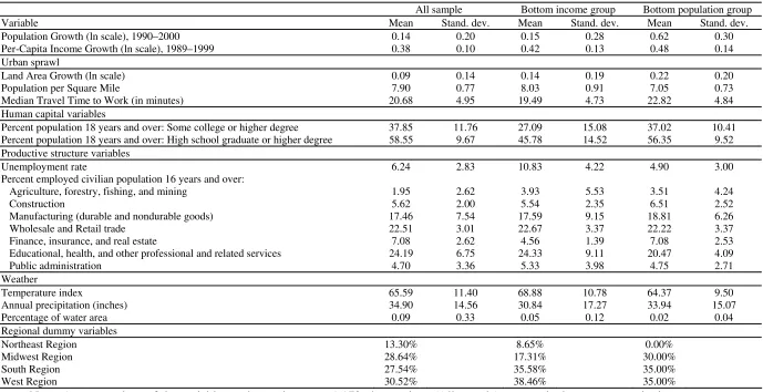
(human capital, density, weather). Table 1 presents the variables, which can be grouped
into four types: urban sprawl variables, human capital variables, productive structure
variables and weather variables.
Urban sprawl variables aim to reflect the effect of city size on urban growth. For
this, we use population density, growth in land area from 1990 to 2000 (as a control for
boundary changes) and the variable median travel time to work, which represents the
commuting cost borne by workers. Commuting time is endogenous and depends in part on
the spatial organisation of cities and location choice within cities. The median commuting
time may reflect traffic congestion in larger urbanised areas as well as the size of the city in
less densely populated areas, or the remoteness of location for rural towns; in other words,
the idea that as a city's population increases, so do the costs in terms of individuals’ travel
time to work.
Regarding human capital variables, many studies demonstrate the influence of
human capital on city size, as cities with better educated inhabitants tend to grow more. For
example, Glaeser and Saiz (2003) analyse the period 1970–2000 and show that skilled
cities are more productive economically. We take two human capital variables: population
with a high school graduate or higher degree and population with some college or higher
degree. The former represents a wider concept of human capital, while the latter centres on
higher educational levels (some college, Associate degree, Bachelor’s degree and Graduate
or professional degree).
The third group of variables, referring to productive structure, contains the
unemployment rate and distribution of employment by sector. The distribution of labour
among the various productive activities provides valuable information about other city
characteristics. Thus, the employment level in the primary sector (agriculture, forestry,
fishing and hunting and mining) also represents a proxy for the natural physical resources
available to the city (cultivable land, port, etc.) Like construction, this sector is also
characterised by constant or even decreasing returns to scale. Employment in
sector normally presents increasing returns to scale. A proxy for the market size of the city
is the employment in commerce, whether retail or wholesale. Information is also included
on employment in the most relevant activities in the services sector: finance, insurance and
real estate; educational, health, and other professional and related services; and
employment in public administration.
We disaggregate geography into physical geography and the socioeconomic
environment and control for both types of characteristics. We use a temperature index as a
measure of weather. The temperature discomfort index (TEMP_INDEX) represents each
city's climate amenity, and is constructed in a similar way as in Zheng et al. (2010). It is
defined as:
(
)
(
)
(
)
(
)
22 max min _ perature Summer_tem perature Summer_tem perature Winter_tem perature Winter_tem − + + − = k k k INDEX TEMP
where Winter_temperature and Summer_temperature are the 30-year average values in
January and July in Fahrenheit degrees computed from the data recorded during the period
1971–2000. The index represents the distance of the k−city's winter and summer
temperatures from the mildest winter and summer temperatures across the 1,173 cities. A
higher TEMP_INDEX means a harsher winter or a hotter summer, which makes the city a
harder place in which to live or produce. Annual precipitation in inches and the percentage
of water area over the total land area are also included.
We introduce several dummies to provide information about geographic
localisation; these take a value of one depending on the region (Northeast, Midwest, South
or West) in which the city is located7. These dummies show the influence of a series of
variables for which individual data are not available for all places, and which could be
directly related to the geographical situation (access to the sea, presence of natural
resources, etc.) or, especially, the socioeconomic environment (differences in economic and
productive structures).
5.2. Econometric analysis of per-capita income growth
locational fundamentals. Thus, Table 1 reports the average values of the explanatory
variables over the whole sample of US cities and over the subgroup of cities in the low
regime group. These values reflect important differences in the productive structure,
education levels and location between these groups. Employment in agriculture and the
exploitation of natural resources is higher than average in the cities in the low income
group. Public administration also makes a greater than average contribution in these cities.
Interestingly, we find that most of these cities are located in the South and West regions of
the US, indicating an important locational or regional effect on per-capita income growth.
Educational levels, measured by the population with a high school degree or college
education, are also well below the average. The descriptive analysis of the sectors of
productive activity also shows that the financial, insurance and real estate sectors are
associated with high per-capita income levels. Unemployment rates between both groups of
cities are also in stark contrast; unemployment is clearly higher in the cities in the low
regime group.
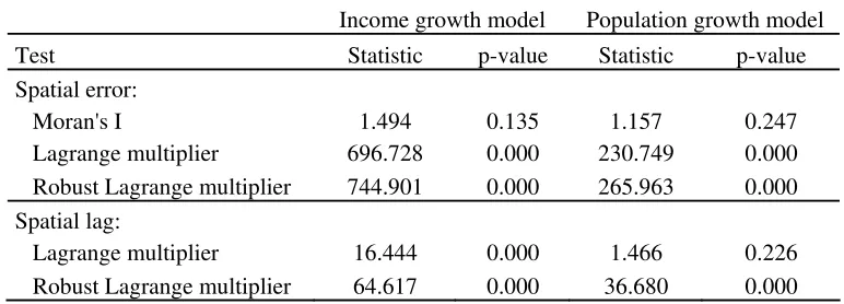
Second, we consider the extent of spatial dependence in the data and assess whether
this dependence is robust to the inclusion of the locational (geographical) fundamentals
defined in this study. To do this we apply the Lagrange multiplier and Moran’s I tests to the
residuals of the nonlinear regression analysis (3). Table 2 reports the p-values of these tests.
These p-values provide clear evidence of the statistical significance of the spatial effects for
the spatial error model, whereas for the spatial autoregressive model the statistical evidence
is mixed.
Third, we statistically assesss for the presence of threshold nonlinearities in the
above spatial models. To do this, the threshold u is estimated using the Hansen (1997)
procedure that minimises the concentrated sum of squares of the residual series indexed by
u, with u defined inside a compact set in the real line. We obtain a threshold estimate for
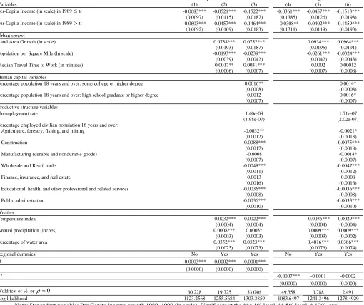
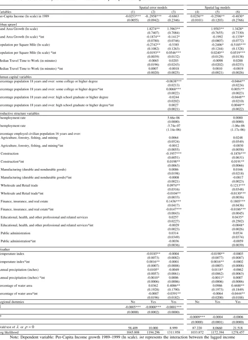
the initial per-capita income of uˆn =9.2289, which corresponds to $10,187. This threshold
estimate defines a lower regime characterised by the parameter γ11= −0.1522 for the
spatial error model and γ11 =−0.1513 for the spatial autoregressive model. Meanwhile, the
upper regime is defined by γ12 = −0.1464 for the spatial error model and γ12 =−0.1459 for
the spatial autoregressive model (see columns 3 and 6 in Table 3). These results indicate the
existence of two distinct equilibria in per-capita income growth. There are 104 cities in the
lower regime. The p-value of the nonlinearity test for the spatial versions of model (3)
given by (4) and (5) is zero, demonstrating that the differences between γ11 and γ12 are
statistically significant in both modelling strategies. Interestingly, whereas the estimates of
the regression model parameters are similar across the spatial nonlinear models, the spatial
effects are in sharp contrast. Thus, the spatial error model reports evidence of negative
serial correlation between the residuals of model (3) and provides further support to the
choice of model (4) for fitting the spatial dependence in the model errors. In contrast, the
parameter estimates of the spatial autoregressive model (5) indicate that the effect of
per-capita income between neighbouring locations vanishes when controls for geography and
social and economic factors are included.
These results are consistent with economic growth theory in that the sign of the parameters
is negative, indicating convergence towards equilibrium. Barro and Sala-i-Martin (1992),
Evans and Karras (1996), Sala-i-Martin (1996) and Evans (1997) also find statistically
significant -convergence effects using US state-level data, while Higgins et al. (2006)
use US county-level data to document statistically significant -convergence effects across
the US. Our analysis is more informative since it provides empirical evidence of the
existence of a threshold value beyond which cities achieve higher growth rates, as
0
12 11 <γ <
γ .
The second question that this article aims to answer is whether socioeconomic and
locational fundamentals can add explanatory power to the nonlinear growth model
discussed above. To assess this, we estimate both spatial models for the regression
specification without the covariates xo and without the subset of socioeconomic covariates,
namely productive structure and human capital variables (see Table 3). The results are
conclusive in showing the statistical relevance of including both sets of regressors. The
difference in log-likelihood between the models in Table 3 and the corresponding
likelihood ratio test confirm this finding. Furthermore, the signs of the coefficients are
consistent with related studies (Glaeser et al., 1995). The table also shows the statistical
significance of the spatial autoregressive model if no other covariate beyond lagged
capita income is included in the regression specification. This finding implies that
per-capita income in neighbouring locations helps explain per-per-capita income. Interestingly, the
statistical relevance of this model vanishes if the set of regressors that contain the locational
fundamentals are included in the multiple regression model. Further, the analysis of the
differences in log-likelihood between models also confirms the statistical significance of
the socioeconomic variables. These results provide mounting evidence against a strong
version of the random growth theory.
5.3. Econometric analysis of population growth
The analysis of city growth characteristics also concerns the study of population. The
supremum nonlinearity test in Hansen (1997) reports a p-value of zero and a threshold
estimate of uˆn =9.9657, which leaves 60 observations below the threshold and
corresponds to a value of 21,093 inhabitants. Recently, there has also been rising interest in
different regimes and switching points in the city size distribution literature. Ioannides and
Skouras (2013) estimate a switching point between the body of the city size distribution
and its upper tail. Using 2000 Census Places data, they show that there is a switching point
from a lognormal to a Pareto law. Curiously, the threshold level we find with our nonlinear
growth model is similar to one of the switching points estimated by Ioannides and Skouras
(2013). Their estimate for the CDGPR mixture model inspired by Combes et al. (2012) is
16,312 inhabitants with a standard deviation of 5,401.
The next step is to decide on the appropriate regression specification to test for the
existence of increasing returns to scale and to assess the importance of socioeconomic and
locational fundamentals for explaining growth in city population. Table 2 provides mixed
evidence on the relevance of using spatial models to describe the relationship between
population growth and the sets of regressors in the study. Whereas the Lagrange multiplier
test rejects the null hypothesis of no spatial effects, Moran’s I test finds no statistical
evidence to reject the null hypothesis. Based on these results, we estimate models (6) and
(7), which are robust to spatial effects.
Table 4 collects the estimates of the model parameters of the regression models (6)
error model and η11 =−0.0711 for the spatial autoregressive model. For the high growth
regime, we have η12 =−0.0691 for the spatial error model and η12 =−0.0635 for the
spatial autoregressive model (columns 3 and 6 in Table 4). These values suggest the
existence of increasing returns on population growth in US cities, because η11 <η12 <0
(see models (6) and (7)). The p-value of the corresponding nonlinearity test is zero giving
further support to the multiple equilibria hypothesis. Table 4 details the specific marginal
effects of the different variables. Our results show that the unemployment rate has no
significant effect on income growth but a very small but positive and statistically
significant influence on population growth. Unemployment’s main effect concerns
individuals’ movements rather than city’s productivity.
In contrast to the analysis of income growth, both spatial regression models are
statistically significant in all specifications for the study of population growth.
Interestingly, whereas the spatial error model reports a negative spatial correlation between
the residuals, the spatial autoregressive model indicates a positive relationship between the
population growth rates in neighbouring locations. This phenomenon suggests that
population city growth can occur because of population inflows at a regional level.
Table 1 also shows interesting insights into the differences between those cities with
low population growth rates and the national average. In contrast to the per-capita income
analysis, unemployment rates are well below the average for these cities despite slightly
lower than average educational levels. Interestingly, the structure of productive activity is
highly diversified with important contributions by the construction, manufacturing and
agriculture sectors. Location is also important; there are no cities in our sample with these
characteristics in the Northeast region of the US.
A comparison between the models in Tables 3 and 4 shows similar values for the
parameter estimates of the regressors. One exception is the parameter values of the two
human capital variables under study; increases in the percentage of population with the
highest education level (some college or higher degree) have a positive impact on
population growth, while the wider concept of human capital (high school graduate or
higher degree) has a significant negative effect. These results coincide with those of other
also find that workers have a different impact depending on their education levels (high
school or college). Finally, the study of environmental variables shows that the influence of
climate on population growth is weak, while the temperature index has a negative effect on
growth, as expected: a higher index means that the city is a harder place in which to live.
However, this coefficient loses significance in some specifications. The same applies to the
precipitation variable.
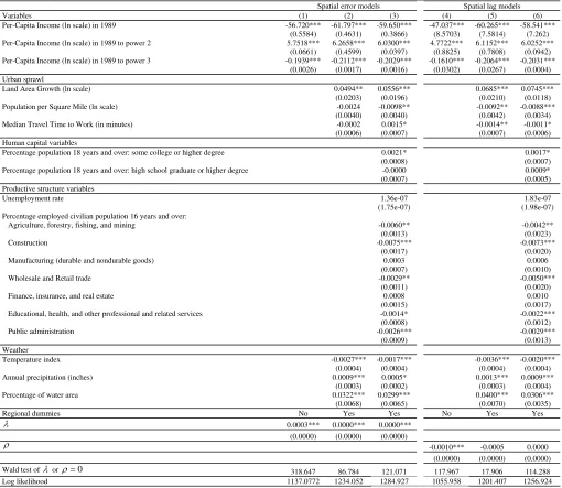
5.4. Robustness analysis
To assess the robustness of the results discussed in the preceding subsection, we carry out a
further empirical analysis. The aim of the following study is to assess the importance of the
threshold model in both of the above growth equations for determining the presence of
nonlinearities in the above convergence models. To do this we conduct three alternative
regression studies that capture potential nonlinear effects of lagged per-capita income and
population in the respective growth variables. First, we replace the threshold variables by a
polynomial of order three. This alternative modelling strategy explores the statistical
significance of higher order effects without requiring complex regression analysis. Further,
this approach is highly tractable as it relies on standard multiple linear regression analysis.
Note, however, that the method is not as explicit as the threshold model in determining the
region exhibiting the nonlinearities. Second, we consider a model the makes allowance for
interactions between the locational fundamentals and the lagged of per-capita income and
population. By doing so, the model aims to capture multiplicative effects of the variable of
interest on the response variable that are determined by the interaction of the variable with
the rest of regressors. In some cases, it seems hard to separate locational fundamentals from
increasing returns (i. e., the presence of a natural harbor or natural resources might be the
cause of local increasing returns; Ellison and Glaeser, 1999); this new specification allows
some variation of the fundamental parameters with city size. Third, we investigate the
suitability of considering threshold nonlinearities on other variables instead of on per-capita
income and lagged population.
Table 5 reports the results of the spatial tests to determine the existence of spatial
effects in the regression model considering the polynomial of order three, instead of the
threshold variables, and the regressors considering locational fundamentals. The table
model. Table 6 confirms this evidence and supports the nonlinearity of the lagged
per-capita income in explaining per-per-capita income growth. Note the lower log-likelihood values
of the models in Table 6 compared to their counterparts in Table 4. These statistics suggest
the better fit of the threshold model than of the polynomial and confirm the superior
performance of threshold models for capturing piecewise nonlinearities in the data. The
results for the polynomial model fitted to population growth are not reported because in this
example the algorithm to estimate the model parameters only shows convergence for the
simple model without locational fundamentals8. Surprisingly, the polynomial terms are not
statistically significant in the simple case. The statistics of the spatial tests reported in Table
7 provide further empirical evidence on the presence of such effects under other nonlinear
specifications of the baseline model. Table 8 reports the results for the spatial regression
models that incorporate interactions between the lagged income variable and the rest of
explanatory variables. The results suggest some relevance of the interactions between
variables, the log-likelihood function is high and comparable in some cases to the threshold
model. Interestingly, some of the locational fundamentals lose statistical significance when
combined with the rest of regressors incorporating the interactions. The results
corresponding to the analysis of population growth are surprisingly disappointing. None of
the locational fundamentals is significant in the model. The third robustness analysis
explores the suitability of alternative threshold models putting the emphasis on
nonlinearities on the locational fundamentals rather than in the endogenous income and
population variables. Unreported results provide mixed evidence on the success of such
models in explaining income and population growth. Thus, we find that human capital
variables and some productive structure variables such as manufactures, wholesale and
retail trade, and professional services exhibit nonlinearities in explaining city growth.
Nevertheless, these nonlinearities in the locational fundamentals do not change the
hypotheses tested nor the main results.
Overall, the robustness analysis confirms the existence of nonlinearities in the
relationship between lagged income and lagged population and next period’s growth. The
threshold model shows a very strong performance in terms of model fit compared to the
polynomial model and the model considering interactions with the locational fundamentals.
8
6. Conclusion
The empirical analysis of city growth has long been open to debate by researchers in urban
and geographical economics. This article has discussed three competing theories given by
increasing returns to scale leading to multiple equilibria, the importance of locational
fundamentals in determining the different equilibrium paths or the absence of any of these
theories. To assess which of these theories is better supported by the data on city growth we
have developed a cross-sectional threshold model that makes allowance in the absence of
shocks for two distinct equilibrium paths. This model incorporates a set of socio-economic
and climatological variables that proxy the locational fundamentals. We have also
considered the impact of spatial effects in city growth due to neighbouring locations and
not reflected by our set of regressors.
The conclusions of our empirical analysis that cover a sample comprising the 1,173
largest US cities confirm the existence of increasing returns to scale on both city per-capita
income and population growth in the 1990s. The threshold values that determine these
nonlinearities correspond to wealth and population levels near the left end of their
respective distributions, supporting the view that there exist some barriers to growth in
small locations. This finding is consistent with the literature on poverty traps in
macroeconomic studies of cross-sectional economic growth at the country level.
Nevertheless, our results also highlight the importance of the locational fundamentals in
explaining differences in growth across cities. These variables have in fact more
explanatory power than the threshold variables chosen to capture the endogenous growth
process. Both sets of results combined suggest that the process of city growth is
determined, to a large extent, by initial conditions. Nevertheless, there are also some other
factors that contribute to growth such as climate, the level of education or the composition
of the productive structure, amongst others.
Our results also suggest other sources of city growth not captured by the above
theories and the corresponding empirical models. Thus, we observe strong spatial effects
pointing out the significance of neighbouring effects in determining city growth. These
effects can be due to some common characteristic shared by cities in a specific region such
as climate, legislation or economic policies that make cities more or less appealing for
may be other theories, beyond and above the three aforementioned, building on the
existence of clustering effects at the county or region level that can provide alternative
explanations of city growth. Thus, these spatial effects can capture internal economies of
scale, large industry effects spilling over a region, cultural effects characteristic of a region
or state or knowledge diffusion across locations. The understanding of the variables behind
the spatial effects is beyond the scope of this paper and is left for future research.
Finally, it is worth mentioning that the period considered does not provide
conclusive evidence of one theory against the others. This is because the growth process
observed in this decade can change in former or later periods depending on several factors
(e.g. innovation cycles; see Robson, 1973; Favaro and Pumain, 2011).
Appendix 1: Data sources
The US Census Bureau offers information on a large number of variables for different
geographical levels, available on its website: www.census.gov. Using the American
FactFinder tool, you can download data from decennial census in 1990 and 2000 on most
of the variables in our study: population and per-capita income levels in 1990 and 2000,
median travel time to work, educational variables and productive structure variables. Data
on active population and unemployed people, required to construct the unemployment
rates, can also be found there. The data set containing all these economic and demographic
city variables used in the regressions is the 1990 Census Summary Tape File 3 (STF 3).
Land and water area data, needed to construct the variables land area growth, population
per square mile and percentage of water area, also come from the US Census Bureau:
http://www.census.gov/population/www/censusdata/places.html, and
http://www.census.gov/geo/www/gazetteer/places2k.html.
Finally, the source for the weather variables (temperatures used to construct the discomfort
index and annual precipitation) is the US National Oceanic and Atmospheric
Administration (NOAA), National Climatic Data Center (NCDC), Climatography of the
United States, Number 81, available online at:
References
Anselin, L. (1988). Lagrange multiplier test diagnostics for spatial dependence and spatial
heterogeneity. Geographical Analysis, 20: 1–17.
Baumol, W. (1986). Productivity Growth, Convergence, and Welfare: What the Long-Run
Data Show. American Economic Review, 76: 1072–1085.
Barro, R. J., and X. Sala-i-Martin (1992). Convergence. Journal of Political Economy,
100(2): 223–251.
Beaumont, C., C. Ertur and J. Le Gallo (2003). Spatial convergence clubs and the European
regional growth process, 1980-1995. In B. Fingleton (ed) European Regional Growth:
Springer-Verlag, 131–158.
Beeson, P.E., D. N. DeJong, and W. Troesken (2001). Population Growth in US Counties,
1840-1990. Regional Science and Urban Economics, 31: 669–699.
Berry, B. J. L. and J. D. Kasarda (1977) Contemporary Urban Ecology, New York:
Macmillan Publishing Co.
Black, D., and V. Henderson (2003). Urban evolution in the USA. Journal of Economic
Geography, 3(4): 343–372.
Bloom, D., D. Canning, and J. Sevilla (2003). Geography and Poverty traps. Journal of
Economic Growth, 8: 355–378.
Bosker, E. M., S. Brakman, H. Garretsen, and M. Schramm (2007). Looking for multiple
equilibria when geography matters: German city growth and the WWII shock. Journal of
Urban Economics, 61: 152–169.
Canova, F. (2004). Testing for convergence clubs in income per capita: a predictive density
approach. International Economic Review, 45: 49–77.
Champernowne, D. (1953). A model of income distribution. Economic Journal, LXIII:
318–351.
Chasco, C, A. López, and R. Guillain (2012). The influence of geography on the spatial
agglomeration of production in the European Union. Spatial Economic Analysis, 7(2): 247–
Combes, P.-P., G. Duranton, L. Gobillon, D. Puga, and S. Roux (2012). The Productivity
Advantages of Large Cities: Distinguishing Agglomeration from Firm Selection.
Econometrica, 80(6): 2543–2594.
Combes, P.-P., G. Duranton, and H. G. Overman (2005). Agglomeration and the
adjustment of the spatial economy. Papers in Regional Science, 84(3): 301–530.
Davis, D. R., and D. E. Weinstein (2002). Bones, Bombs, and Break Points: The
Geography of Economic Activity. The American Economic Review, 92(5): 1269–1289.
Davis, D. R., and D. E. Weinstein (2008). A search for multiple equilibria in urban
industrial structure. Journal of Regional Science, 48(1): 29–65.
De Long, J. B. (1988). Productivity Growth, Convergence, and Welfare: Comment.
American Economic Review, 78: 1138–1154.
Dobkins, L. H., and Y. M. Ioannides (2001). Spatial interactions among US cities: 1900–
1990. Regional Science and Urban Economics, 31: 701–731.
Duranton, G., and D. Puga (2001). Nursery Cities: Urban Diversity, Process Innovation,
and the Life Cycle of Products. American Economic Review 91(5), 1454-1477.
Duranton, G., and D. Puga (2004). Micro-Foundations of Urban Agglomeration
Economies. Handbook of Urban and Regional Economics, Vol. 4, J. V. Henderson and J. F.
Thisse, eds. Amsterdam: Elsevier Science, North-Holland, Chapter 48, pp. 2064–2117.
Durlauf, S., and P. Johnson (1995). Multiple Regimes and Cross-country Growth Behavior.
Journal of Applied Econometrics, 10: 365–384.
Eeckhout, J. (2004). Gibrat's Law for (All) Cities. American Economic Review, 94(5):
1429–1451.
Ellison, G., and E. L. Glaeser (1999). The geographic concentration of industry: Does
natural advantage explain agglomeration? American Economic, Review Papers and
Proceedings, 89(2): 311–316.
Evans, P. (1997). How Fast Do Economies Converge? Review of Economics and Statistics,
79(2): 219–225.
Evans, P., and G. Karras (1996). Do Economies Converge? Evidence from a Panel of U.S.
Favaro, J.-M., and D. Pumain (2011). Gibrat Revisited: An Urban Growth Model
Incorporating Spatial Interaction and Innovation Cycles. Geographical Analysis, 43: 261–
286.
Fernihough, A., and K. Hjortshøj O’Rourke, (2014). Coal and the European industrial
revolution. NBER Working Paper No. 19802.
Fingleton, B., and E. López-Bazo (2006). Empirical growth models with spatial effects.
Papers in Regional Science, 85(2): 177–198.
Gabaix, X. (1999). Zipf's law for cities: An explanation. Quarterly Journal of Economics,
114(3): 739–767.
Garmestani, A. S., C. R. Allen, and C. M. Gallagher (2008). Power laws, discontinuities
and regional city size distributions. Journal of Economic Behavior & Organization, 68:
209–216.
Glaeser, E. L., and A. Saiz (2003). The Rise of the Skilled City. Harvard Institute of
Economic Research, Discussion Paper number 2025.
Glaeser, E. L., J. A. Scheinkman, and A. Shleifer (1995). Economic growth in a
cross-section of cities. Journal of Monetary Economics, 36: 117–143.
Glaeser, E. L. and J. Shapiro (2003). Urban Growth in the 1990s: Is city living back?
Journal of Regional Science, 43(1): 139–165.
González-Val, R. (2010). The Evolution of the US City Size Distribution from a Long-run
Perspective (1900–2000). Journal of Regional Science, 50(5): 952–972.
Hansen, B. E. (1997). Inference in TAR models. Studies in Nonlinear Dynamics and
Econometrics, 2: 1–14.
Henderson, J. V. (1974). The Sizes and Types of Cities. The American Economic Review,
Vol. 64(4): 640–656.
Higgins, M. J., D. Levy, and A. T. Young (2006). Growth and Convergence Across the
U.S.: Evidence from County-Level Data. Review of Economics and Statistics, 88(4): 671–
681.
Ioannides, Y. M., and H. G. Overman (2003). Zipf’s law for cities: An empirical
Ioannides, Y. M., and S. Skouras (2013). US city size distribution: Robustly Pareto, but
only in the tail. Journal of Urban Economics, 73: 18–29.
Melo, P. C., D. J. Graham, and R. B. Noland (2009). A Meta-analysis of Estimates of
Urban Agglomeration Economies. Regional Science and Urban Economics, 39: 332–342.
Michaels, G., F. Rauch, and S. J. Redding (2012). Urbanization and Structural
Transformation. The Quarterly Journal of Economics, 127(2): 535–586.
Moran, P. A. P. (1950). Notes on Continuous Stochastic Phenomena. Biometrika, 37(1):
17–23.
Pflüger, M., and J. Südekum (2008). A synthesis of footloose-entrepreneur new economic
geography models: when is agglomeration smooth and easily reversible? Journal of
Economic Geography, Vol. 8(1): 39-54.
Plummer, P., and E. Sheppard (2006). Geography Matters: Agency, Structures and
Dynamics at the Intersection of Economics and Geography. Journal of Economic
Geography, 6(5): 619–637.
Quah, D. (1997). Empirics for Growth and Distribution: Stratification, Polarization, and
Convergence Clubs. Journal of Economic Growth, 2: 27–59.
Rappaport, J. (2007). Moving to nice weather. Regional Science and Urban Economics,
37(3): 375–398.
Roback, J. (1982). Wages, Rents, and the Quality of Life. Journal of Political Economy,
90(6): 1257–1278.
Robson, B. T. (1973). Urban growth: an approach. London: UK, Methuen.
Roos, M. W. M. (2005). How important is geography for agglomeration? Journal of
Economic Geography, Vol. 5(5): 605–620.
Rosenthal, S. S., and W. C. Strange (2004). Evidence on the Nature and Sources of
Agglomeration Economies. Handbook of Urban and Regional Economics, Vol. 4, J. V.
Henderson and J. F. Thisse, eds. Amsterdam: Elsevier Science, North-Holland, Chapter 49,
pp. 2119–2171.
Sala-i-Martin, X. (1996). Regional Cohesion: Evidence and Theories of Regional Growth
Simon, H. (1955). On a class of skew distribution functions. Biometrika, 42: 425–440.
Zheng, S., M. E. Kahn, and H. Liu (2010). Towards a system of open cities in China: Home
prices, FDI flows and air quality in 35 major cities. Regional Science and Urban
Table 1. Summary table: means and standard deviations, city variables in 1990
All sample Bottom income group Bottom population group
Variable Mean Stand. dev. Mean Stand. dev. Mean Stand. dev.
Population Growth (ln scale), 1990–2000 0.14 0.20 0.15 0.28 0.62 0.30
Per-Capita Income Growth (ln scale), 1989–1999 0.38 0.10 0.42 0.13 0.48 0.14
Urban sprawl
Land Area Growth (ln scale) 0.09 0.14 0.14 0.19 0.22 0.20
Population per Square Mile 7.90 0.77 8.03 0.91 7.05 0.73
Median Travel Time to Work (in minutes) 20.68 4.95 19.49 4.73 22.82 4.84
Human capital variables
Percent population 18 years and over: Some college or higher degree 37.85 11.76 27.09 15.08 37.02 10.41
Percent population 18 years and over: High school graduate or higher degree 58.55 9.67 45.78 14.52 56.35 9.52
Productive structure variables
Unemployment rate 6.24 2.83 10.83 4.22 4.90 3.00
Percent employed civilian population 16 years and over:
Agriculture, forestry, fishing, and mining 1.95 2.62 3.93 5.53 3.51 4.24
Construction 5.62 2.00 5.54 2.35 6.51 2.52
Manufacturing (durable and nondurable goods) 17.46 7.54 17.59 9.15 18.81 6.26
Wholesale and Retail trade 22.51 3.01 22.67 3.37 22.22 3.37
Finance, insurance, and real estate 7.08 2.62 4.56 1.39 7.08 2.53
Educational, health, and other professional and related services 24.19 6.75 24.33 9.11 20.47 4.09
Public administration 4.70 3.36 5.33 3.98 4.75 2.71
Weather
Temperature index 65.59 11.40 68.88 10.78 64.37 9.50
Annual precipitation (inches) 34.90 14.56 30.84 17.27 33.94 15.07
Percentage of water area 0.09 0.33 0.05 0.12 0.02 0.04
Regional dummy variables
Northeast Region 13.30% 8.65% 0.00%
Midwest Region 28.64% 17.31% 30.00%
South Region 27.54% 35.58% 35.00%
West Region 30.52% 38.46% 35.00%
Note: Average values of the variables under study across 1,173 observations (All sample), across the bottom per-capita income group
Table 2. Diagnostics for per-capita income and population models
Income growth model Population growth model
Test Statistic p-value Statistic p-value
Spatial error:
Moran's I 1.253 0.210 1.124 0.261
Lagrange multiplier 1039.676 0.000 252.767 0.000
Robust Lagrange multiplier 1080.431 0.000 268.014 0.000
Spatial lag:
Lagrange multiplier 1.999 0.157 8.516 0.004
Robust Lagrange multiplier 42.754 0.000 23.762 0.000
Table 3. Per-capita income growth models
Spatial error models Spatial lag models
Variables (1) (2) (3) (4) (5) (6)
Per-Capita Income (ln scale) in 1989 ≤u -0.0683*** -0.0521*** -0.1522*** -0.0361*** -0.0457*** -0.1513*** (0.0097) (0.0115) (0.0187) (0.1385) (0.0126) (0.0198) Per-Capita Income (ln scale) in 1989 >u -0.0603*** -0.0457*** -0.1464*** -0.0308** -0.0402*** -0.1459***
(0.0092) (0.0109) (0.0183) (0.1311) (0.0119) (0.0193)
Urban sprawl
Land Area Growth (ln scale) 0.0738*** 0.0752*** 0.0934*** 0.0964*** (0.0193) (0.0187) (0.0195) (0.0191) Population per Square Mile (ln scale) -0.0193*** -0.0239*** -0.0261*** -0.0324***
(0.0039) (0.0042) (0.0042) (0.0043) Median Travel Time to Work (in minutes) 0.0017** 0.0031*** 0.0002 0.00012
(0.0006) (0.0007) (0.0007) (0.0008)
Human capital variables
Percentage population 18 years and over: some college or higher degree 0.0016** 0.0014*
(0.0008) (0.0008) Percentage population 18 years and over: high school graduate or higher degree 0.0012 0.0016*
(0.0007) (0.0007) Productive structure variables
Unemployment rate 1.40e-08 1.71e-07
(1.98e-07) (2.02e-07) Percentage employed civilian population 16 years and over:
Agriculture, forestry, fishing, and mining -0.0032** -0.0021*
(0.0012) (0.0013)
Construction -0.0088*** -0.0075***
(0.0017) (0.0018) Manufacturing (durable and nondurable goods) -0.0008 -0.0014*
(0.0007) (0.0007) Wholesale and Retail trade -0.0048*** -0.0047***
(0.0011) (0.0012) Finance, insurance, and real estate 0.0013 0.0008
(0.0016) (0.0016) Educational, health, and other professional and related services -0.0036*** -0.0036***
(0.0008) (0.0008) Public administration -0.0036*** -0.0033***
(0.0010) (0.0010)
Weather
Temperature index -0.0032*** -0.0022*** -0.0036*** -0.0029*** (0.0004) (0.0004) (0.0004) (0.0004) Annual precipitation (inches) 0.0008*** 0.0005* 0.0009*** 0.0009***
(0.0003) (0.0003) (0.0003) (0.0002) Percentage of water area 0.0352*** 0.0323*** 0.4016*** 0.0386***
(0.0075) (0.0073) (0.0076) (0.0074)
Regional dummies No Yes Yes No Yes Yes
λ -0.0003*** -0.0002*** -0.0001***
(0.0000) (0.0000) (0.0000)
ρ -0.0007*** -0.0001 -0.0002
(0.0000) (0.0000) (0.0000) Wald test of λ or ρ=0 60.228 19.725 33.046 49.358 0.788 2.491 Log likelihood 1123.2568 1255.5684 1303.3859 1083.6497 1241.3496 1278.4929