Remote Sensing Letters
Vol. 00, No. 00, 00 Month 201X, 1–10
RESEARCH ARTICLE
Comparison of Approximation Methods to Kullback-Leibler Divergence between Gaussian Mixture Models for Satellite Image
Retrieval Shiyong Cui
Remote Sensing Technology Institute (IMF), German Aerospace Center (DLR), Oberpfaffenhofen, 82234 Wessling, Germany
(April 6, 2016)
As a probabilistic distance between two probability density functions, Kullback-Leibler divergence is widely used in many applications, such as image retrieval and change detection. Unfortunately, for some models, e.g., Gaussian Mixture Models (GMMs), Kullback-Leibler divergence is not analytically tractable. One has to resort to approx-imation methods. A number of methods have been proposed to address this issue. In this letter, we compare seven methods, namely Monte Carlo method, matched bound approximation, product of Gaussians, variational method, unscented transformation, Gaussian approximation, and min-Gaussian approximation, for approximating the Kullback-Leibler divergence between two Gaussian mixture models for satellite im-age retrieval. Two experiments using two public datasets have been performed. The comparison is carried out in terms of retrieval accuracy and computational time.
Keywords:Gaussian Mixture Models (GMMs), Kullback-Leibler Divergence, Image retrieval.
1. Introduction
As a probabilistic distance between two probability density functions, Kullback-Leibler divergence (Kullback and Kullback-Leibler 1951) is widely used for comparing two statistical models in many applications, such as multi-temporal image analysis and image retrieval. In (Heas and Datcu 2005), the Kullback-Leibler divergence was used to compare two time-localized distributions in order to model the trajectories of dynamic clusters in image time-series. It was applied to change detection in (Inglada and Mercier 2007) by analyzing the the evolution of the local statistics of the image between two dates. The degree of evolution of the local statistics is measured using the Kullback-Leibler divergence. It was applied also in the wavelet domain (Cui and Datcu 2012) to detect changes in synthetic aperture radar images. In image retrieval, the most common approach is to compare two images using a similarity measure based on a representation of the image content by a feature space. A large amount of work can be found from the literature, such as the earth mover’s distance (Rubner et al. 2000), the fast compression distance (Cerra and Datcu 2012), the Kullback-Leibler divergence (Choy and Tong 2010), to name a
few. Among them, the Kullback-Leibler divergence is one of the most popular similarity measures for comparing images. For instance, in (Choy and Tong 2010), the Kullback-Leibler divergence was used to assess the similarity of two images by comparing the distributions of wavelet coefficients. In (Piro et al. 2008), it was applied in thek-nearest neighbors (k-NN) framework to image retrieval based on sparse multiscale image representations. A texture-image retrieval approach was proposed in (Kwitt and Uhl 2008) by measuring the Kullback-Leibler divergence between the marginal distributions of complex wavelet coefficient magnitudes. A novel wavelet-based texture retrieval method was developed in (Do and Vetterli 2002) by using a closed-form Kullback-Leibler distance between the generalized Gaussian density distributions.
However, for some parametric models in retrieval, the integral involved in com-puting the Kullback-Leibler divergence is not analytically tractable, which is the case for Gaussian mixture models (GMMs). Nevertheless, GMM is a popular sta-tistical model due to its flexibility. Therefore, one has to resort to approximations to the Kullback-Leibler divergence between two GMMs. In literature, a number of methods have been proposed for approximation. However their performances on approximation are not well understood. Thus, in this letter, we compare seven methods for approximating the Kullback-Leibler divergence between two GMMs in satellite image retrieval. We first extract some local features from an image and then estimate a parametric GMM for the feature space. The learned model is considered as a statistical representation of the image content. Then the Kull-backLeibler divergence between GMMs is approximated by these methods. Two experiments using two public datasets have been performed. The comparison is carried out in terms of retrieval accuracy and computational time.
In the following sections, an image is represented by a random variableX taking valuesxfrom addimensional spaceRd. The low-level features extracted from the images are denoted byxn andpX(x) denotes the model of imageX.Ni(X;µi,Σi) is a multivariate Gaussian distribution with a mean vector µi and a covariance matrixΣi
2. Kullback-Leibler Divergence Approximation Methods
Given a query imageX and a database of images Yq, q= 1,· · ·, Q, the goal is to retrieve a set of images with similar content as the query. To this end, we perform three steps. The first step is to extract low-level features {x1,x2,· · · ,xN} from both the query and all images in the database. The second step is to learn a GMM model pX(x) as a representation of the image content using the low-level features xn extracted from an image. The final step is to evaluate the Kullback-Leibler divergence between the modelpX(x) of the query image X and the model
pYq(x) of each image Yq in the database. In the following description, we drop the subindex ofY for the sake of notational brevity. In the next two sections, we present a method to estimate a GMM model and approximation methods to the Kullback-Leibler divergence between two GMMs.
2.1 Gaussian Mixture Model
A random variableXfollows a Gaussian mixture distribution if its probability den-sity function can be written aspX(x) =PMi=1βiNi(X;µi,Σi), whereβiis the prior probability of each component. To apply this model to a feature space of an image,
one has to estimate the governing parameters Θ ={β1,µ1,Σ1,· · · , βM,µM,ΣM} using a set of low-level features {x1,x2,· · · ,xN} as training data. The standard method to estimate the parameters of a GMM is the Expectation-Maximization (EM) algorithm (Dempster et al. 1977). However, one needs to choose an appropri-ate number of Gaussian components. A number of model selection methods, such as Bayesian Information Criterion (BIC) (Schwarz 1978) and Akaike Information Criterion (AIC) (Akaike 1973), are available in the literature. In this letter, BIC defined by (1) is used for choosing the number of Gaussian components.
BIC(Θ) =−2 lnL(Θ|X) +Klnd (1)
L(Θ|X) is the likelihood function, K is the number of parameters, and d is the dimensionality of the low-level feature vector. If there is only one Gaussian com-ponent in each GMM, the Kullback-Leibler divergenceD(X||Y) defined in (2)
D(X||Y) = Z pX(x) ln pX(x) pY(x) dx (2)
turns down to that between two Gaussian distributions pX(x) = N(X;µX,ΣX) andpY(x) =N(Y;µY,ΣY). In this case, we have an analytical formula in (3).
D(X||Y) = 1 2{tr Σ −1 Y ΣX + (µY −µX)TΣ−Y1(µY −µX)−d−ln|ΣX| |ΣY| } (3)
In (3), T and tr denote the transpose and the trace of a matrix, Unfortunately, if there are more than one Gaussian component in two GMMs, the Kullback-Leibler divergence is not analytically tractable. Thus, we have to resort to approximation methods.
2.2 Approximation Methods
Given two GMMs pX(x) = PMi=1βiNi(X;µi,Σi) and pY(x) = PN
j=1αjNj(Y;µ0j,Σ
0
j), our goal is to compute the Kullback-Leibler diver-gence between them. In the following description, for the brevity of notations, we denote the Gaussian components of pX(x) and pY(x) by piX(x) = Ni(X;µi,Σi) andpjY(x) =Nj(Y;µ0j,Σ
0
j). 2.2.1 Monte Carlo Sampling
The fundamental idea is to draw a large number of samples {xk}Sk=1 frompX(x) and use these samples to replace the integral by a summation over all samples. Thus, the Kullback-Leibler divergence,DMC(X||Y), can be approximated as
DMC(X||Y) = 1 S S X i=1 lnpX(xi)−lnpY(xi) (4)
If the number of samples S used for approximation goes to infinite, the approx-imation will be very close to the true value of the Kullback-Leibler divergence. Practically, we need to draw a large number of samples {xk}Sk=1 from a GMM. We first select a Gaussian component according to their prior probabilities βi. Then we draw a sample xk from the selected Gaussian component Ni(X;µi,Σi).
This procedure is repeated many times in order to obtain an accurate approxima-tion. The Monte Carlo method is the only method that can really estimate the Kullback-Leibler divergence provided a large number of independent and identi-cally distributed samples are available.
2.2.2 Gaussian Approximation
This method first approximatespX(x) andpY(x) by two Gaussian distributions ˆ
pX(x) = N(X;µX,ΣX) and ˆpY(x) = N(Y;µY,ΣY). The mean and covariance matrix can be estimated by those of each component as follows
µX = M X i=1 βiµi, ΣX = M X i=1 βi(Σi+ (µi−µX)(µi−µX)T). (5)
Similarly, µY and ΣY can also be estimated as well. Then the Kullback-Leibler divergence between pX(x) and pY(x) can be approximated by that of these two Gaussian distributions ˆpX(x) and ˆpY(x) based on (3). Another popular choice of Gaussian approximation is to use the minimum Kullback-Leibler divergence,
Dmin(X||Y), between their Gaussian components, as shown in (6). Dmin(X||Y) = min i,j D(Ni(X;µi,Σi)||Nj(Y;µ 0 j,Σ 0 j)) (6) Although it is simple to formulate, but the identification property (Hershey and Olsen 2007) does not hold and it is prone to underestimateD(X||Y).
2.2.3 The Product of Gaussian Approximation
This method is derived based on an upper bound of the likelihood resulted from Jensen’s inequality (Hershey and Olsen 2007). Since likelihood and Kullback-leibler divergence have the following relation
D(X||Y) =EpX(x)[lnpX(x)]−EpX(x)[lnpY(x)], (7) whereE[·] denotes the expectation, the Kullback-Leibler divergence can be approx-imated by an estimate of the likelihood. Based on Jensen’s inequality f(E[x]) ≤
E[f(x)], an upper bound of the likelihood can be derived as (8),
EpX(x)[lnpY(x)] = M X i=1 βiEpi X(x) h ln N X j=1 αjpjY(x) i ≤ M X i=1 βiln N X j=1 αjEpi X(x)[p j Y(x)] = M X i=1 βiln N X j=1 αjCij. (8) Cij = R
piX(x)pjY(x)dx is the normalization constant of a product of two Gaus-sian distributions. Therefore, the Kullback-Leibler divergence,DPoG(X||Y), can be
approximated using the above upper bound, as shown in (9).
DPoG(X||Y) = M X i=1 βiln PM k=1βkCik PN j=1αjCij Cik= Z piX(x)pkX(x)dx (9)
2.2.4 The Unscented Transformation
The unscented transformation (Julier and Uhlmann 1997a; Goldberger et al. 2003) is a method to estimate the expectationEf(x)[h(x)] of a functionh(x) with
respect to a Gaussian probability density functionf(x) =N(X;µ,Σ). It has been successfully applied in nonlinear filtering (Julier and Uhlmann 1997b). Following the same idea as Monte Carlo approximation, the expectation can be estimated by a set of samples xi drawn from f(x). In contrast, this method deterministically selects only 2d “sigma” points {xk}2kd=1 with weights 1/2d from the distribution
f(x) for estimation. Thus, the expectation can be estimated as
Ef(x)[h(x)] = 1 2d 2d X k=1 h(xk). (10)
One popular choice of the sigma points for a Gaussian distributionNi(X;µi,Σi) is as follows:
xi,k =µi+
p
dλi,kei,k, xi,d+k=µi− p
dλi,kei,k, k= 1, ..., d, (11) whereλi,kandei,kare the eigenvalues and eigenvectors of the covariance matrixΣi. Therefore, 2d “sigma” points xi,k, k = 1, ...,2d can be drawn from each Gaussian component ofpX(x) and are used to approximate the Kullback-Leibler divergence,
Dustd(X||Y), as follows: Dustd(X||Y) = 1 2d M X i=1 βi 2d X k=1 lnpX(xi,k) pY(xi,k) (12)
2.2.5 The Matched Bound Approximation
The matched bound approximation (Goldberger et al. 2003) approximates the Kullback-Leibler divergence by minimizing a matching function that finds the clos-est weighted Gaussian componentm(i) ofpY(x) to that ofpX(x). It has two steps. The first step is to find the closest weighted Gaussian component ofpY(x) to each component of pX(x). Formally, we solve the minimization problem (13) for each
piX(x). m(i) = argmin j D(p i X(x)||p j Y(x))−lnαj (13) Then we use the matched pairs (m(i), i) of Gaussian components to approximate the Kullback-Leibler divergence byDM BA(X||Y) as follows
DMBA(X||Y) = M X i=1 βi D(piX(x)||pYm(i)(x)) + ln βi αm(i) . (14)
2.2.6 The Variational Approximation
Variational approximation (Hershey and Olsen 2007) is based on a variational lower bound of the likelihood EpX(x)[lnpY(x)] obtained by introducing a set of variational parametersφj|i >0,
P
a lower bound in (15). EpX(x)[lnpY(x)] =EpX(x) h ln N X j=1 αjpjY(x) i =EpX(x)hln N X j=1 φj|i αjpjY(x) φj|i i ≥EpX(x) N X j=1 φj|iln αjpjY(x) φj|i = M X i=1 N X j=1 βiφj|i ln αj φj|i +Epi X(x)[lnp j Y(x)] . (15) We then maximize this lower bound and solve forφj|i, which is given by (16).
ˆ φj|i = αjexp −D(pi X(x)||p j Y(x)) PN j=1αjexp −D(pi X(x)||p j Y(x)) (16)
Then the lower bound can be computed by substituting (16) into (15). Likewise, we can derive a lower bound of EpX(x)[lnpX(x)]. Finally, the Kullback-Leibler di-vergence between pX(x) and pY(x) can be approximated by Dv(X||Y) given in
(17). Dv(X||Y) = M X i=1 βiln M X j=1 βjexp −D(piX(x)||pjY(x)) N X j=1 αjexp −D(piX(x)||pjY(x)) (17)
3. Experiments and Discussions
In this section, we present the datasets used for comparison and the results of our experiments.
3.1 Datasets
3.1.1 UCMerced Land Use Dataset
The first dataset is the UCMerced land use dataset (Yang and Newsam 2010), which is available at http://vision.ucmerced.edu/datasets/landuse.html. The images were manually extracted from large images existing in the USGS na-tional map urban area imagery collection covering various urban areas around US. The image has pixels of 0.3 m. The dataset comprises 21 classes, namely agri-cultural, airplane, baseball diamond, beach, buildings, chaparral, dense residential, forest, freeway, golf course, harbor, intersection, medium residential, mobile home park, overpass, parking lot, river, runway, sparse residential, storage tanks, tennis court. Each class has 100 images with a size of 256×256 pixels. Example images from each class are shown in Figure 1.
3.1.2 Wuhan High-resolution Satellite Scene Dataset
The Wuhan dataset, available at http://dsp.whu.edu.cn/cn/staff/yw/ HRSscene.html, contains 18 classes of images, including airport, bridge, desert,
Figure 1. Example images of the UCMerced dataset.
farmland, football field, forest, meadow, mountain, park, parking, pond, port, rail-way station, river, viaduct, commercial area, industrial area, and residential area . In each class, there are 50 samples with a size of 600×600 pixels. Each class is collected from different regions in satellite images of different resolutions and they might have different scales, orientations and illuminations. Example images from each class are shown in Figure 2.
Figure 2. Example images of the Wuhan dataset.
3.2 Results and Discussions
We use each image as a query and search for similar images among the remaining images. We first learn GMM models using the RGB pixel values based on the algorithm presented in section 2.1, which can automatically estimate the number of Gaussian components. Then we use the estimated parameters and the seven methods for approximating the Kullback-Leibler divergence between two GMMs. Due to its asymmetrical property, the symmetrical version is used. For evaluation, we use the precision-recall curve. As an overall accuracy measure, the area under this curve (AUC) is also computed and compared. Since the precision-recall curve has a distinctive saw-tooth shape, the average interpolated precision-recall cures (Manning et al. 2008) over all queries are used for comparison. In addition, we also compare the computing time. For the method of Monte Carlo sampling, we use a sample of 80,000 points for approximation.
Table 1. Average AUC (%) and CPU time of the seven methods for the UCMerced dataset. The best one is marked by bold font. The seven methods, namely Monte Carlo method, matched bound approximation, product of Gaussians, variational method, unscented transformation, Gaussian approximation, and min-Gaussian approximation, are indexed from 1 to 7 in this table.
Methods 1 2 3 4 5 6 7.
Average AUC (%) 21.51 21.58 19.87 21.82 21.43 20.89 16.33 CPU time (s) 0.2157 0.0100 0.0150 0.0358 0.0297 0.0014 0.0265
0.0 0.1 0.2 0.3 0.4 0.5 0.6 0.7 0.8 0.9 1.0 0.0 0.1 0.2 0.3 0.4 0.5 0.6 0.7 0.8 0.9 1.0 Recall Average Precision (%)
Variational Approximation, AUC = 0.21823 Matched Bound Approximation, AUC = 0.21578 Monte Carlo, AUC = 0.21511
Unscented Transformation, AUC = 0.21434 Gaussian Approximation, AUC = 0.2089 Product of Gaussians, AUC = 0.19866 min−Gaussian Approximation, AUC = 0.16326
(a) 0.0 0.1 0.2 0.3 0.4 0.5 0.6 0.7 0.8 0.9 1.0 0.0 0.1 0.2 0.3 0.4 0.5 0.6 0.7 0.8 Recall Average precision (%)
Gaussian Approximation, AUC = 0.28091 Variational Approximation, AUC = 0.28001 Matched Bound Approximation, AUC = 0.27652 Unscented Transformation, AUC = 0.27378 Monte Carlo, AUC = 0.2736
Product of Gaussians, AUC = 0.26509 min−Gaussian Approximation, AUC = 0.21442
(b) 0.0 0.1 0.2 0.3 0.4 0.5 0.6 0.7 0.8 0.9 1.0 0.0 0.1 0.2 0.3 0.4 0.5 0.6 0.7 0.8 0.9 1.0 Recall Average precision (%)
Gaussian Approximation, AUC = 0.26872 Variational Approximation, AUC = 0.24046 Matched Bound Approximation, AUC = 0.24601 Unscented Transformation, AUC = 0.22826 Monte Carlo, AUC = 0.2303
Product of Gaussians, AUC = 0.17559 min−Gaussian Approximation, AUC = 0.18382
(c)
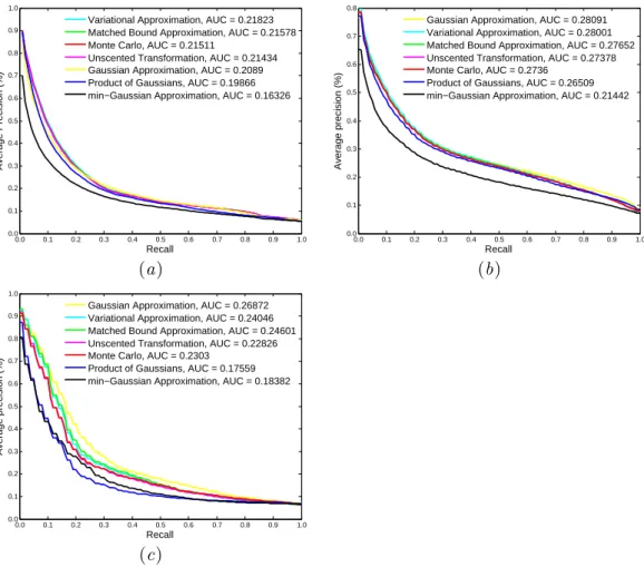
Figure 3. Experimental results: (a) average precision-recall curves and AUCs of the seven approximation methods on the UCMerced dataset; (b) average precision-recall curves and AUCs of the seven approxima-tion methods on the Wuhan dataset; (c) average precision-recall curves and AUCs of the seven methods for the classmeadow.
UCMerced dataset are shown in Figure 3(a). The average CPU time are shown in Table 1. From the results, we can observe that the variational approximation performs best with an average AUC of 0.2182. The matched bound approximation ranks second but with much less computing time than the variational method. In addition, although we used a large sample of 80,000 points in the Monte Carlo sampling, it is still not enough if we compare it with the variational approximation. Furthermore, compared with other methods, the Monte Carlo method is compu-tationally very slow, which limits its use in some applications such as change de-tection because the computation has to be performed at all pixels. min-Gaussian is the most inferior method and the Gaussian approximation is the fastest one. Additionally, we can also observe that the matched bound approximation and the unscented transformation have similar performances that are only slightly lower than the variational approximation method. The method of product of Gaussians performs even inferiorly than the Gaussian approximation.
Table 2. Average AUC (%) and CPU time of the seven methods for the Wuhan dataset. The best one is marked by bold font. The seven methods, namely Monte Carlo method, matched bound approximation, product of Gaussians, variational method, unscented transformation, Gaussian approximation, and min-Gaussian approximation, are indexed from 1 to 7 in this table.
Methods 1 2 3 4 5 6 7.
Average AUC (%) 27.36 27.65 26.51 28.00 27.38 28.09 21.44 CPU time (s) 0.4439 0.0303 0.0468 0.0447 0.0330 0.0020 0.0217
The results of the experiments using the second dataset (Wuhan dataset) is presented in Figure 3(b). Similarly as the previous experiment, min-Gaussian per-forms least among the seven methods. Nevertheless, the Gaussian approximation performs best with an average AUC of 0.2687 and has the lowest computational complexity of 0.0020s. The main reason is that, for some homogeneous classes. e.g., forest, meadow, desert, the assumed GMM distribution boils down to a Gaussian distribution. For example, the average precision-recall curves of the seven meth-ods for class meadow are shown in Figure 3(c). The variational method performs only slightly worse than the Gaussian approximation. As in the first experiment, we can also observe that the matched bound approximation and the unscented transformation have similar performances that are only slightly inferior than the variational approximation method. But they can be computed faster than the vari-ational method. The method of product of Gaussians performs similarly as that in the first experiment.
4. Conclusion
In this letter, we compare seven methods, namely Monte Carlo method, matched bound approximation, product of Gaussians, variational method, unscented trans-formation, Gaussian approximation, and min-Gaussian approximation, for approx-imating the Kullback-Leibler divergence between two Gaussian mixture models for satellite image retrieval. Two experiments using two public datasets have been performed. In principle, Monte Carlo method can achieve high accuracy provided a large number of samples are available. Nevertheless, as shown in the evalua-tion, it has a similar performance as the unscented transformation. Practically, Monte Carlo method is not applicable due to its high computational complexity. Variational approximation seems a good compromise between computation and accuracy. If the images are homogeneous, Gaussian approximation will be a good choice which is the case in the second evaluation. The matched bound approxima-tion and the unscented transformaapproxima-tion perform slightly worse than the variaapproxima-tional method. min-Gaussian is generally not a good choice.
References
Akaike, H. (1973). Information theory and an extension of the maximum likelihood prin-ciple. In B. N. Petrov and F. Csaki (Eds.),Second International Symposium on Infor-mation Theory, Budapest, pp. 267–281. Akademiai Kiado.
Cerra, D. and M. Datcu (2012, Feb.). A Fast Compression-based Similarity Measure with Applications to Content-based Image Retrieval. Journal of Visual Communication and Image Representation 23(10), 293–302.
Choy, S. K. and C. S. Tong (2010, Feb.). Statistical Wavelet Subband Characterization Based on Generalized Gamma Density and Its Application in Texture Retrieval. IEEE Transactions on Image Processing 19(2), 281–289.
Cui, S. and M. Datcu (2012, Aug.). Statistical Wavelet Subband Modeling for Multi-Temporal SAR Change Detection. IEEE Journal of Selected Topics in Applied Earth Observations and Remote Sensing 5(4), 1095–1109.
Dempster, A., N. Laird, and D. Rubin (1977). Maximum likelihood from incomplete data via the EM algorithm. Journal of the Royal Statistical Society, Series B 39(1), 1–38. Do, M. N. and M. Vetterli (2002, Feb.). Wavelet-based texture retrieval using generalized
Gaussian density and Kullback-Leibler distance. IEEE Transactions on Image Process-ing 11(2), 146–158.
Goldberger, J., S. Gordon, and H. Greenspan (2003). An efficient image similarity measure based on approximations of KL-divergence between two gaussian mixtures. InComputer Vision, 2003. Proceedings. Ninth IEEE International Conference on.
Heas, P. and M. Datcu (2005, Jul.). Modeling Trajectory of Dynamic Clusters in Image Time-Series for Spatio-Temporal Reasoning. IEEE Trans. Geosci. Remote Sens. 43(7), 1635–1647.
Hershey, J. R. and P. A. Olsen (2007, Apr.). Approximating the Kullback Leibler Diver-gence Between Gaussian Mixture Models. InAcoustics, Speech and Signal Processing, 2007. ICASSP 2007. IEEE International Conference on, Volume 4, pp. IV–317–IV–320. Inglada, J. and G. Mercier (2007, May). A new statistical similarity measure for change detection in multitemporal sar images and its extension to multiscale change analysis. IEEE Transactions on Geoscience and Remote Sensing. 45(5), 1432–1445.
Julier, S. J. and J. K. Uhlmann (1997a). A Consistent, Debiased Method for Converting Between Polar and Cartesian Coordinate Systems. InIn The Proceedings of AeroSense: The 11th International Symposium on Aerospace/Defense Sensing, Simulation and Con-trols, pp. 110–121.
Julier, S. J. and J. K. Uhlmann (1997b). A new extension of the Kalman filter to nonlinear systems. In Proc. of AeroSense: The 11th Int. Symp. on Aerospace/Defence Sensing, Simulation and Controls.
Kullback, S. and R. A. Leibler (1951). On information and sufficiency. Annals of Mathe-matical Statistics 22, 49–86.
Kwitt, R. and A. Uhl (2008, Oct.). Image similarity measurement by Kullback-Leibler divergences between complex wavelet subband statistics for texture retrieval. InImage Processing, 2008. ICIP 2008. 15th IEEE International Conference on, pp. 933–936. Manning, C. D., P. Raghavan, and H. Sch¨utze (2008). Introduction to Information
Re-trieval. New York, NY, USA: Cambridge University Press.
Piro, P., S. Anthoine, E. Debreuve, and M. Barlaud (2008, June). Image retrieval via Kullback-Leibler divergence of patches of multiscale coefficients in the KNN framework. InInternational Workshop on Content-Based Multimedia Indexing (CBMI), 2008, pp. 230–235.
Rubner, Y., C. Tomasi, and L. J. Guibas (2000, Nov.). The Earth Mover’s Distance As a Metric for Image Retrieval. International Journal of Computer Vision 40(2), 99–121. Schwarz, G. (1978). Estimating the Dimension of a Model. The Annals of Statistics 6(2),
461–464.
Yang, Y. and S. Newsam (2010). Bag-Of-Visual-Words and Spatial Extensions for Land-Use Classification. In Proc. 18th SIGSPATIAL International Conference on Advances in Geographic Information Systems, GIS ’10, New York, NY, pp. 270–279.