Large-Eddy Simulation of Axisymmetric Compression Corner Flow

Large-Eddy Simulation of Axisymmetric

Compression Corner Flow

Prahladh S. Iyer∗

National Institute of Aerospace, Hampton, VA 23666 Mujeeb R. Malik†

NASA Langley Research Center, Hampton, VA 23681

The Wall-Modeled Large Eddy Simulation (WMLES) approach is used to study the inter-action of a shock wave with a high Reynolds number turbulent boundary layer. Since the near wall region is modeled, high Reynolds number turbulent flows can be simulated at a moder-ate computational cost. The case considered is that of an axisymmetric Mach 2.85 turbulent boundary layer over a 30◦compression corner. The Reynolds number of the boundary layer upstream of the interaction based on momentum thickness (Reθ =u∞θ/ν∞) is≈12,000. The geometry and flow conditions match the experiments of Dunagan et al. (NASA TM 88227, 1986). The simulations were performed using equilibrium and non-equilibrium wall models. The agreement with experiment is encouraging for the finest grid with respect to the separation bubble length, unsteady shock structure and wall pressure distribution. Sensitivity of WMLES results to grid, wall model, and blockage effects in the tunnel are reported.

I. Introduction

High fidelity simulation methodologies are required to improve our understanding of flows over complex geometries. Computational Fluid Dynamics (CFD) can play a critical role in the design of high-speed vehicles since ground-based testing is expensive. Reynolds-averaged Navier-Stokes (RANS)-based methods are currently widely used for high Reynolds number turbulent flows but are not accurate for complex flows involving separation. High fidelity Direct Numerical Simulation (DNS) and Large Eddy Simulation (LES) methods, while accurate, are infeasible for realistic flight Reynolds number flows. Hence, hybrid RANS/ LES methods such as Wall-modeled LES (WMLES) are becoming increasingly popular for such high Reynolds number flows in complex geometries.

The recent reviews by Larsson et al. [1] and Bose & Park [2] discuss the various aspects related to the application of wall-modeled LES to complex turbulent flows. Wall-modeled LES can be further classified into wall-stress models and hybrid RANS/ LES methods. Wall-stress models apply a stress boundary condition, typically obtained by solving RANS-like wall-model equations. Cabot & Moin [3] and Piomelli & Balaras [4] discuss various wall models commonly used in WMLES simulations. More recent wall models include those by Kawai & Larsson [5, 6], Park & Moin [7], Bose & Moin [8] and Yang et al. [9]. While most wall stress models work well for canonical attached flows such as channel and flat plate boundary layers, their ability to accurately predict turbulent separated flows is an area of ongoing research. Detached-Eddy Simulation (DES), and its variants such as Delayed DES (DDES) and Improved Delayed DES (IDDES), is another popular hybrid RANS/ LES technique applied to highReturbulent flows (see Spalart [10]).

IDDES, when run in WMLES mode, resolves the flow away from the wall and models the near wall region. This has been successfully applied to a number of turbulent separated flows by Shur et al. [11].

The interaction of a shock wave with turbulent boundary layer is complex and challenging to predict, owing to the combined effects of shocks, turbulence and separation. While various experiments have been performed to understand this interaction, eddy resolving simulations (DNS/ LES) have largely been limited to lower Reynolds number flows. An experimental database of shock/ turbulence interactions with data from various experiments can be found in Settles & Dodson [12]. Review papers regarding shock/ turbulence interaction can be found in Andreopoulos et al. [13], Knight et al. [14] and Gaitonde [15]. Experiments for a compression corner interaction have been performed by various researchers such as Settles et al. [16], Dolling & Murphy [17] and Smits & Kin-Choon [18]. DNS/ LES of compression corner shock/ boundary layer interactions have been performed by Adams [19], Rizzetta et al. [20], Loginov et al. [21] and Wu & Martin [22], among others.

∗_{Research Scientist, AIAA Member.}

†_{Senior Aerodynamicist, Computational AeroSciences Branch, MS 128, AIAA Fellow.}

We simulate the experimental conditions of Dunagan et al. [23] and Brown et al. [24] where a Mach 2.85 turbulent boundary layer with a unit Reynolds number of 18 million/m is incident on a 30◦_{compression corner. Detailed velocity,} density and turbulent stress data are available in the interaction region for comparison. A recent study by DeBonis [25] for the same flow configuration using Reynolds-Averaged Navier-Stokes (RANS) methodology found that among four popular industry standard models, only the Spalart-Allmaras model produced reasonable predictions, with further scope for improvement. We assess the performance of the WMLES approach for this problem by making detailed comparisons with available experimental data. The same approach was previously used by Bermejo-Moreno et al. [26] to study oblique shock/ turbulence interaction and obtained good agreement with experiment. Also, we have previously used this approach to study turbulent separated flows at subsonic [27] and transonic [28] conditions.

The paper is organized as follows. The details of the flow solver and wall model are briefly discussed in Section II. The flow conditions and computational grid details are discussed in Section III; and results, including qualitative and quantitative comparison to experiment, are presented in Section IV. Sensitivity of the results to various parameters such as grid, wall model and spanwise domain width are discussed in Section IV.C. A brief summary in Section V concludes the paper.

II. Numerical Details

The Charles solver∗_{is used in the simulations. This code solves the compressible Navier-Stokes equations on} unstructured grids by using a cell-centered finite-volume methodology. The solver is second-order accurate in space for unstructured grids. An explicit third-order Runge-Kutta scheme is used for time advancement. The constant coefficient Vreman model was used to model the subgrid terms. The solver uses an ENO-based reconstruction scheme with an HLLC flux for shock capturing. Further details about the numerics can be found in Khaligi et al. [29]. The solver has been applied to a wide range of problems such as shock/ turbulence interaction (Bermejo-Moreno et al. [26]) and supersonic jets (Bres et al. [30]).

Two wall models are used in this study: (i) equilibrium wall model of Kawai and Larsson [5], and (ii) non-equilibrium wall model of Park and Moin [7]. The equilibrium wall model solves a system of coupled ordinary differential equations (ODE) by applying the boundary-layer approximation, and retaining only the wall-normal terms in the compressible Navier-Stokes equations. While this is valid for attached regions of the flow, it does not capture non-equilibrium effects in accelerating and separated regions of the flow. Hence, the accuracy of the prediction in non-equilibrium regions is dependent on how much these effects are captured by the outer layer (resolved by LES) and the grid resolution in the region. The non-equilibrium wall model uses the full compressible Navier-Stokes equations without neglecting any terms. Both wall models use a mixing-length based turbulent eddy viscosity in the wall model equations. The Park and Moin [7] model uses a dynamic correction of the Karman constant in the mixing-length model to account for the portion of turbulent stresses resolved due to the unsteady boundary conditions from LES. We have previously used these wall models to study separated flows past a wall-mounted hump [27] and axisymmetric transonic bump [28].

Complimentary Reynolds-Averaged Navier-Stokes (RANS) simulations were carried out using the FUN3D solver [31], with the Spalart-Allmaras (SA) model, since the results of DeBonis [25] indicated that the SA model overall best predicted this flow among other popular RANS models. The grid and boundary conditions were identical to the simulations of DeBonis. The only difference was that the flow Reynolds number was taken to be 18 million/m instead of the value of 16 million/m (corresponding to the experiments of Brown et al. [24]) used by DeBonis [25]. The effect of Reynolds number was small with a difference of≈4% (w.r.t. experimental value) in the separation bubble length.

III. Problem Description

The interaction of a high Reynolds number supersonic turbulent boundary layer at Mach 2.85 with an axisymmetric 30◦_{compression corner is studied at conditions matching the experiments of Dunagan et al. [23]. This configuration} is a test case for the NASA Revolutionary Computational Aerosciences (RCA) challenge under the Transformational Tools and Technologies (TTT) project, and is a challenging flow to predict owing to the complex interaction of shocks, turbulence and flow separation. A schematic of the interaction under study is shown in Figure 1, which is taken from Sfeir [32]. As the turbulent boundary layer approaches the compression corner, it separates due to the adverse pressure gradient giving rise to a separation bubble whose length is typically of the order of the boundary layer thickness of the upstream flow. Since the flow is supersonic, a shock is formed due to the deflection of the flow streamlines in the vicinity of separation and reattachment, both of which are depicted in the figure. Depending on the conditions, the

shocks may coalesce to form a single shock.

S∗ R∗

Fig. 1 A schematic of the shock/ boundary layer interaction in a compression corner is reproduced from Sfeir [32] to indicate the main flow features. The boundary layer separates (S) upstream of the compression corner due to adverse pressure gradient and reattaches (R) downstream of the corner. The shock formed due to separation (S∗) and reattachment (R∗) are depicted in the figure.

The experimental setup of Dunagan et al. [23] is reproduced in Figure 2. While the compression corner model is axisymmetric, it is important to note that deviations from axisymmetry of the shock/ turbulence interaction are possible due to rectangular shape of the wind tunnel wall and the asymmetric model support. Since the computational domain lies in the vicinity of the test section region, and axisymmetric boundary conditions are imposed, an exact quantitative match cannot be expected without ascertaining the effects of lack of axisymmetry in the experiment.

Fig. 2 The experimental setup of Dunagan et al. [23] for the shock/ turbulence interaction problem is shown. The figure is reproduced from Dunagan et al. [23] The computational domain is limited to the test section region shown in the figure with appropriate inflow (located 30 cm upstream of the compression corner) boundary conditions.

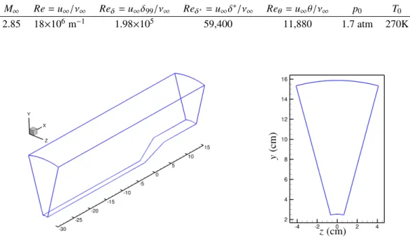
The flow conditions used in this study are listed in Table 1, and match the experiments of Dunagan et al. [23]. The incoming freestream Mach number is 2.85, and the Reynolds number based on freestream properties and momentum thickness (Reθ =u∞θ/ν∞) is about 11,880 based on a displacement thickness (δ∗) of 0.33 cm reported in Settles & Dodson [12] and assuming a shape factor (H=δ∗/θ) of≈5 (based on the results of Duan et al. [33]). FIgure 3 depicts

the computational domain used in this study. The azimuthal extent of the axisymmetric domain was either 30◦_{or 90}◦ for the grids used with periodic boundary conditions, and the effect of domain spanwise width is reported in Section IV.C.3. The spanwise extent (arc length) of the domain along the surface upstream of the corner is 1.33 cm (for 30◦₎ and 3.99 cm (for 90◦_{), and the incoming boundary layer isδ}

99=1.1 cm atx=-4.5 cm. The compression corner is

located atx=0 cm, and the radius of the model upstream of the corner is 2.54 cm. The length of the model between the

compression and expansion corners in the experiment was 6 cm (along the inclined model surface). Thus, for a 30◦ angle, the expansion corner is located atx=5.196 cm (6 cm×cos30◦). The inflow of the domain is located atx=−30

cm and the outflow is placed atx=15 cm. The experimental wind tunnel wall was rectangular with a width of 25.4 cm

and height of 38.1 cm. To approximately account for the presence of wind tunnel walls, we assume an axisymmetric tunnel wall with a diameter of 32 cm ((25.4+38.1)/2). Note that if we had matched the cross-sectional area of the tunnel, the diameter would have instead been 35.1 cm (πD2/4=25.4×38.1). RANS simulations indicated a negligible

Table 1 Flow conditions for the shock/ turbulence interaction problem under study matching the experiments of Dunagan et al. [23] The values ofReδ andReδ∗ are at a station upstream of the compression corner based

onδ₉₉=1.1 cm andδ∗_{=0.33 cm, and are taken from the shock/boundary layer interaction database of Settles} & Dodson [12]. Reθ is computed assumingH =δ∗/θof 5, which is estimated based on the turbulent boundary layer data of Duan et al. [33]

M∞ Re=u∞/ν∞ Reδ =u∞δ₉₉/ν∞ Reδ∗=u_∞δ∗/ν_∞ Re_θ =u_∞θ/ν_∞ p₀ T₀

2.85 18×106m−1 1.98×105 59,400 11,880 1.7 atm 270K

z(cm)

y

(cm)

Fig. 3 The computational domain used in this study corresponding to an azimuthal extent of 30◦is shown. The entire domain (left) and the inflow plane (right) are depicted.

difference between the results using the two diameters. We impose inviscid slip wall boundary conditions to mimic the effects of the tunnel wall. Note that DeBonis [25] placed the tunnel wall at≈52 cm and imposed characteristic-based

freestream boundary conditions. The effect of tunnel wall boundary conditions is discussed in Section IV.C.2. A sponge boundary condition is applied at the outflow boundary with a sponge region length of 2 cm. Note that the shock exits the domain through the outflow boundary. A Dirichlet boundary condition (from LES) was used for the wall model at an exchange location of 0.08 cm above the wall for the coarse and medium grids, and 0.093 cm above the wall for the fine grid.

The velocity and turbulent stress profiles at x = -4.5 cm and density profiles at x = -5.030 cm from the experiment were rescaled (based on turbulent boundary layer thickness dependence on distance from leading edge) to x = -30 cm to impose inflow boundary conditions (see Section III.B). Synthetic inflow turbulence was generated using the method of Shur et al. [34] with 405 modes and a wavenumber geometric ratio of 1.01. The thermodynamic fluctuations were prescribed based on the Strong Reynolds Analogy for temperature and density. The simulations were run for≈180 δ₉₉/u∞(δ99=1.1 cm) to flush out transients after which statistics were collected for≈180δ99/u∞. The results are also averaged along the span. The difference between the statistics collected after 90 and 180δ₉₉/u∞was under 2% for the separation bubble length (fine grid result). The initial condition for the coarse grid simulations were free-stream conditions, while the medium and fine grid simulations were started with interpolated coarse grid results. Time-averaged Mach number contours are shown in the vicinity of the compression corner in Figure 4 for the coarse grid. Shocks are produced at separation and reattachment which occur in the experiment atx≈-2.73 cm and 0.97 cm, respectively. The

separation bubble region (x≈-3 cm to 1 cm ) is seen to be fully subsonic.

A. Grid Details

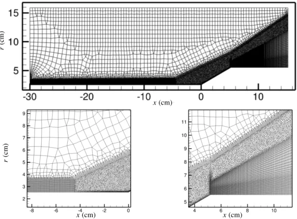
Figure 5 depicts the computational grid for the coarse grid in the symmetry plane (z=0). The grid in the entire

domain and in the vicinity of the compression and expansion corners are shown in the figure. The grid is unstructured and composed mostly of quadrilateral elements (in 2D). The symmetry plane grid is extruded in the azimuthal direction

x(cm)

r

(cm)

Fig. 4 Time-averaged Mach number (M) contours are shown in the symmetry plane (z =0). The incoming free-stream Mach number is 2.85.

Table 2 Grid spacings are listed atx=-5 cm. Here,δis the local boundary layer thickness from the experiment. The superscript ‘+’ denotes the viscous wall spacing computed based on aCf =0.0016 andTw/T∞ ≈2.62. All lengths are in cm. Note that the medium grid has the same spacings as the coarse grid at this location.

Grid ∆x,∆yw,∆zw ∆x+,∆y+w,∆z+w δ Nx/δ,Ny/δ,Nz/δ coarse 0.050, 0.052, 0.022 50, 52, 22 1.1 22, 21, 50

fine 0.016, 0.026, 0.011 16, 26, 11 1.1 68, 42, 100

to generate the 3D grid. It can be observed that only regions of activity such as boundary layer, separation bubble and shocks are refined while other regions of the flow are quickly coarsened to reduce the grid count. The grid spacings upstream of the compression corner are shown in Table 2. Three grids are used in this study: a coarse grid with≈6

million elements, medium grid with≈10 million elements, and a fine grid with≈42 million elements. The medium

grid has the same grid resolution as the coarse grid upstream of the separation bubble but is refined in the vicinity of the bubble. A snapshot of the coarse and medium grids upstream of the separation bubble is shown in Figure 6. While the coarse grid is unstructured in the vicinity of the wall, the medium grid is orthogonal to the wall until the edge of the boundary layer. The non-orthogonal nature of the coarse grid near the wall gave point-to-point oscillations in the skin friction from the wall model, and so the medium and fine grids were made orthogonal to the wall everywhere. Since the near-wall region is modeled in this study, the grid is fairly coarse in the wall-normal direction near the wall. The viscous wall spacings (∆x+_i =∆xiuτ/νw) are of the order of 50 and 20 for the coarse and fine grids, respectively. The coarse and fine grids were designed to contain at least 203_{and 40}3 _{grid points within a cube of the dimension of the local} boundary layer thickness.

B. Inflow Profiles

The leading edge of the model was at x=−100 cm (see Figure 2) in the experiment, and the earliest available

velocity and stress data are atx =−4.5 cm while the density data are atx =−5.03 cm. We decided to place the

inflow of the computational domain for WMLES simulations atx=−30 cm to provide sufficient streamwise distance

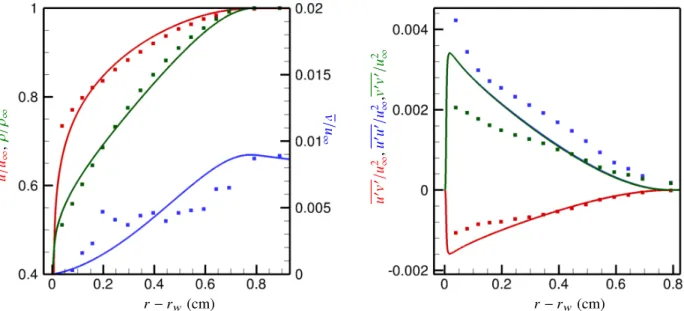
(over 30δ₉₉,i n) for the synthetic turbulence imposed at the inflow to develop into realistic turbulence. The velocity, stresses and density from the experiment at the earliest available location (-4.5 cm for velocity/ stresses, and -5.03 cm for density) were rescaled assuming a turbulent boundary layer from the leading edge based on the standard correlation (δ₉₉/x∼cRe−_x0.2, wherecis a constant of proportionality). Since only the outer layer is resolved in WMLES, we use a

single length scale, i.e., the ratio ofδ₉₉which is obtained from the correlation assuming the leading edge of the model to be atx=−100 cm, to rescale and obtain the profiles atx=−30 cm. Figure 7 compares the velocity, stress and density

x(cm) r (cm) x(cm) x(cm) r (cm)

Fig. 5 The computational grid in symmetry plane (z=0) of the entire computational domain (top), upstream

(bottom-left) and downstream (bottom-right) of the compression corner is shown in the figure for the coarse grid.

x(cm)

r

(cm)

Fig. 6 Grid upstream of the separation bubble for the coarse (red color) and medium (blue color) grids. Note the unstructured nature of the coarse grid in the vicinity of the wall.

thus validating the rescaling procedure. Note that the RANS inflow plane was placed atx=−75 cm (based on the

results of DeBonis [25]) to best match with the experimental profiles upstream of the separation bubble. Note that the SA-RANS does not capture the normal stresses accurately, and predicts the sameu0_u0_andv0_v0_{(which are proportional} tou0_v0_). r−rw (cm) u / u∞ , ρ/ ρ∞ v/ u ∞ r−rw (cm) u 0v 0/u 2,∞ u 0u 0/u 2,∞ v 0v 0/u 2 ∞

Fig. 7 Mean velocity and density variation (left), and Reynolds stresses variation (right) at the inflow plane of the computational domain (x=−30cm). The solid lines are from SA-RANS, and symbols are the rescaled experimental data from the earliest available station upstream of the separation bubble (x=−4.5cm for velocity and stresses, andx=−5.03cm for density). The color of the curve indicates the quantitity represented.

IV. Results

Qualitative and quantitative comparisons with available experimental data and RANS simulation are reported. The experimental data for comparison were taken from the shock/turbulence database of Settles & Dodson [12] and were provided to us in digitized form by DeBonis†_{. The instantaneous vortical features of the flow in the vicinity of the} compression corner are shown in Figure 8 using isocontours of the Q-criterion colored by instantaneous streamwise velocity for the fine grid. Coherent hairpin vortices in the upstream boundary layer and relatively larger scale features downstream of separation are observed in the figure. The separation bubble region with a lower streamwise velocity is clearly visible in the figure. For the results presented in this section, the coarse, medium and fine grid simulations are referred to as cWMLES, mWMLES and fWMLES, respectively. The fine grid results are currently only available for the equilibrium wall model. The equilibrium and non-equilibrium wall model results are referred to as EQWM and NEQWM, respectively.

A. Qualitative Comparisons with Experiment

Figure 9 compares the shadowgraph taken from the experiments of Brown et al. [24] to the numerical schlieren (instantaneous density gradient magnitude contours) taken from the coarse and fine WMLES simulations using the equilibrium wall model. The separation and reattachment shocks are clearly visible in the simulations and qualitatively similar to the experimental shadowgraph. Downstream of reattachment, the shocks appear to coalesce into a single shock. This trend is consistent between the experiment and simulation. The shocks are more smeared in the coarse grid while they are more sharply captured in the finer grid. Also, a weak shock is seen upstream of separation in the experimental shadowgraph (denotedδ₀), whereas no such shock is observed in the simulations. This may an instantaneous phenomena as it is absent in the bottom portion of the experimental shadowgraph.

u/u∞

Fig. 8 Instantaneous isocontours of the Q-criterion colored by instantaneous horizontal velocity (u/u∞) is shown to depict the vortical features in the vicinity of the compression corner from the fine grid simulation. Here, the dark blue region indicates upstream flow in the separation bubble.

fWMLES

cWMLES

Fig. 9 Shadowgraph image taken from Brown et al. [24] depicting the separation and reattachment shocks (left) and numerical Schlieren (density gradient magnitude) contour on the right from WMLES. The coarse (right-bottom) and fine (right-top) grid results are shown.

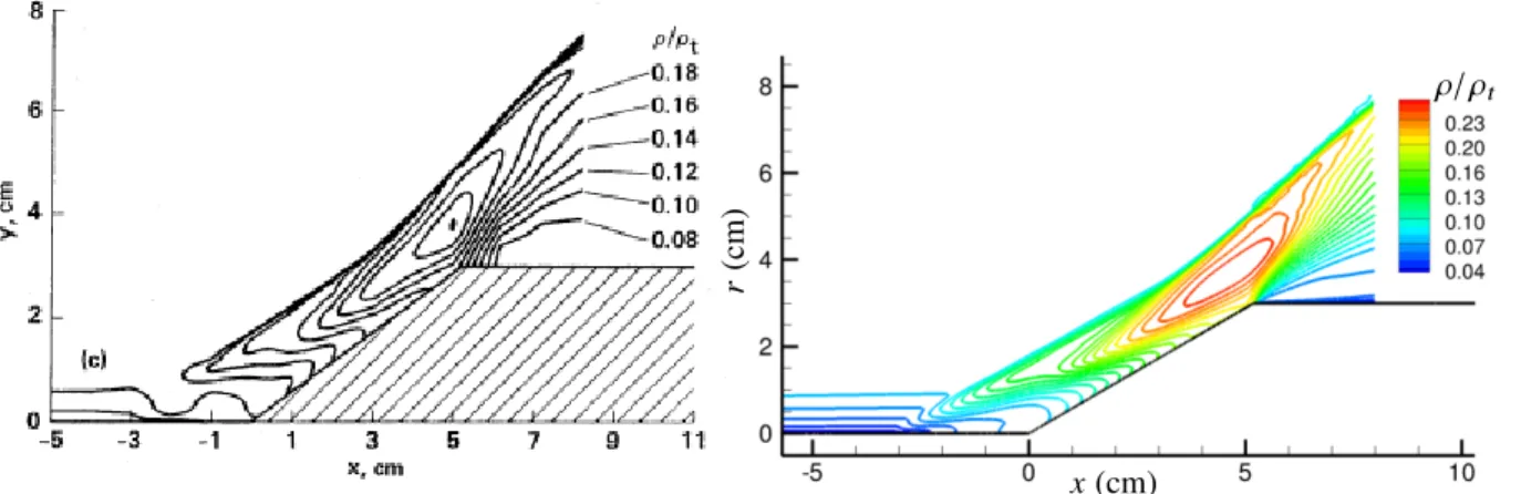
Figure 10 compares the time-averaged density contour lines obtained from interferometry by Dunagan et al. [23] and from the fine grid WMLES simulation using the equilibrium wall model. Overall, the contour lines appear qualitatively similar. However, some differences can be observed. The experiment appears to indicate that the peak density location occurs closer to the expansion corner, while the simulation predicts the location to be a bit upstream of the expansion corner. Also, the shape of the contour lines in the vicinity of separation (x=-3 to -1 cm) appears to exhibit some minor

differences.

x(cm)

r

(cm)

ρ/ρt

Fig. 10 Time-averaged density contour lines from experiments of Dunagan et al. [23] (left) and fWMLES (right).

B. Quantitative Comparisons with Experiment

In order to highlight the predictive ability of WMLES, we make detailed comparisons with available experimental data for the coarse (EQWM and NEQWM), and fine grids (EQWM). We compare the wall pressure variation; velocity, stresses and density profiles at various locations in the flow; and the separation bubble length. RANS predictions using the Spalart-Allmaras model (SA-RANS) are also shown to compare the predictions of WMLES with RANS. The sensitivity of the WMLES results to grid refinement, domain span, wall model exchange location are discussed in Section IV.C. The coarse grid results reported here use a span of 30◦_{, while the fine grid results used a span of 90}◦_{. The} effect of spanwise width between 30◦_{and 90}◦_{are negligible (see Section IV.C.3).}

Figure 11 shows the variation of mean wall pressure variation with the streamwise coordinate for the coarse and fine grid equilibrium WMLES simulations (cWMLES and fWMLES), coarse grid non-equilibrium wall model results (cWMLES-NEQWM), SA-RANS and experiments of Dunagan et al. [23]. Overall, the cWMLES-NEQWM simulation agrees best with experiment, with fWMLES also doing reasonably well. However, refinement of the grid for the NEQWM made the agreement worse with experiment (see Section IV.C.4). Overall, the agreement with experiment for wall pressure prediction is comparable to SA-RANS.

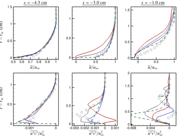
The time-averaged horizontal velocity and turbulent shear stresses are compared with SA-RANS and experiment at three locations upstream of the compression corner in Figure 12. Note thatu0_v0_{is along the horizontal (x) and radial (r)} directions. In the experiment, the flow separates atx=-2.73 cm, and so we chose locations upstream of separation, near

separation and within the separation bubble. The earliest experimental velocity and stress data are atx=-4.5 cm, and

good agreement is observed between WMLES, SA-RANS and experiment at this location. Except very near the wall (where the experiment may be inaccurate), the agreement in turbulent shear stress is good. Differences between the wall models are evident atx=-3 cm, where again the non-equilibrium wall model result agrees best with experiment.

Since the fWMLES simulation separates a bit further upstream of the cWMLES-NEQWM, the velocity profile is closer to separation at this location, and deviates more from experiment, which separates at -2.73 cm. Atx=-1 cm, all the

three wall models deviate from experiment in the near-wall region. Overall, the cWMLES-NEQWM agrees best with experiment, followed by the fWMLES result.

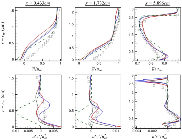
The time-averaged horizontal velocity and turbulent shear stresses are compared with SA-RANS and experiment at three locations downstream of the compression corner in Figure 13. At locations closer to the corner, there is a noticeable disagreement with experiment for all the WMLES results (and SA-RANS) similar to what was observed upstream of the corner. Overall, the agreement for all the WMLES simulations in velocity profiles is comparable to

x(cm)

p

/ρ∞

u

2 ∞

Fig. 11 Mean wall pressure variation is compared to experiment. Legend: cWMLES, cWMLES-NEQWM, fWMLES, SA-RANS, andDunagan et al. experiment [23].

r − rw (cm) u/u∞ x=−4.5 cm u/u∞ x=−3.0 cm u/u∞ x=−1.0 cm r − rw (cm) u0_v0/_u2 ∞ u0v0/u∞2 u0v0/u2∞

Fig. 12 Profiles of time-averaged horizontal velocity (u), vertical velocity (v) and Reynolds shear stress (u0_v0₎ are compared to the experiment and RANS at locations upstream of the compression corner. Legend: cWMLES, cWMLES-NEQWM, fWMLES, SA-RANS, andDunagan et al. experiment [23].

SA-RANS. However, the WMLES results show superior predictions in the turbulent shear stress at these locations. At

x=1.732 cm, SA-RANS still predicts a negative turbulent shear stress and takes a long distance downstream to recover

to the correct profile.

u/u∞ r − rw (cm) x=0.433cm u/u∞ x=1.732cm u/u∞ x=5.896cm u0_v0_/u2 ∞ r − rw (cm) u0_v0_/u2 ∞ u0v0/u2∞

Fig. 13 Profiles of time-averaged horizontal velocity (u), vertical velocity (v) and Reynolds shear stress (u0_v0₎ are compared to the experiment and RANS at locations downstream of the compression corner. Legend: cWMLES, cWMLES-NEQWM, fWMLES, SA-RANS, andDunagan et al. experiment [23].

Time-averaged density profiles are compared to experiment in Figure 14 at locations upstream and downstream of the compression corner. Atx=-5.03 cm, both WMLES and SA-RANS predict a larger boundary layer thickness

based on 99% of the free-stream density compared to experiment. Also, the boundary layer edge density predicted by WMLES is 0.975 instead of 1 in the experiment. The exact reason for this is unclear. Over all the locations, the cWMLES-NEQWM and fWMLES perform better compared to experiment than cWMLES. Also, the level of agreement with experiment in density profiles is comparable to RANS.

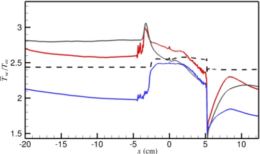
Overall, in terms of wall pressure, velocity, stresses and density, it was seen the cWMLES-NEQWM simulation agreed best with experiment followed by fWMLES and cWMLES. It should be noted that predicting the correct separation bubble size is critical to match other quantities in the separation bubble. Also, since we applied an adiabatic wall boundary condition, we compare the wall temperature returned by the wall models with SA-RANS in Figure 15. Note that no experimental data is available for temperature variation. For attached regions of the flow, the theoretical adiabatic wall temperature (Tw,ad/T∞ =1+0.5(γ−1)r M∞) assuming a recovery factor (2 r) of 0.85 is 2.381 for a free-stream Mach number of 2.85. SA-RANS predicts a wall temperature of≈2.42 which is close to the theoretical

value, but the WMLES predicts upstream wall temperatures between 2.1 and 2.8 with up to 17% error.

The mean streamlines in the vicinity of the separation bubble are shown for the cWMLES simulation in Figure 16. The flow separates atx≈-3.1 cm and reattaches atx≈1 cm in the figure, which is close to the experimental values of

-2.7 cm and 0.97 cm obtained from oil flow visualization [23]. Table 3 lists the separation and reattachment locations for the WMLES simulations, SA-RANS and SST-RANS from DeBonis [25], and experiment. The experimental separation and reattachment locations are from oil flow visualization and are only approximate [23, 35]. The separation and reattachment locations are extracted from the mean streamlines in WMLES. Note that if the exchange location for the wall model is placed away from the first grid point from the wall, the skin friction returned by the wall model will be

r − rw (cm) ρ/ρ∞ x=−5.030 cm ρ/ρ∞ x=−3.009 cm ρ/ρ∞ x=−1.007 cm r − rw (cm) ρ/ρ∞ x=0.996 cm ρ/ρ∞ x=2.996 cm ρ/ρ∞ x=6.173 cm

Fig. 14 Profiles of time-averaged density (ρ) are compared to the experiment and RANS at locations upstream of the compression corner. Legend: cWMLES, cWMLES-NEQWM, fWMLES, SA-RANS, and

Dunagan et al. experiment [23].

x(cm) Tw

/

T∞

Fig. 15 Mean wall temperature variation is compared to SA-RANS. Legend: cWMLES,

Table 3 Separation bubble characteristics from the simulations and experiment. All dimensions are in cm. For the equilibrium wall model results with exchange location away from the wall, the separation and reattachment locations were calculated based on the near-wall velocity vector.

xS xR LB Error in bubble length

Experiment [23] -2.73 0.97 3.7 – cWMLES-EQWM -3.06 1.33 4.39 18.65% cWMLES1-EQWM -2.97 1.08 4.05 9.46% mWMLES-EQWM -2.26 0.73 2.99 -19.19% fWMLES-EQWM -2.88 1.05 3.93 6.2% cWMLES-NEQWM -2.85 1.27 4.12 11.35% mWMLES-NEQWM -2.06 0.7 2.76 -25.41% SA-RANS [25] -2.67 2.27 4.92 32.9% SST-RANS [25] -4.57 2.54 7.11 92.1%

aligned with the velocity vector at the exchange location, which could be different (and typically is in separated regions from our experience) from the near-wall velocity vector represented by streamlines. A similar observation was also made by Dawson et al. [36]. The cWMLES1-EQWM uses the first grid point as the exchange location, and an integral constraint boundary condition instead of the Dirichlet boundary conditions (see IV.C.1 for details of the boundary conditions) used by all the other WMLES simulations reported. The error in bubble length prediction compared to the experimental value is also reported. The fWMLES simulation agrees best with experiment with a 6% error in bubble length, while the coarse grid simulations have≈10%−25% error. Interestingly, the medium grid (finer only in the

vicinity of the separation bubble compared to the coarse grid) underpredicts the bubble size for both wall models with an error of the order of 20%. Also, the medium grid gives worse predictions compared to the coarse grid for the NEQWM simulations. Note that DNS results of Wu and Martin [22] predicted a 10% smaller separation bubble for a lowRe

compression ramp configuration compared to the experiments of Bookey et al. [37] in spite of the fine resolution, and matching all quantities upstream of the bubble. Thus, the separation bubble length in a shock/ boundary layer interaction is quite challenging to predict even for DNS, and so a 6% error for the fWMLES simulation should be considered good in this context. Also, it is difficult to assess the quality of WMLES prediction with respect to bubble length without more accurate experimental data. Note that the bubble length predictions by RANS are significantly more erroneous compared to WMLES, although RANS predicted reasonable velocity and density profiles at the locations compared.

x(cm)

r

(cm)

C. Sensitivity of Results

In an effort to narrow down possible reasons for discrepancies in the WMLES predictions, we explore the sensitivity of the results to various parameters in this section. The effect of exchange location, tunnel wall confinement, spanwise extent of the domain, and grid refinement are discussed. Most of the sensitivities are explored using the coarse grid. The mean wall pressure and skin friction coefficient are reported to depict sensitivity to various parameters.

1. Effect of Exchange Location

When the exchange location is placed away from the near-wall grid point based on suggestion of Kawai and Larsson [5], a Dirichlet boundary condition is applied on the wall model using information from LES. On the other hand, when the near-wall grid point (1st grid point) is used as the exchange location, an integral constraint boundary condition can also be used. The Dirichlet boundary condition for the wall model is:

uw m|ηm a x = uL E S|ηm a x (1)

whereηma xis the location of the farthest wall model grid point. The integral constraint boundary condition is: 1

ηma x

Z ηm a x

0 uw md

η = uL E S|ηm a x/2 (2)

with an analogous boundary condition for temperature. In our previous study of an axisymmetric transonic bump configuration [28], the integral constraint boundary condition gave superior wall pressure predictions, and so we report the differences between using the two different boundary conditions for the coarse grid using the equilibrium wall model. cWMLES1 refers to the coarse grid simulation using the intergral boundary condition and the 1st near wall grid point as exchange location. cWMLES refers to the simulation using the dirichlet boundary condition at an exchange location 0.08 cm from the wall. The wall pressure and skin friction variation is shown in Figure 17. Some differences in wall pressure can be observed in the vicinity of separation and downstream of reattachment. Both the simulations predict identical skin friction far upstream, likely indicating that there is no log-layer mismatch. However, both simulations underpredict the skin friction (C f ≈0.0014) compared to SA-RANS predictions (Cf ≈0.0017) with an error of≈18%. This underprediction ofCf was also observed in our previous study at transonic conditions [28], and might be related to errors from the inflow turbulence generation and/or wall model. Another prominent feature visible in the skin friction plot is the oscillations in theCf curve for the cWMLES1 case. This appears to be due to unstructured nature of the grid in the vicinity of the wall depicted in Figure 6. However, theCf curve is smooth when a fixed exchange location is used at a grid point away from the wall. Thus, it appears that apart from minimizing log-layer mismatch errors in attached flows [5], using information away from the wall also provides smoother results when unstructured grids are used.

x(cm) pw /ρ∞ u 2 ∞ x(cm) Cf

Fig. 17 Mean wall pressure (left) and skin friction (right) variation showing the effect of exchange location for the coarse grid. Legend: cWMLES1, cWMLES, SA-RANS andDunagan et al. experiment [23].

2. Effect of Tunnel Wall Confinement

In our simulations, we use an inviscid slip wall BC atr=16 cm to mimic tunnel wall effects in the experiment.

To assess the effect of tunnel wall confinement, we also perform a simulation with the top wall boundary located at

r=52 cm and impose free-stream reference boundary conditions. These simulations use the coarse grid with 1st grid

point as exchange location as evident from the oscillations in theCf variation in Figure 18. The effect of tunnel wall confinement is negligible for predicting skin friction, and also small for the wall pressure variation except close to the expansion corner. x(cm) pw /ρ∞ u 2 ∞ x(cm) Cf

Fig. 18 Mean wall pressure (left) and skin friction (right) variation showing the effect of tunnel wall confinement for cWMLES1. Legend: Inviscid Slip Wall BC atr=16 cm, Free-stream BC atr≈52cm, SA-RANS andDunagan et al. experiment [23].

3. Effect of Domain Spanwise Extent

Figure 19 shows the effect of the spanwise domain extent (30◦_{vs. 90}◦_{) on the mean wall pressure and skin friction} coefficient for the cWMLES1 simulation. The results suggest that the influence of spanwise extent of the domain is negligible. Note that the upstream boundary layer thickness is≈1.1 cm, and the spanwise extent of the domain along the

surface at the wall upstream of the corner is 1.33 cm (and increases as we move away from the wall since the geometry is axisymmetric). In spite of the the spanwise extent being of the order of the upstream boundary layer thickness, it is interesting that the mean wall pressure and skin friction are well-captured. Spanwise correlations of velocity and pressure will be analyzed in the future to verify this observation.

x(cm) pw /ρ∞ u 2 ∞ x(cm) Cf

Fig. 19 Mean wall pressure (left) and skin friction (right) variation showing the effect of spanwise domain width. Legend: 30◦_{, 90}◦_{, SA-RANS, and}

4. Effect of Grid Refinement

The effect of grid refinement for the equilibrium wall model is shown in Figure 20. The exchange location is 0.08 cm from the wall for the coarse and medium grids, and 0.093 cm for the fine grid. The wall pressure and skin friction results indicate that the grid refinement has a noticeable effect on the results. Upstream of the compression corner, the

Cf for all the three grids are in good agreement with each other indicating that the lowerCf compared to SA-RANS is not related to the grid resolution. Good agreement inCf for the non-equilibrium wall model ( Figure 21) for the same inflow turbulence generation technique suggests that the difference may not be due to the inflow turbulence generation technique as well. Overall, the fine grid results agree best with experiment in terms of the wall pressure, and bubble size (reported in Table 3). Note that the separation bubble length would be significantly smaller if computed based on the mean skin friction, sinceCf is parallel to the velocity vector at the exchange location.

x(cm) pw /ρ∞ u 2 ∞ x(cm) Cf

Fig. 20 Mean wall pressure (left) and skin friction (right) variation showing the effect of grid refinement using the EQWM. Legend: cWMLES, mWMLES, fWMLES, SA-RANS andDunagan et al. experiment [23].

The effect of grid refinement for the non-equilibrium wall model is shown in Figure 21. The exchange location (0.08 cm) is identical to the equilibrium wall model case. The coarse grid gives excellent agreement with experiment for the wall pressure prediction, but deviates from experiment as the grid is refined in the vicinity of the separation bubble. Worsening of the predictions from coarse to medium grids was also observed for the equilibrium wall model. The wall skin friction agrees well with SA-RANS far upstream. In the vicinity of the separation bubble and downstream of it, the coarse grid exhibits oscillations similar to the cEQWM1 results. Although the exchange location was the same for the cEQWM and cNEQWM simulations, the cNEQWM exhibits oscillations in the skin friction predictions. It is unclear whether this is due to interpolation errors at the exchange location.

x(cm) pw /ρ∞ u 2 ∞ x(cm) Cf

Fig. 21 Mean wall pressure (left) and skin friction (right) variation showing the effect of grid refinement using the NEQWM. Legend: cWMLES, mWMLES, SA-RANS andDunagan et al. experiment [23].

V. Summary

Wall-modeled Large Eddy Simulation (WMLES) were performed for a highReaxisymmetric, supersonic compression

ramp geometry at conditions matching experiments of Dunagan et al. [23]. Detailed comparisons were made with available experimental data including wall pressure, velocity, density and turbulent stress profiles along with separation bubble length. The finest grid overall gave good agreement with experiment with about 6% error in the bubble length prediction. The coarser grids gave larger errors (10−25%) in predicting separation bubble length depending on the

grid and wall model used. Sensitivity of the WMLES results to grid resolution, type of wall model (equilibrium or non-equilibrium), wall model exchange location, tunnel wall boundary condition, and spanwise width of the domain were explored, and the results were relatively insensitive to the latter three parameters for the coarse grid in terms of the mean wall pressure and skin friction. When compared to RANS (using the SA model for the present configuration), WMLES provides improved prediction of the separation bubble length and turbulent shear stress profiles downstream of the compression corner.

Acknowledgments

This research was sponsored by the NASA Transformational Tools and Technologies (TTT) Project of the Transformative Aeronautics Concepts Program under the Aeronautics Research Mission Directorate. The work of the first author was sponsored by NASA under cooperative agreement NNL09AA00A. We thank Cascade Technologies for providing the Charles solver and consultation in use of the code, Dr. George Park for help with the non-equilibrium model version of the code, Dr. Jim DeBonis for the grid used in the RANS simulations and experimental data, and Dr. Balaji Venkatachari for valuable discussions.

References

[1] Larsson, J., Kawai, S., Bodart, J., and Bermejo-Moreno, I., “Large eddy simulation with modeled wall-stress: recent progress

and future directions,”Mechanical Engineering Reviews, Vol. 3, No. 1, 2016, pp. 15–00418.

[2] Bose, S. T., and Park, G. I., “Wall-Modeled Large-Eddy Simulation for Complex Turbulent Flows,”Annual Review of Fluid

Mechanics, Vol. 50, No. 1, 2018, pp. 535–561.

[3] Cabot, W., and Moin, P., “Approximate wall boundary conditions in the large-eddy simulation of high Reynolds number flow,”

Flow, Turbulence and Combustion, Vol. 63, No. 1–4, 2000, pp. 269–291.

[4] Piomelli, U., and Balaras, E., “Wall-layer models for large-eddy simulations,”Annual Review of Fluid Mechanics, Vol. 34,

No. 1, 2002, pp. 349–374.

[5] Kawai, S., and Larsson, J., “Wall-modeling in large eddy simulation: Length scales, grid resolution, and accuracy,”Physics of

Fluids, Vol. 24, No. 1, 2012, p. 015105.

[6] Kawai, S., and Larsson, J., “Dynamic non-equilibrium wall-modeling for large eddy simulation at high Reynolds numbers,”

Physics of Fluids, Vol. 25, No. 1, 2013, p. 015105.

[7] Park, G. I., and Moin, P., “An improved dynamic non-equilibrium wall-model for large eddy simulation,”Physics of Fluids,

Vol. 26, No. 1, 2014, p. 015108.

[8] Bose, S., and Moin, P., “A dynamic slip boundary condition for wall-modeled large-eddy simulation,”Physics of Fluids, Vol. 26,

No. 1, 2014, p. 015104.

[9] Yang, X., Sadique, J., Mittal, R., and Meneveau, C., “Integral wall model for large eddy simulations of wall-bounded turbulent

flows,”Physics of Fluids, Vol. 27, No. 2, 2015, p. 025112.

[10] Spalart, P. R., “Detached-eddy simulation,”Annual Review of Fluid Mechanics, Vol. 41, 2009, pp. 181–202.

[11] Shur, M. L., Spalart, P. R., Strelets, M. K., and Travin, A. K., “A hybrid RANS-LES approach with delayed-DES and

wall-modelled LES capabilities,”International Journal of Heat and Fluid Flow, Vol. 29, No. 6, 2008, pp. 1638–1649.

[12] Settles, G. S., and Dodson, L. J., “Hypersonic shock/boundary-layer interaction database,” NASA-CR-177577, 1991.

[13] Andreopoulos, Y., Agui, J. H., and Briassulis, G., “Shock wave–turbulence interactions,”Annual Review of Fluid Mechanics,

[14] Knight, D., Yan, H., Panaras, A. G., and Zheltovodov, A., “Advances in CFD prediction of shock wave turbulent boundary layer

interactions,”Progress in Aerospace Sciences, Vol. 39, No. 2, 2003, pp. 121–184.

[15] Gaitonde, D. V., “Progress in shock wave/boundary layer interactions,”Progress in Aerospace Sciences, Vol. 72, 2015, pp.

80–99.

[16] Settles, G. S., Vas, I. E., and Bogdonoff, S. M., “Details of a shock-separated turbulent boundary layer at a compression corner,”

AIAA Journal, Vol. 14, No. 12, 1976, pp. 1709–1715.

[17] Dolling, D., and Murphy, M., “Unsteadiness of the separation shock wave structure in a supersonic compression ramp flowfield,”

AIAA Journal, Vol. 21, No. 12, 1983, pp. 1628–1634.

[18] Smits, A. J., and Muck, K.-C., “Experimental study of three shock wave/turbulent boundary layer interactions,”Journal of

Fluid Mechanics, Vol. 182, 1987, pp. 291–314.

[19] Adams, N. A., “Direct numerical simulation of turbulent compression ramp flow,”Theoretical and Computational Fluid

Dynamics, Vol. 12, No. 2, 1998, pp. 109–129.

[20] Rizzetta, D. P., Visbal, M. R., and Gaitonde, D. V., “Large-eddy simulation of supersonic compression-ramp flow by high-order

method,”AIAA Journal, Vol. 39, No. 12, 2001, pp. 2283–2292.

[21] Loginov, M. S., Adams, N. A., and Zheltovodov, A. A., “Large-eddy simulation of shock-wave/turbulent-boundary-layer

interaction,”Journal of Fluid Mechanics, Vol. 565, 2006, pp. 135–169.

[22] Wu, M., and Martin, M. P., “Direct numerical simulation of supersonic turbulent boundary layer over a compression ramp,”

AIAA journal, Vol. 45, No. 4, 2007, pp. 879–889.

[23] Dunagan, S. E., Brown, J. L., and Miles, J. B., “Interferometric data for a shock-wave/boundary-layer interaction,” NASA-TM-101008, 1986.

[24] Brown, J. D., Brown, J., and Kussoy, M. I., “A documentation of two-and three-dimensional shock-separated turbulent boundary layers,” NASA-TM-101008, 1988.

[25] DeBonis, J. R., “Evaluation of Industry Standard Turbulence Models on an Axisymmetric Supersonic Compression Corner,” AIAA Paper 2015-314, 2015.

[26] Bermejo-Moreno, I., Campo, L., Larsson, J., Bodart, J., Helmer, D., and Eaton, J. K., “Confinement effects in shock

wave/turbulent boundary layer interactions through wall-modelled large-eddy simulations,”Journal of Fluid Mechanics, Vol.

758, 2014, pp. 5–62.

[27] Iyer, P. S., and Malik, M. R., “Wall–Modeled Large Eddy Simulation of Flow Over a Wall–Mounted Hump,” AIAA Paper 2016–3186, 2016.

[28] Iyer, P. S., Park, G. I., and Malik, M. R., “Wall–Modeled Large Eddy Simulation of Transonic Flow over an Axisymmetric Bump with Shock-Induced Separation,” AIAA Paper 2017-3953, 2017.

[29] Khalighi, Y., Ham, F., Nichols, J., Lele, S., and Moin, P., “Unstructured large eddy simulation for prediction of noise issued from turbulent jets in various configurations,” AIAA Paper 2011-2886, 2011.

[30] Brès, G. A., Ham, F. E., Nichols, J. W., and Lele, S. K., “Unstructured Large-Eddy Simulations of Supersonic Jets,”AIAA

Journal, Vol. 55, No. 4, 2017, pp. 1164–1184.

[31] Biedron, R. T., Carlson, J. R., Joseph, M. D., Gnoffo, P. A., Hammond, D. P., Jones, W. T., Kleb, B., Lee-Rausch, E. M., Nielsen, E. J., Park, M. A., Rumsey, C. L., Thomas, J. L., and Wood, W. A., “FUN3D Manual: 13.1,” NASA-TM-2019580, 2017. [32] Sfeir, A. A., “Supersonic Laminar Boundary Layer Separation Near a Compression Corner,” Report No. AS-69-6, CALIFORNIA

UNIV BERKELEY DIV OF AERONAUTICAL SCIENCES, 1969.

[33] Duan, L., Beekman, I., and Martin, M., “Direct numerical simulation of hypersonic turbulent boundary layers. Part 3. Effect of

Mach number,”Journal of Fluid Mechanics, Vol. 672, 2011, pp. 245–267.

[34] Shur, M. L., Spalart, P. R., Strelets, M. K., and Travin, A. K., “Synthetic turbulence generators for RANS-LES interfaces in

zonal simulations of aerodynamic and aeroacoustic problems,”Flow, Turbulence and Combustion, Vol. 93, No. 1, 2014, pp.

[35] Dunagan, S. E., Brown, J., and Miles, J., “Holographic interferometry study of an axisymmetric shock-wave/boundary-layer

strong interaction flow,”AIAA Journal, Vol. 25, No. 2, 1987, pp. 294–299.

[36] Dawson, D. M., Lele, S. K., and Bodart, J., “Assessment of wall-modeled large eddy simulation for supersonic compression ramp flows,” AIAA Paper 2013-3638, 2013.

[37] Bookey, P., Wyckham, C., Smits, A., and Martin, P., “New experimental data of STBLI at DNS/LES accessible Reynolds numbers,” AIAA Paper 2005-309, 2005.