Incorporating Rich Features into Deep Knowledge Tracing

Worcester Polytechnic Institute

Digital WPI

Masters Theses (All Theses, All Years) Electronic Theses and Dissertations

2017-04-14

Incorporating Rich Features into Deep Knowledge

Tracing

Liang Zhang

Worcester Polytechnic Institute

Follow this and additional works at:https://digitalcommons.wpi.edu/etd-theses

This thesis is brought to you for free and open access byDigital WPI. It has been accepted for inclusion in Masters Theses (All Theses, All Years) by an authorized administrator of Digital WPI. For more information, please [email protected].

Repository Citation

Zhang, Liang, "Incorporating Rich Features into Deep Knowledge Tracing" (2017).Masters Theses (All Theses, All Years). 207.

Incorporating Rich Features into Deep Knowledge Tracing

Liang Zhang

A Thesis

Submitted to the Faculty of the

WORCESTER POLYTECHNIC INSTITUTE In partial fulfillment of the requirements for the

Degree of Master of Science in

Data Science by

April 2017 APPROVED:

Professor Neil T. Heffernan, Thesis Advisor

Professor Diane M. Strong, Reader

Abstract

The desire to follow student learning within intelligent tutoring systems in near real time has led to the development of several models anticipating the correctness of the next item as students work through an assignment. Such models have in-cluded Bayesian Knowledge Tracing (BKT), Performance Factors Analysis (PFA), and more recently with developments in Deep Learning, Deep Knowledge Tracing (DKT). The DKT model, based on the use of a recurrent neural network, exhibited promising results in paper [PBH+_15].

Thus far, however, the model has only considered the knowledge components of the problems and correctness as input, neglecting the breadth of other features col-lected by computer-based learning platforms. This work seeks to improve upon the DKT model by incorporating more features at the problem-level and student-level. With this higher dimensional input, an adaption to the original DKT model struc-ture is also proposed, incorporating an Autoencoder network layer to convert the input into a low dimensional feature vector to reduce both the resource requirement and time needed to train.

Experimental results show that our adapted DKT model, which includes more combinations of features, can effectively improve accuracy.

Acknowledgements

I would like to thank the following people who gave me help, support and sug-gestion in completing this dissertation. Joseph E. Beck, Jacob Richard Whitehill, Xiaolu Xiong, Siyuan Zhao and Anthony Botelho.

My committee member, Professor Diane M. Strong, helped to shape this disser-tation into its present form, taught me a great deal about data science knowledge, and gave me a lot of support to my study in WPI.

My advisor, Professor Neil T. Heffernan, is an exceptional mentor, and has guided me for a whole year in learning how to conduct research effectively and efficiently.

Finally, I would like to thank my wife, Ping Hao. She gave me more confidence to return school to do what I am excited in after working in industry for more than 10 years.

Contents

List of Figures iv

List of Tables v

1 Knowledge Tracing 1

1.1 Bayesian Knowledge Tracing . . . 2

1.2 Performance Factor Analysis . . . 4

1.3 Deep Knowledge Tracing . . . 5

2 Deep Learning 8 2.1 Deep Neural Network . . . 8

2.2 Recurrent Neural Network . . . 10

2.3 Autoencoder . . . 12

3 Improving DKT with More Features 15 3.1 Feature engineering . . . 16

3.1.1 Cross Features . . . 17

3.1.2 One-Hot Encoding . . . 17

3.1.3 Word Embedding . . . 19

3.1.4 Feature process . . . 21

3.3 Reduce dimension using Autoencoder . . . 27

3.4 DKT Extension Model . . . 29

3.5 Optimization . . . 30

4 Datasets and Environment 32 4.1 Datasets . . . 32 4.1.1 ASSISTments 2009-2010 . . . 33 4.1.2 OLI Statics F2011 . . . 34 4.2 Evaluation Metrics . . . 34 4.3 Running Environment . . . 35 5 Results 36 6 Discussion 39 6.1 Drawback in constructing skill graph . . . 39

6.2 Future work . . . 39

List of Figures

2.5 Encoder and Decoder. . . 13

2.6 Stacked Autoencoder . . . 14

3.1 weights above: separate features below: cross feature . . . 18

3.2 Wording Embedding in natural language process . . . 20

3.3 Time z-score (X axis) and Correctness (Y axis) . . . 23

3.4 Time z-score and correctness for different opportunity . . . 24

3.5 Time z-score and correctness for single skill . . . 25

3.6 Concatenated encoded features . . . 26

3.7 Undercomplete Autoencoder. . . 28

3.8 New DKT LSTM Model without Autoencoder . . . 29

3.9 New DKT LSTM Model with Autoencoder . . . 30

List of Tables

3.1 Student records example . . . 18

3.2 One-hot encoding . . . 19

3.3 One-hot encoding of cross features . . . 19

3.4 Simulated Word embedding representation of cross features . . . 20

3.5 Hyper parameter setting . . . 31

4.1 Dataset statistics information . . . 32

5.1 ASSISTments 2009 dataset Result . . . 36

Chapter 1

Knowledge Tracing

The goal of knowledge inference is to measure what relevant knowledge components a student knows at a specific time. Inferring student knowledge allows us to adapt to differences in what students know; for instance, if we believe that a student does not yet know the skill they are working on, more exercises can be given until he or she reach mastery. Although the knowledge component, which may be skill, fact, concept or principle, is not directly measurable, we can look at students’ performance at the knowledge component. Knowledge tracing models that attempt to follow the progression of student learning often represent student knowledge as a latent variable. As students work on new problems, these models update their estimates of student knowledge based on the correctness of responses. The problem is time series prediction, as student performance on previous items is indicative of future performance. Models then use the series of questions a student has attempted previously and the correctness of each question to predict the students performance on a new problem. In other words, the model predict the correctness of the next problem correctness (NPC). Two well-known models, Bayesian Knowledge tracing (BKT)[CA94] and Performance Factor Analysis(PFA) [JCK09] have been widely

explored due to their ability to capture this progression of knowledge with reliable accuracy. Both of these models exhibit success in terms of predictive accuracy but use different algorithms to estimate student knowledge

1.1

Bayesian Knowledge Tracing

Bayesian Knowledge Tracing (BKT), first suggested by Atkinson [1972][Atk72] and more thoroughly discussed by Corbett & Anderson [1995][CA94], is probably the most popular algorithm for modeling student learning. BKT is a simple Bayesian Network as well as being a first order Markov process. BKT attempts to assess the latent variable of the students knowledge state, using the students performance to make that inference. This model assumes that at any given opportunity to demon-strate a skill, the knowledge state of a student is a binary variable, mastered or not, and the observed performance is a correct or incorrect response. It updates the probability that the student has mastered the skill based on their performance on each opportunity to demonstrate the skill. In classical BKT, only the first at-tempt for each opportunity is taken into account, and it is assumed that each item corresponds to only a single skill. In its original formulation, a different set of four parameters is fit for each skill, the first two are learning parameters while the last two are performance parameters.

• P(L0) – probability the skill is already mastered before the first opportunity to use the skill in problem solving.

• P(T) – probability the skill will be learned at each opportunity to use the skill.

• P(S) – probability the student will make a mistake if the skill is mastered. The equations are used to infer student latent knowledge from performance. Actualn means the actual correctness of the exercise.

P(Ln−1|Correctn) = P(Ln−1∗(1−P(S))) P(Ln−1)∗(1−P(S)) + (1−P(Ln−1))∗P(G) (1.1) P(Ln|Incorrectn) = P(Ln−1)∗P(S) P(Ln−1)∗P(S) + (1−P(Ln−1)∗(1−P(G))) (1.2)

P(Ln|Actualn) = P(Ln−1|Actualn) + ((1−P(Ln−1|Actualn)∗P(T))) (1.3)

Both the expectation maximization algorithm and grid search have been used to estimate the parameters from training data. The assumption is made that students do not forgot a skill once they have learned it. Another assumption is that all items, within the same skill, have the same difficulty, and that no contextual factors (beyond what skill it is) impact student performance or learning.

The last decade has seen many different variants which attempt to enhance BKT by either relaxing one of its assumptions or considering additional information. Most of the papers studying enhancements of BKT have evaluated the improvement in terms of NPC. For example, research have contextualized parameter estimates based on time and number of attempts by [Baker, Corbett,& Aleven, 2008][dBCA08], the use of help [Beck et al., 2008][BCMC08], the students success on past skills and item difficulty [Pardos & Heffernan, 2010a[PH10]; Khajah et al., 2014[KWLM14]]. Researchers have also attempted to give students partial credit rather than assuming correctness is binary [Wang, Heffernan, & Beck, 2010[WHB10]]. These extensions greatly improved the BKT model prediction accuracy and were widely adopted in implementation of ITS.

1.2

Performance Factor Analysis

A second popular model for representing student knowledge is Performance Factor Analysis (PFA) [JCK09], a logistic regression model. PFA predicts the probability that the student will get the next item correct but does not represent the students amount of latent skill directly. One key difference between PFA and BKT is that PFA does not assume that each item corresponds to only one skill; an item may correspond to an arbitrarily large number of skills. Three parameters are computed for each skill:

• β – the difficulty of the skill

• γ – the effect of success on future performance • ρ – the effect of failure on future performance

From these parameters, and the number of successes and failures the student has had on each relevant skill so far, the probability P(m) that the learner will get the next item correct can be computed according to the following formula. Typically Expectation Maximization is used to fit the parameters.

m(i, j ∈KCs, s, f) = X j∈KCs (βj +γjsi,j +ρjfi,j) (1.4) P(m) = 1 1 +e−m (1.5)

PFA is a competitor for measuring student skill, which predicts the probability of correctness rather than latent knowledge. Handling multiple knowledge component for the same item is a big virtue for PFA.

1.3

Deep Knowledge Tracing

Deep knowledge tracing (DKT), introduced in paper [PBH+_{15], applies a Recurrent} Neural Network (RNN) for this educational data mining task of following the pro-gression of student knowledge. Similar to BKT, this adaptation observes knowledge at both the skill level, observing which knowledge component is involved in the task, and the problem level, observing correctness of each problem. The input layer of the DKT model is described as an exercise-performance pair of a student which is encoded using one-hot of cross features, the hidden layer is LSTM nodes, and the output layer is the correctness prediction of every knowledge component. In sum-mary, the skill and correctness of each time step is used to predict the correctness of the next time step, given the skill that the problem belong to.

Figure 1.1: DKT model [PBH+15]

The DKT algorithm uses a RNN to represent the latent knowledge state, along with its temporal dynamics. As a student progresses through an assignment, it attempts to utilize information from previous time steps, to make better inferences regarding future performance. Specifically, the DKT model implements a popular

variant of RNN, Long Short-Term Memory (LSTM), that employs cell states and three gates to determine how much information to remember from previous time steps and also how to combine that memory with information from the current time step.1

In paper [PBH+_{15], the training objective is the negative log likelihood of the} observed sequence of student response under the model. δ(qt+ 1) represents the one-hot encoding of which exercise is answered at time t+ 1, and l represent the binary cross entropy. The loss for a given prediction is l(yTδ(qt+ 1), at+1) and the loss for a single student is:

L=X

t

l(yTδ(qt+ 1), at+1) (1.6)

The loss function is minimized using stochastic gradient descent on mini batches. In order to prevent gradients from ’exploding’, back propagate through time by truncating the length of gradient whose norm is above a threshold is adopted here. Hidden nodes number is 200 which is arbitrarily selected.

The appearance of DKT drew attention of the educational data mining com-munity due to the claimed dramatic improvement over BKT, claiming about 25% gain in predictive performance using the ASSISTments 2009 benchmark dataset. At the 2016 Educational Data Mining Conference, three papers [XZVB16] [WKHE16] [KLM16] were published to compare DKT with traditional probabilistic and statis-tical models. They argue that traditional models and variants still perform as well as this new method with better interpretability and explanatory power.

Due to the recency of the DKT model, it is not as deeply researched as other established methods. We believe that DKT is a promising approach due to its

parable performance, and with the emergence of new neural network optimization algorithms, the structure has space for improvement. Thus far, only skill and cor-rectness are considered as input to the model, but the neural network can easily consider more features. In this thesis, I explore the inclusion of more features to improve the predictive accuracy of the model. In addition to these added features, we explore the usage of an Undercomplete Autoencoder that incorporates a small central layer to convert high dimensional data to low dimensional representative en-codings in order to increase the feasibility of implementing feature vectors of larger dimensionalities.

Chapter 2

Deep Learning

2.1

Deep Neural Network

In the machine learning field, a deep neural network (DNN) is a kind of neural network algorithm with multiple hidden layers of units between the input and output layers. The deep aspect of deep neural network here refers to the multiple levels of transformation that occur between input nodes and output nodes; these levels are usually referred to as layers, with each layer consisting of numerous nodes. The hidden nodes are used to extract high level features from previous layers and pass that information on to the next layer to model complex non-linear relationships.

DNN are typically feed forward networks implemented by back propagation al-gorithms in which the weight updates can be done via stochastic gradient descent using following equation.

wi,j(t+ 1) =wi,j(t) +η

∂C ∂wi,j

+ξ(t) (2.1)

In above formula, wi,j(t+ 1) means the weights be updated, and ξ is the learning rate which also can be decay to optimize the learning process. C is the cost function

and ξ(t) is a stochastic term.

The research has successfully applied RNN, especially LSTM(Long Short-Term Memory)[HS97], to many applications such as Time series prediction[SWG05], speech recognition[GS05], rhythm learning[GSS02] and music composition[ES02]. Convolu-tional deep neural networks (CNN)[LBD+_{89] are used in image recognition[SLJ}+_15] and Video analysis[KTS+_14].

Autoencoders, a kind of widely used DNN, is trained to attempt to copy its input to its outputs. The hidden layers in the encoding sides are to encode the input layers to represent the input while the other hidden layers in the decoding side are to decode these features to input layers. In other words, it involves two parts encoder anddecoder. There are a lot of variants of Autoencodes, likeUndercomplete Autoencoders in which the hidden nodes is less that input layers nodes, Regularized Autoencoders, Sparse Autoencoders, Denosing Autoencoders which add noise in the input layer to enhance robustness. Undercomplete Autoencoders is widely used in dimension reduction. Since neural network is non-convex optimization, the training process just gets a local optimized value. The paper[HS06] proposes to use Restricted Boltzmann machine to train the initial value for each layer. Then, the Encoder part is constructed layer by layer.

DNN is easy to overfit because more hidden layers are added to transform fea-tures. Regularization methods such as L1−regulization and L2−regulization

can be applied during training. Dropout is widely used to effectively solve this problem[SHK+_{14]. In dropout algorithm, some number of units are randomly} omit-ted from the hidden layers during training. This helps to break the rare dependencies that can occur in the training data. It can be used in different weight positions. For example, drop is mainly used in weights between input nodes and hidden nodes, between hidden nodes and output nodes but not the weights between hidden nodes

in preview time step and that in next time step. The dropout rate can be arbitrarily defined in advance or decided by cross-validation.

Unfortunately, the features extracted by deep learning are largely uninterpretable due to the complexity. This complexity makes it infeasible to explain the meaning behind every parameter learned by the model, unlike BKT and PFA which attempt to incorporate interpretability with its estimates.

2.2

Recurrent Neural Network

Recurrent Neural Network(RNN) is a kind of DNN that is network with loop in itself to persist information[Ola15]. In figures 2.1, the recurrent can be thought as a multiple copies of the same network with connection to pass information from preview step to next step. The chain-like shape means the recurrent neural network

Figure 2.1: Unrolled RNN[Ola15]

is used to sequence scenario like speech recognition, language modeling, image cap-tioning. All recurrent neural networks have the form of a chain of repeating modules of neural network. In standard RNNs, this repeating module will have a very simple structure, such as a single tanh layer in figure 2.2.

LSTM(Long Short Term Memory networks) is special kind of RNN to learn long-term dependencies. Cell state, the horizontal line on the top of figure 2.3, is kind of like a conveyor belt to transfer information between different steps. LSTM nodes have the ability to add or remove information from the cell state by means of three

Figure 2.2: Simple RNN nodes[Ola15]

gates that optionally let information through. It involves three gates to control the information flow of the cell state.

Figure 2.3: LSTM nodes[Ola15]

In above figure 2.3, the forget gate layer which is a sigmoid layer to decide what information should be thrown away from cell state.

fi =σ(Wf ·[ht−1, xt] +bf) (2.2)

In the equation 2.2,fiis the a number between 0 and 1 to represent the percentage of thrown way information in cell state, 1 represents completely keeping all information

while 0 represents completely getting rid of all information.

it=σ(Wi·[ht−1, xt] +bi) (2.3) ˆ

Ct=tanh(Wc·[ht−1, xt] +bC) (2.4)

Ct =ft∗Ct−1+it∗Cˆt (2.5)

The next step is to decide how much information is to stored. In equation 2.3, 2.4 and 2.5, it means the input gate layer decides which values to update and a tanh layer creates a new value ˆCt that can be added to the state Ct, which is the cell state result in this time step.

ot=σ(WO·[ht−1, xt] +bo) (2.6)

ht =ot∗tanh(Ct) (2.7)

Finally, we need to decide the output result based on our cell state. In equation 2.6 and 2.7, the ot, which is also a sigmoid layer, represents what parts of the cell state to output. Then put the cell state Ct through tanh (between −1 and 1) and multiply it by ot to get the output value ht.

There are some other variants of LSTM, like GRU(Gated Recurrent Unit). The GRU combines the forget and input gates into a single ’update gate’ and merges the cell state and hidden state. The GRU model is relatively simpler than standard LSTM models with a similar function.

2.3

Autoencoder

Autoencoder[HS06] is a neural network that is trained to attempt to copy its input to its output. It has a hidden layer that describes a code used to represent the input.

Figure 2.4: GRU nodes[Ola15]

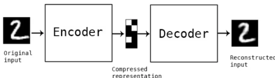
The network consists of two parts, encoder part and decoder part. In figure 2.5, the encoder part encodes the origin data, which is a chart represented by matrix, to a compressed representation. The decoder part uses these representations to reconstruct the input.

Figure 2.5: Encoder and Decoder.

x0 =h(x) (2.8)

r=g(x0) (2.9)

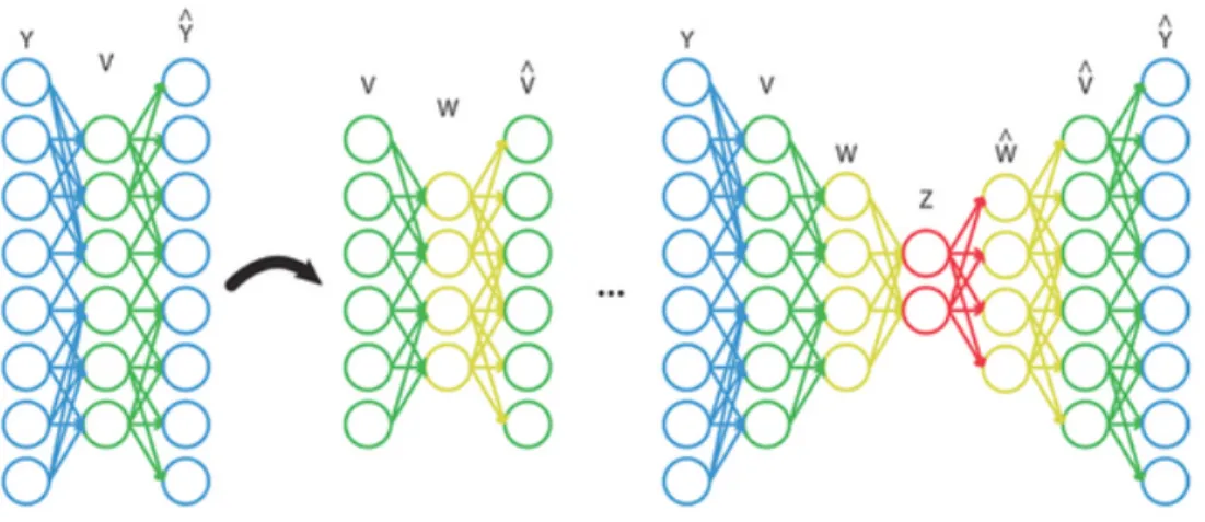
Autoencoder can be stacked in this way but each layer must be trained in advance using Restricted Boltzmann Machine (RBM). Like other neural networks, the gra-dient descent method is used to train the weight values of the parameters. In our experiment, the dimension is reduced to a half of the input size. Autoencoder is

Figure 2.6: Stacked Autoencoder

also trained to minimize reconstruction errors (such as squared errors):

L(x, r) = (||x−r||)2 (2.10)

There are a bunch of variants of Autoencoder, like sparse Autoencoder, Stacking Autoencoder layer by layer, adding noise to input layer to improve the generative ability. Hinton [HS06] proposed to use RBM to pre-train weights for every layer to find an optimal initial weights because the training of neural network is a non-convex optimization process. In our model, we just use 1 layer Undercomplete Autoencoder to train our model. Figure 2.6 shows the stacked Autoencoder1.

1_{source: https://www.researchgate.net/figure/274728436 fig2}

Chapter 3

Improving DKT with More

Features

Intelligent tutoring systems (ITS) often collect numerous features of students work, including information pertaining to problems, instructional aid, and time spent on individual tasks. Data in different levels are collected like school level, teacher level, student level and problem level, skill level and action level. In order to make full use of these additional data, many models and algorithms have been proposed to improve the prediction performance of models. For example, students response time, hint request and number of attempts are added to make better student models [FHK09], hint usage and the number of attempts needed to find the problem answer are adopted to predict the performance in the sequence of actions (SOA) model [DZWH13]; partial credit history acquired based on the number of hints used and the number of attempts are used to predict the probability of students getting the next question correct [VIAWH15].

In this paper, we do something similar using these extra features to improve prediction performance. In our experiment, correctness, students response time,

at-tempt number, and first action are selected for consideration because these features recorded by almost all learning platforms are strongly related to the students’ per-formance. All input information is converted into a sequence of fixed-length input vectors in the RNN model, representing problem-level or skill-level covariates while working through a possible multitude of assignments.

As in traditional DKT model, all features including the cross features are rep-resented as one-hot encoding formate, and then concatenate all of them as inputs. However, this kind of representation of features leads to the rapid increase in input layer dimensions, so Autoencoder algorithm is adapted as dimensional reduction because the naive nature of neural network makes it easy to be embedded to DKT model here.

3.1

Feature engineering

As previously described, it is easy to incorporate useful information such as this into the input layer of a neural network. However, the key consideration is how feature engineering is performed on these features. Feature engineering plays a vital role in representing features effectively. NTU team[YLH+_{10] incorporated a large} number of features and cross-features into a vector-space model and then trained a traditional classifier. They also identified some useful feature combinations to improve the performance. Cross features were used in the original DKT work as well, utilizing a one-hot encoding to represent correct and incorrect responses for each skill separately as a vector of 2 times the number of skills; alternatively, such information could be represented separately, with a one-hot encoding representing skills, and just one binary metric to indicate correctness equating to a vector of the number of skills plus 1. In wide-and-deep learning proposed by Google [CKH+_16],

sparse features and cross features are selected for wide part, while the continuous columns and the embedding dimension for each categorical column are selected for deep part. These exemplary models use the engineering of features to improve model accuracy helping to motivate the methodology of this work.

3.1.1

Cross Features

Cross Features is a method to encode two or more features into one feature to represent the concurrence appearance of these features. Numerical features and cat-egorical features all can be represented using cross features. The following equations show the method to calculate combination of two features. For categorical data, it is represented using one-hot encoding here.

C(et, ct) =et+ (max(E) + 1)∗ct (3.1)

C(ct, et) =ct+ (max(C) + 1)∗et (3.2)

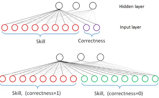
The key reason to use cross features rather than separate features is because separate will degrade the performance of result because weight unbalance in neural network. In figure 3.1, skill features have 8 values, and correctness features is binary. Separate features method needs 8 weights between all skill and one hidden node and 2 weights between correctness and one hidden node. Only 2 weights in separate situation can’t represent the change of whole 8 skills.

3.1.2

One-Hot Encoding

One-hot encoding transforms categorical features to a format that works better with classification and regression algorithms. Take the following student records for example, the SkillID feature involve four values here: S001, S003, S005, S008.

Figure 3.1: weights above: separate features below: cross feature

Student Name Skill Id First Action Time(s) Correctness

Mary S005 hint 100 1

Jack S003 attempt 20 1

Jack S008 attempt 50 0

Abby S001 scaffold 200 0

Alisa S005 attempt 120 1

Table 3.1: Student records example

These values can be encoded to nominal values, but it doesn’t make sense from a machine learning perspective, because we can’t say that S008 is greater than S003. What we do instead is to generate one boolean column for each category and only one of these columns could take on the value 1 for each sample. Hence, the one-hot encoding formate of SkillID feature can be represented in table 3.2.

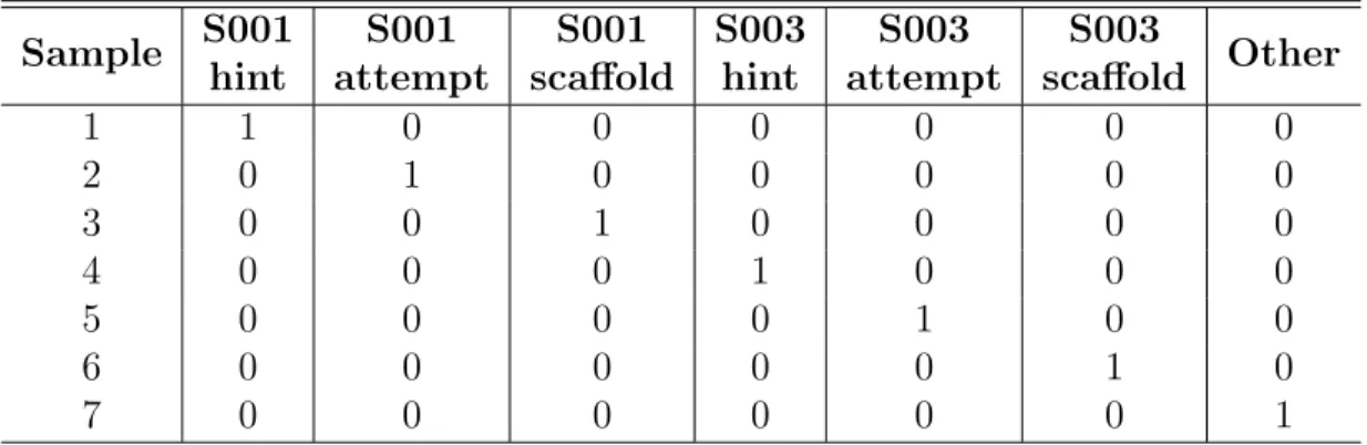
Therefore, the one-hot encoding for the values of two features, Skill ID: S001 or S003 and First Action: hint, attempt, scaffold, can be represented in table 3.3. Since one-hot encoding constructs a pretty sparse matrix with the same number of category type to represent the value of that feature, the shortcoming is obvious

Sample S001 S003 S005 S008

1 1 0 0 0

2 0 1 0 0

3 0 0 1 0

4 0 0 0 1

Table 3.2: One-hot encoding

Sample S001 S001 S001 S003 S003 S003 Other

hint attempt scaffold hint attempt scaffold

1 1 0 0 0 0 0 0 2 0 1 0 0 0 0 0 3 0 0 1 0 0 0 0 4 0 0 0 1 0 0 0 5 0 0 0 0 1 0 0 6 0 0 0 0 0 1 0 7 0 0 0 0 0 0 1

Table 3.3: One-hot encoding of cross features

quickly increased dimension here. Once the category number is too large, the column number will also be large. Two methods can solve such problem, one is reduce dimension, while the other is to represent the category data in other formate like word embedding which is widely used in language model. Here, just one-hot encoding with dimension reduction method is applied.

3.1.3

Word Embedding

Word embedding model1_{, also calledword2vec, is proposed by Mikolov et als [MSC}+_13] to learn vector representations of words. Natural language processing systems treat words as discrete atomic symbols. For example, Porpoise may be represented as Id537 and SeaWorld asId143. These encodings are arbitrary, and provide no useful information to the system regarding the relationships that may exist between the

individual symbols. This means that the model can leverage very little of what it has learned about SeaWorld when it is processing data about Porpoise (such that they are both animals, four-legged, pets, etc.). Representing words as unique, discrete ids furthermore leads to data sparsity, and usually means that we may need more data in order to successfully train statistical models. Using vector representations can overcome some of these obstacles.

Cross Features Feature 1 Feature 2 Feature 3 Feature 4

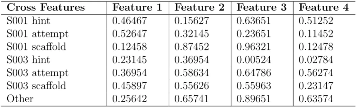
S001 hint 0.46467 0.15627 0.63651 0.51252 S001 attempt 0.52647 0.32145 0.23651 0.11452 S001 scaffold 0.12458 0.87452 0.96321 0.12478 S003 hint 0.23145 0.36954 0.00524 0.02784 S003 attempt 0.36954 0.58634 0.64786 0.56274 S003 scaffold 0.45897 0.55626 0.55963 0.23147 Other 0.25642 0.65741 0.89651 0.63574 Table 3.4: Simulated Word embedding representation of cross features

Table 3.4 uses four embedded features to represent those combination values. It is just a casting relationship between original cross features and compressed four features.

Figure 3.2: Wording Embedding in natural language process

In typically word process scenario, these feature values are initialed randomly and adjusted during training. Since Euclidian distance between two different

sam-ples represent the correlation relationship, it pretty useful for word process. For example, the distance between embedding of word Porpoise and SeaWorld is less than that between embedding of word Paris and Camera in figure 3.22. However, in education data mining, the distance between different samples have no such corre-lation recorre-lationship. That is why one-hot encoding with dimension reduction rather than word embedding method is adopted.

3.1.4

Feature process

The goal of this process in our model, as it pertains to this work and coincides with how input is represented in the DKT model, is to convert the features to categorical data to simplify the input without losing much information. This process is described briefly for each considered feature as follows:

• Exercise tag exhibits differing representations described by either a numeric skill id or the name of the knowledge component in a different dataset. Re-gardless of representation in the data, this is strictly categorical and is handled as such. Exercise tag can be at different levels, such as skill level, problem level and step level. However, too fine level, like step level, is hard to predict because every step owns few training dataset so that it is impossible to be convergent to local optimal weight. In our experiment, we uses skill-level for exercise tag. The balance of exercise number is also critical since exercise with too few training dataset can’t convergent to a local optimized value so that the final performance would be impacted.

• Correctness is represented as a binary value where 1 indicates correctness in the problem and 0 represents an incorrect response. Correctness of current

problem is a key component of input while the correctness of next problem is the label of output layer. However, in each time step, just one label exists because we just know the correctness of current exercise. Some fault values which are neither 0 or 1 may exist in dataset. 0.5 is used as threshold to separate them to binary value.

• Time is a critical feature to reflect student’s understanding of a skill. It is the first response time when the student encountered the exercise. Some ITS platform may record some other time information but just first response time is considered here because it can reflect student’s performance in this exercise. Obviously, it is numerical feature. Two problems exist here if we use the feature as input directly.

1. Numerical features here may cause the model to be too complicated. For example, 101 seconds used in a skill isn’t too much different than 100 seconds. If the time features is used as input features directly, the model has to learn the difference between them.

2. Same time in different exercise represents different students’ performance. For example, skill A is a hard problem, student need more time to con-sider while skill B is relative easy so that less average time is needed. If the time features is used as input features directly, the model can’t consider such difference.

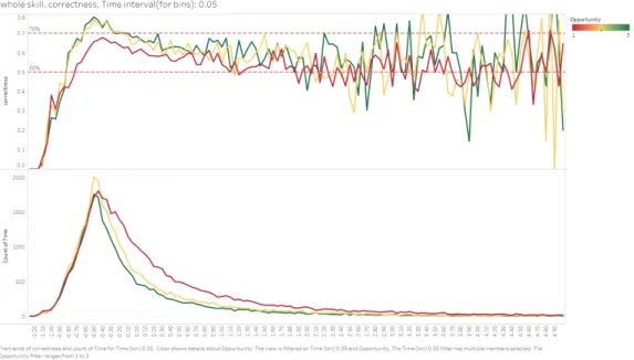
Such relationship exist even in single skill. Three skill are selected in figure 3.4. Opportunity features in ASSISTments 2009 is the number of opportunities the student has to practice on this skill. For different opportunities, the relation-ships between time z-score and correctness still exist.

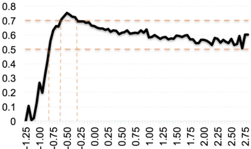
Figure 3.3: Time z-score (X axis) and Correctness (Y axis)

The transformed time feature is z-scored within skill and discretized based on its relationship with correctness as shown in Figure 3.3 which comes from the ASSISTments 2009 datasets. Different skills need different times to fin-ish. In other words, the mean time of finishing different skills are different. Therefore, we transfer the time to the z-score for different skills. The z-score is still numerical, but small differences in z-score don’t represent important differences. Therefore, we discrete the z-score to a categorical feature. In our model, we arbitrarily select 5 categories. In figure 3.3, too little time, like less than −0.75, has obvious worse performance. Meanwhile, the increase of time after a threshold hasn’t much impact on correctness. Therefore, two reference lines of correctness, 50% and 70%, are selected for the discretized boundaries to divide the time to four categories.

• Attempt count is the number of times a student entered an problem. It rep-resents how many times the student has exercised this problem. Obviously, it should be a parabola between attempt count and mastering of this prob-lem. More times less a threshold means more possibility that the student can answer this problem correctly. Sometimes, even more times encountered has

Figure 3.4: Time z-score and correctness for different opportunity

no help in answering this problem correctly since the student give up this chance or lost confidence to answer it. This numerical feature is discretized as [0,1, other] in ASSISTments and [== 1,1 < and <= 5, > 5, other] in Open Learning Initiative as described further in a later section.

• First action is strictly categorical, representing if a student makes an attempt or requests help within the system as a first action. For example, ASSISTments use three value to represent the first action type. 0 represents that student attempts to answer the problem, 1 represents that student uses hint for the problem, and 2 represents that students uses scaffolding help to finish the problem. Different action types can obviously reflect student’s understanding in one exercise (or skill). Attempt means the student have confidence in some degree to answer the problem correctly while asking for help means he or she has no confidence. Interesting, students may have totally different performance after asking for help. He or she may master the skill or this help may provide

Figure 3.5: Time z-score and correctness for single skill no help for understanding the problem.

Different ITS platforms record different features according to the requirement. However, these four features are almost recorded in all platforms. Therefore, just these four features are considered here. Many different process methods can be applied in feature engineering. Just few simple process methods with arbitrary hyper parameters are applied. The hyper parameters can be selected by means of cross-validation.

3.2

Concatenate encoded features

After converting to categorical data, features are represented as a sparse vector using one-hot encoding. Papers [PBH+_{15] [YLH}+_{10] [CKH}+_{16] show that combination} of some input features into cross features as input can improve model accuracy. The cross features of exercise and correctness, as well as time and correctness are selected in our model. The selection of cross features is relatively arbitrary and

cross-validation is a feasible method to find the optimal cross features. All the encoded features, which includes single features and cross features, are concatenated to construct the input vector in figure 3.6. The input vector is constructed by

Figure 3.6: Concatenated encoded features

concatenating one-hot encodings for separate features as illustrated in Figure 3.6, where vt represents the resulting input vector of each student exercise. et refers to the exercise tag, while ct refers to correctness, and tt represents time. C() is the cross feature, O() is the one-hot encoder format, and the _ _{operator is used to} denote concatenation.

[ht]vt =O(C(et, ct))_O(C(tt, ct))_O(tt) (3.3)

An alternative method, word embedding, is also proposed to represent the feature in neural network, particularly in nature language process. In large dataset like word process, every word has enough training dataset so that the weights of neural network can be convergent to be optimal values. Here we just use one-hot encode due to the few number of skill, only 100+. For some other features like problem level id and action, word embedding is an effective encoded method without good effect

because one encoding method may recover to original features but can’t extract the internal feature. For example, word embedding in language process can get the correlation between different words using the euclidean distance but features in education data mining, like problem id, action id and student id, have no such correlation. It just shows the appearance order of problem id and action id so it has no strong support to knowledge tracing prediction.

3.3

Reduce dimension using Autoencoder

Using cross features leads to a rapid increase of the dimensionality of the input vector. RNNs are considerably more computationally expensive due to the compar-atively larger number of parameters. For example, training a LSTM DKT model with 50 skills and 200 hidden nodes, which needs to learn 250,850 parameters, takes 3.5 minutes per epoch, equating to more than 14 hours when using a 5 fold cross validation run over 50 epochs. To this extent, the network structure of DKT may benefit from reduced dimensionality, particularly if this can be achieved without sacrificing performance.

The goal of dimensionality reduction is to compress the signals in size and to discover compact representations of their variability. Two widely used dimen-sionality reduction algorithms are the methods of Principal Component Analysis (PCA) [Jol02] and Multi Dimensional Scaling (MDS) [KW78] for the problem of linear dimensionality reduction and Locally Linear Embedding (LLE) for the prob-lem of nonlinear dimensionality reduction. Both methods are eigenvector methods designed to model linear variabilities. In PCA, the linear projections of greatest vari-ance from the top eigenvectors of the data covarivari-ance matrix are computed. While the low dimensional embedding that best preserves pairwise distances between data

points are computed in MDS. LLE [SR00] is an unsupervised learning algorithm that computes low dimensional, neighborhood preserving embeddings of high di-mensional data. In our experiment, we just consider Autoencoder since it is easy to combine it to RNN. PCA and LLE are also potential algorithms for dimension reduction.

Undercomplete Autoencoder is a multilayer neural network with a small central layer that can convert high dimensional data to low dimensional representative en-codings that can be used to reconstruct the high dimensional input vectors; in this way dimensionality is reduced without the loss of too much important information in figure 3.7. Once trained, the output layer can be removed, and the hidden layer can connect to another network layer. In our model, we use the tanh as active

Figure 3.7: Undercomplete Autoencoder.

function to train the Autoencoder to reduce dimension.

v_t0 =tanh(Wed∗vt+bed) (3.4)

yt =tanh(WedT ∗v

0

Figure 3.8: New DKT LSTM Model without Autoencoder

3.4

DKT Extension Model

Figure 3.8 and figure 3.9 depict the resulting model representation utilizing an En-coder layer to support the added features. Figure 3.8 is the new DKT LSTM model without dimension reduction while the figure 3.9 is for model with dimension re-duction. In figure 3.8, vt represents the Concatenated features, and ht means the hidden layers in t time steps and yt means the label of output layers which is the correctness of next problem. The performance of every skill is predicted but just one is supervised because only one label exists at each time step.

In figure 3.9,v_t0 represents the feature vector extracted by Autoencoder according to equation 3.4. The gray arrows mean that weights between these two layers are held constant so the encoder weights needed to be trained separately in advance. In our model, we have tried to fine-tune these weights with Neural Network, the network is overfitting quickly due to the increased weights.

Figure 3.9: New DKT LSTM Model with Autoencoder

3.5

Optimization

As with other binary classification problems in neural network, the training objective is the negative log likelihood of the observed sequence of student responses under the model. We use the exact same cost function as the traditional DKT model.

L=X

t

l(yTδ(qt+ 1), at+1) (3.6)

This objective was minimized using stochastic gradient descent on minibatches. In order to prevent overfitting, dropout [SHK+_{14] is applied to weights of between}

vt and ht and weights of between ht and yt but not weights ht and ht−1 for no dimensional reduction scenario in figure 3.8. For dimensional reduction scenario in figure 3.9, dropout is applied to weights of between v_t0 and ht and weights of

between ht and yt rather than weights ht and ht−1. Dropout is mainly used for feed forward neural networks but not dedicated for recurrent neural network, so the weights between hidden nodes in different time steps are not considered. The dropout rate, which means the percentage of removed weights, is 0.4. This value is selected arbitrarily based on the scope provided in paper [SHK+_14].

In our experiment, only one LSTM layer with 200 hidden nodes is used. Other hyper parameters like time steps and batch size is selected based on the dataset characters. In table 3.5, it shows these parameter values. The epoch number is 50 for all dataset.

Setting ASSISTments 2009-2010 OLI Statics F2011

TimeStep 1,218 1,500

BatchSize 30 10

Epoch 40 40

Table 3.5: Hyper parameter setting

A model with more than one LSTM hidden layer is tested in our experiment, but the performance is degraded due to doubled parameters which increase the complexity dramatically. Other models like simple RNN and GRU nodes are also tested, simple RNN degrade the performance and GRU hidden nodes has similar test performance with LSTM hidden nodes. Because RNN training process is pretty time consuming particularly using cross-validation, just one LSTM hidden layers is considered in our experiment.

Chapter 4

Datasets and Environment

4.1

Datasets

Two educational datasets from ASSISTments and Open Learning Initiative (OLI) are tested in our experiments. These two ITSs are computer-based learning plat-forms which embed practice and assessment throughout the learning process.

The original DKT model with inputs that include only exercise tag and correct-ness is used as a model for comparison. Since it is a time-series algorithm, students whose records are less than 2 are not considered.

Setting ASSISTments 2009-2010 OLI Statics F2011

Student 3,866 332

Skill 124 82

Record 303k 257k

4.1.1

ASSISTments 2009-2010

ASSISTments, founded by Professor Neil T. Heffernan in Worcester Polytechnic Institute (WPI), is a computer-based learning system that simultaneously teaches and assesses students outside class. This dataset was gathered from ASSISTments skill builder problem sets 1, which are assignments in which a student works on similar questions until he or she can correctly answer n consecutive problems cor-rectly (where n is usually 3). After completion, students do not commonly rework the same skill. This dataset is the benchmark dataset for education data mining research because it is the largest number of open student learning records collected from online learning platform so far.

In the original data version, Xiong et al. [XZVB16] discovered three issues: du-plicated records, mixing main problems with scaffolding problems and repeated re-sponse sequences with different skill tagging (duplication by skill tag). These issues have unintentionally inflated the performance of DKT in the original version, so the updated version of this dataset is adopted here.

Unlike other datasets, the records of a student may not be consecutive be-cause student may answer questions in different days. That is why some previous works [PBH+_{15] reports 15,391 students while others [XZVB16] reports 4,217} stu-dents. There are two methods to process these records. The dataset can be used directly so that the records answered in different days are considered as different stu-dent’s records, whereas all records belong to one student are concatenated because these records represent the performance of same student. In our model, we use the second method to process data. The exercise tag is defined as the skill id. Table 4.1 shows the key statistical information about this dataset, the students number is

1

3,866 and the skill number is 124 and records number is more than 303,000.

4.1.2

OLI Statics F2011

The Open Learning Initiative (OLI) is a computer learning system at Carnegie Mel-lon University to offer online courses to students at school2. OLI embeds assessment into instructional activity and collect real-time data of student-use in those activities with the students permission.

This dataset3 _{was from a college-level engineering statics course in OLI. It} pro-vide dataset from different semesters. Fall 2011 is adopted here because it involves 332 students. Unlike ASSISTments dataset whose skill ID is a number, this dataset use text description to represent skill ID. The text is covert to category data type.

Since it is a time-series algorithm, students whose records contain less than 2 time steps are not considered. Table 4.1 shows the key statistical information, it involves 332 students, 82 skills and more than 257,000 records totally.

4.2

Evaluation Metrics

As in paper [XZVB16], the accuracy was evaluated using Area Under Curve (AU C) and the square of Pearson correlation (r2_{). AU C and r}2 _{provide robust metrics} for evaluation predictions where the value being predicted is either a 0 or 1 also represents different information on modeling performance. An AU C of 0.50 always represents the scored achievable by random chance and a higher AU C score rep-resents higher accuracy. r2 is the square of Pearson correlation coefficient between the observed and predicted values of dependent variable. In the case of r2, it is normalized relative to the variance in the data set and it is not directly a measure

2_{source: https://oli.cmu.edu/get-to-know-oli/learn-more-about-oli/} 3_{https://pslcdatashop.web.cmu.edu/Project?id=48}

of how good the modeled values are, but rather a way of measuring the proportion of variance we can explain using one or more variables. r2 is similar to root mean squared error (RM SE) but is more interpretable. For example, it is unclear whether a RMSE of 0.3 is good or bad without knowing more about the dataset. However, a r2 _{of 0.8 indicates the model accounts for most of the variability in the data set.}

NeitherAU Cnorr2 _{method is a perfect evaluation metric, but their combination} accounts for different aspects of a model and provides us a basis to evaluate our models.

4.3

Running Environment

For replicability, the running environment is reported as the following: • Hardware: i5600 processor, 16G RAM, GTX 1070 (8G) graphics cards

• OS: Ubuntu 14.04 64-bit. Ubuntu 16.04, the latest version, is not compatible with Tensorflow GPU version.

• Package: Tensorflow 0.10 Linux GPU version.

• Python version: 3.4. (python version 3.5 is not compatible with Tensorflow GPU version)

• NVIDIA CUDA version: 7.5 • NVIDIA cuDNN version: 4.0

• Other package: Pandas, Numpy, Keras (statistic parameter number)

Chapter 5

Results

5-fold student level cross validation is applied to reduce the variance of test result which is evaluated by AU C and (r2_{). Many possible feature combinations exist,} but only a selected few are explored here. In table 5.1 and 5.2, S means skill id, C means correctness, T means time, ACT means first action, AT T means attempt number,_ _{means concatenation.}

Model Autoencoder AU C(%) r2 Baseline: S/C No 83.1±0.6 0.324±0.012 S/C _ _{T/C No 85.8±0.7 0.391±0.015} S/C _ T/C Yes 86.7±0.4 0.410±0.008 S/C _ _T/C _ _T __A CT _ AT T No 86.1±0.4 0.398±0.011 S/C _ T/C _ T _ACT _ AT T Yes 86.7±0.2 0.411±0.005 S/C _ _T/C _ _T/S _ _T __A CT _ AT T Yes 86.7±0.5 0.412±0.012 Table 5.1: ASSISTments 2009 dataset Result

On both datasets in table 5.1 and 5.2, models with incorporated features in which Autoencoder isn’t used outperform the baseline, the original DKT model. In the ASSISTments 2009 dataset, AU C value is improved to 85.8 from 83.1 and r2 _value increases to 0.391 from 0.342 after adding the cross feature of skill and correctness. In the Statics 2011 dataset, the AU C value increases to 73.1 from 70.6 andr2 _value

Model Autoencoder AU C(%) r2 Baseline: S/C No 70.6±0.7 0.105±0.009 S/C _ _{T/C No 73.1±0.5 0.135±0.010} S/C _ T/C Yes 73.5±0.9 0.142±0.012 S/C _ _T/C _ _T __A CT _ AT T No 73.2±0.5 0.140±0.011 S/C _ T/C _ T _ACT _ AT T Yes 74.0±0.5 0.148±0.009 S/C _ _T/C _ _T/S _ _T __A CT _ AT T Yes 74.0±0.9 0.147±0.016 Table 5.2: OLI Static 2011 dataset Result

is from 0.105 to 0.135 if only add cross feature of skill and correctness. Actually, if only incorporating cross feature of skill and correctness, the dimension of input layer only increases 8,4(time)∗2(correctness) so that it almost has same running efficiency as original DKT model. However, it exhibits only a marginal increase to this upon adding time, first action, and attempt count into the input vectors. It is easy to understanding result, because linear dependence exist between these features.

The adoption of Autoencoder when compared to models using the same features also shows increased performance, supporting its usage for reducing dimensionality. The compressed dimension is half of the input layer. In the ASSISTments 2009 dataset,AU C value is improved to 86.7 from 85.8 andr2 _{value increases from 0.391} to 0.410. While in OLI Statics dataset, AU C value is from 73.1 to 73.5 while r2 value is from 0.135 to 0.142. In our analyses, the model incorporating all features in the last record in table 5.1 and 5.2 was not even feasible without the use of this Autoencoder, deeming it necessary to use when given large dimensional inputs. The different number of hidden node can impact the result, we tried 1/4 of the original input dimension, the performance of test result degrade a little bit but not increase. In summary, the incorporation of more features into DKT can improve the pre-diction accuracy, and the Autoencoder method can effective reduce the resource

need for training without similar prediction accuracy if the hidden nodes number is selected properly.

Chapter 6

Discussion

6.1

Drawback in constructing skill graph

Paper [PBH+15] proposes to use DKT model to get the skill graph or get the best exercise path which can improve the whole performance in study because DKT model can predict the performance of student in every exercise based on previous exercises. However, from skill transfer perspective, the model is trained according to a relative fixed skill transfer pattern. 30 skills are randomly selected from both datasets to construct the skill transfer chart in figure 6.1. Take ASSISTments 2009 dataset for example, skill 9 mainly transfer to skill 8, and skill 10 mainly transfer to skill 9 in figure 6.1. Therefore, it is unconvinced to infer student’s performance in skill 14 based on skill 10 because there is no training data from skill 10 to skill 14. However, we can use DKT model to predict the NPC because the test dataset and validation test dataset follow the same transfer pattern as training dataset.

6.2

Future work

Figure 6.1: ASSISTments Dataset skill transfer

• Explore even more student features [GZM11] like class-level features and school-level features and explore more features engineer method in different manners, such as tokening the words of knowledge components for different exercise rep-resentations. Cross-validation is a effective way to select features.

• Explore the wide and deep approach [YLH+10] in how the features are repre-sented within model training to combine the advantage of memorization and generalization. Memorization means the frequent co-occurrence of features and exploit the correlation in historical data, while the generalization is based on transitivity of correlation and explore new feature combination. Memorization

of feature is represented by a wide set of cross-product feature transformations and generalization use more feature engineering effort to single features. • Explore different dimensionality reduction methods like linear transformation

like Principal Component Analysis (PCA), Multi Dimensional Scaling (MDS) and non-linear methods like Locally Linear Embedding (LLE) and other Au-toencoder methods. Many variants of AuAu-toencoder can be used to strength the ability, like adding noise to the input layer, add different regularization to the cost function, stacking deep layers in encoder and decoder part or use RBM to optimize the initial weights.

• Explore DKT model to solve other prediction problems in education data mining. NPC is just a kind of label for knowledge tracing. Some other new prediction model are also available such as wheel spinning [BG13], student dropout, or hint usage.

• Explore the multi-task prediction to improve the prediction accuracy. For ex-ample, because wheel spinning and NPC are strongly related, adding Wheel spinning label to output layer to train the weights may improve the perfor-mance of NPC. However, it is necessary to pay attention to the missing labels in such dataset. NPC almost can guarantee that every prediction problem have label but other may not. Many labels are generated according to differ-ent standards. Take affect label for example, the labels like bored, concdiffer-entrat- concentrat-ing, confused and frustrated, are generated every 20 seconds during student’s answering question process.

Bibliography

[Atk72] Richard C Atkinson. Optimizing the learning of a second-language vocabulary. Journal of Experimental Psychology, 96(1):124, 1972. [BCMC08] Joseph E Beck, Kai-min Chang, Jack Mostow, and Albert Corbett.

Does help help? introducing the bayesian evaluation and assessment methodology. In International Conference on Intelligent Tutoring Sys-tems, pages 383–394. Springer, 2008.

[BG13] J. E. Beck and Y. Gong. Wheel-spinning: Students who fail to master a skill. InInternational Conference on Artificial Intelligence in Educa-tion, pages 431–440. Springer, 2013.

[CA94] A. T. Corbett and J. R. Anderson. Knowledge tracing: Modeling the acquisition of procedural knowledge. User Modeling and User-Adapted Interaction, 4(4):253–278, 1994.

[CKH+16] Heng-Tze Cheng, Levent Koc, Jeremiah Harmsen, Tal Shaked, Tushar Chandra, Hrishi Aradhye, Glen Anderson, Greg Corrado, Wei Chai, Mustafa Ispir, et al. Wide & deep learning for recommender systems. InProceedings of the 1st Workshop on Deep Learning for Recommender Systems, pages 7–10. ACM, 2016.

[dBCA08] Ryan SJ d Baker, Albert T Corbett, and Vincent Aleven. More accu-rate student modeling through contextual estimation of slip and guess probabilities in bayesian knowledge tracing. In International Confer-ence on Intelligent Tutoring Systems, pages 406–415. Springer, 2008. [DZWH13] Hien Duong, Linglong Zhu, Yutao Wang, and Neil Heffernan. A

pre-diction model that uses the sequence of attempts and hints to better predict knowledge:” better to attempt the problem first, rather than ask for a hint”. In Educational Data Mining 2013, 2013.

[ES02] Douglas Eck and J¨urgen Schmidhuber. Learning the long-term struc-ture of the blues. In International Conference on Artificial Neural Networks, pages 284–289. Springer, 2002.

[FHK09] M. Feng, N.T. Heffernan, and K. R. Koedinger. Addressing the assess-ment challenge with an online system that tutors as it assesses. User Modeling and User-Adapted Interaction, 19(3):243–266, 2009.

[GS05] Alex Graves and J¨urgen Schmidhuber. Framewise phoneme classifi-cation with bidirectional lstm and other neural network architectures. Neural Networks, 18(5):602–610, 2005.

[GSS02] Felix A Gers, Nicol N Schraudolph, and J¨urgen Schmidhuber. Learn-ing precise timLearn-ing with lstm recurrent networks. Journal of machine learning research, 3(Aug):115–143, 2002.

[GZM11] L Gunter, J Zhu, and SA Murphy. Variable selection for qualitative interactions. Statistical methodology, 8(1):42–55, 2011.

[HS97] Sepp Hochreiter and J¨urgen Schmidhuber. Long short-term memory. Neural computation, 9(8):1735–1780, 1997.

[HS06] G. E. Hinton and R. R. Salakhutdinov. Reducing the dimensionality of data with neural networks. Science, 313(5786):504–507, 2006. [JCK09] P.I. PAVLIK JRa, H. Cen, and K. R. Koedinger. Performance factors

analysis–a new alternative to knowledge tracing. Online Submission, 2009.

[Jol02] Ian Jolliffe. Principal component analysis. Wiley Online Library, 2002. [KLM16] Mohammad Khajah, Robert V Lindsey, and Michael C Mozer. How

deep is knowledge tracing? arXiv preprint arXiv:1604.02416, 2016. [KTS+_{14] Andrej Karpathy, George Toderici, Sanketh Shetty, Thomas Leung,}

Rahul Sukthankar, and Li Fei-Fei. Large-scale video classification with convolutional neural networks. In Proceedings of the IEEE conference on Computer Vision and Pattern Recognition, pages 1725–1732, 2014. [KW78] Joseph B Kruskal and Myron Wish. Multidimensional scaling,

vol-ume 11. Sage, 1978.

[KWLM14] Mohammad Khajah, Rowan Wing, Robert Lindsey, and Michael Mozer. Integrating latent-factor and knowledge-tracing models to pre-dict individual differences in learning. In Educational Data Mining 2014, 2014.

[LBD+_{89] Yann LeCun, Bernhard Boser, John S Denker, Donnie Henderson,} Richard E Howard, Wayne Hubbard, and Lawrence D Jackel. Back-propagation applied to handwritten zip code recognition. Neural com-putation, 1(4):541–551, 1989.

[MSC+13] Tomas Mikolov, Ilya Sutskever, Kai Chen, Greg S Corrado, and Jeff Dean. Distributed representations of words and phrases and their com-positionality. In Advances in neural information processing systems, pages 3111–3119, 2013.

[Ola15] Christopher Olah. Understanding LSTM Networks. http://colah.github.io/posts/2015-08-Understanding-LSTMs/, 2015. [Online; accessed 27-March-2017].

[PBH+_{15] C. Piech, J. Bassen, J. Huang, M. Sahami S. Ganguli, L. Guibas, and} J. Sohl-Dickstein. Deep knowledge tracing. In Advances in Neural Information Processing Systems, pages 505–513, 2015.

[PH10] Zachary A Pardos and Neil T Heffernan. Modeling individualization in a bayesian networks implementation of knowledge tracing. In Interna-tional Conference on User Modeling, Adaptation, and Personalization, pages 255–266. Springer, 2010.

[SHK+_{14] Nitish Srivastava, Geoffrey E Hinton, Alex Krizhevsky, Ilya Sutskever,} and Ruslan Salakhutdinov. Dropout: a simple way to prevent neu-ral networks from overfitting. Journal of Machine Learning Research, 15(1):1929–1958, 2014.

[SLJ+15] Christian Szegedy, Wei Liu, Yangqing Jia, Pierre Sermanet, Scott Reed, Dragomir Anguelov, Dumitru Erhan, Vincent Vanhoucke, and Andrew Rabinovich. Going deeper with convolutions. In Proceedings of the IEEE Conference on Computer Vision and Pattern Recognition, pages 1–9, 2015.

[SR00] Lawrence K Saul and Sam T Roweis. An introduction to locally linear embedding. unpublished. Available at: http://www. cs. toronto. edu/˜ roweis/lle/publications. html, 2000.

[SWG05] J¨urgen Schmidhuber, Daan Wierstra, and Faustino Gomez. Evolino: Hybrid neuroevolution/optimal linear search for sequence learning. In Proceedings of the 19th international joint conference on Artificial in-telligence, pages 853–858. Morgan Kaufmann Publishers Inc., 2005. [VIAWH15] Eric G Van Inwegen, Seth A Adjei, Yan Wang, and Neil T Heffernan.

Using partial credit and response history to model user knowledge. International Educational Data Mining Society, 2015.

[WHB10] Yutao Wang, Neil T Heffernan, and Joseph E Beck. Representing stu-dent performance with partial credit. InEducational Data Mining 2010, 2010.

[WKHE16] Kevin H Wilson, Yan Karklin, Bojian Han, and Chaitanya Ekanad-ham. Back to the basics: Bayesian extensions of irt outperform neural networks for proficiency estimation. arXiv preprint arXiv:1604.02336, 2016.

[XZVB16] X. Xiong, S. Zhao, E.G. VanInwege, and J. E. Beck. Going deeper with deep knowledge tracing. In Proceedings of the 9th International Conference on Educational Data Mining (EDM 2016), pages 545–550, 2016.

[YLH+_{10] Hsiang-Fu Yu, Hung-Yi Lo, Hsun-Ping Hsieh, Jing-Kai Lou, Todd G} McKenzie, Jung-Wei Chou, Po-Han Chung, Chia-Hua Ho, Chun-Fu Chang, Yin-Hsuan Wei, et al. Feature engineering and classifier en-semble for kdd cup 2010. In KDD Cup, 2010.