Spreadsheet smells

(1)

Hugo Manuel Sousa Ribeiro Spreadsheet Smells

Tese de Mestrado

Mestrado em Informática

Trabalho efectuado sob a orientação de Prof. Dr. João Saraiva e Dr. Jácome Cunha

(2)

(3)

acknowledgements

This dissertation has been influenced by many people, some over the past year, and some over my entire life. I am specially thankful to my supervisors Ph.D João Saraiva and Ph.D Jacome Cunha for their amazing skill in matter of guidance, they always knew how to put me in the right track.

Then, I must thank my parents and my brother for all the patience, support, and all the teachings given. They made me who I am today, as a student and a human being.

I mus thank my girlfriend Rita Barros for all the support, patience to put up with my bad mood, and willing to listen when I felt more below. She was the best!

I cannot forget my friends, specially Nhoca, Lautas and Paulo Lopes they had an impor-tant role helping me to relax, keep the cool, make company and gave their support when I needed.

I must also thank Software Improvement Group in general, José Pedro, Miguel Ferreira and Joost Visser for the time spent, hospitality and knowledge provided during my stay at their headquarters.

To all the personal that worked close to me during this past year, specially Christophe Peixoto, André Riboira, Jorge Mendes and others, that helped me when some problem showed and I tried the answer with them. And to all the people that I didn’t mention but here and there helped me to go through this past year.

(4)

(5)

Resumo

Olhando para as folhas de cálculo como uma linguagem de programação faz dela a lin-guagem mais usada em todo mundo. Na verdade alguns estudos dizem que os chamados de programadores não-profissionais excedem em grande número os programadores profis-sionais. Por causa disso e da falta de mecanismos como abstracção, encapsulamento, ou programação estruturada, 90% das folhas de cálculo têm erros. Esta dissertação apresenta um esforço feito para ajudar com este problema.

O objectivo principal desta dissertação é desenvolver uma ferramenta que permita de-tectar possiveis problemas em folhas de cálculo, esses problemas chamamos "smells" (uma indicação superficial que geralmente aponta para um problema mais profundo). Para isso, introduzimos alguns conceitos teoricos como metricas e smells, como por exemplo o Smell das Dependências Funcionais que adaptamos das bases de dados. Apresentámos o estudo que foi feito, mostrando os resultados obtidos pela ferramenta aplicada a um grande con-junto de folhas de cálculo, o EUSES Corpus.

(6)

(7)

Abstract

Viewing spreadsheets as a programing language makes it the most used programming language worldwide. In fact some studies performed show that the so called "end-user" programmers surpass the professional programmers by far. Because of this and the lack of support for abstraction, testing, encapsulation or structured programming, 90% of the spreadsheets in the real world have errors. This dissertation presents an effort to help with this problem.

The main goal of this dissertation is to create a technique that allows us to detect prob-able problems in spreadsheets, problems called smells (a surface indication that usually corresponds to a deeper problem). Thus, we first introduce some theoretic concepts like metrics and smells, such as for instance the Functional Dependency Smell that was adapted from databases. We present the study we made, showing the results obtained with the tool applied to a large set of spreadsheets, the EUSES corpus.

(8)

(9)

List of Figures

1.1 Example of a spreadsheet. . . 2

2.1 Spreadsheet error taxonomy. . . 7

3.1 Different metrics for different stages. . . 12

3.2 The Software Quality Model ISO/IEC 9126. . . 13

4.1 Motivation example for smells . . . 19

4.2 Window of search in Type Smells . . . 21

4.3 Window of search in Type Smells . . . 22

4.4 Reference to Blank Cells Example . . . 24

4.5 Attribute match lattice . . . 26

4.6 Conditional Functional Dependency Example . . . 27

4.7 Ochiai Example . . . 28

4.8 Output of ochiai to the spreadsheet in Figure 4.7 . . . 29

5.1 “SmellSheet Detective”Architecture. . . 33

5.2 Horizontal Organization Data Example. . . 35

5.3 Vertical Organization Data Example. . . 35

6.1 Formula Relative Explanation. . . 69

(14)

(15)

List of Tables

4.1 Mantyla Taxonomy . . . 18

4.2 Functional Dependency Example 1. . . 25

4.3 Functional Dependency Example 2. . . 25

5.1 Data orientation in spreadsheets. . . 32

5.2 DB_basicdata HAFO Permits. . . 36

5.3 DB_cattrainchecklist Sheet1. . . 36

5.4 DB_duck94_otherdata RHBSept. . . 36

5.5 DB_SteamTool 3. STEAM SYSTEM PROFILING. . . 37

5.6 DB_NamingConventionDataS#A855B Summary. . . 37

5.7 DB_rmomatrix MATRIX. . . 37

5.8 DB_ADC%20Databases ADC_data_Table1. . . 37

5.9 DB_Population Pop.l1. . . 38

5.10 DB_dab1 Sheet3. . . 38

5.11 Database Result Totals. . . 39

5.12 Database Statistical Result by Smell. . . 39

5.13 Database Statistical Result by Level. . . 40

5.14 FIN_CMSAauditreport2002_2003 Sheet1. . . 41

5.15 FIN_FinalAnnexFSSN06001 Annex3. . . 41

5.16 FIN_Cost%20Statement Blad1 (2). . . 41

5.17 FIN_Financial%20Compariso#A7ED8 Financial Comparison Analysis. . . 42 xiii

(16)

xiv LIST OF TABLES

5.18 FIN_finrpt00 Five Year Review. . . 42

5.19 FIN_income-statement Income Statement. . . 42

5.20 FIN_MATHCOUNTS%20Financial Sheet1. . . 42

5.21 FIN_hospitaldataset2002 MEMORIAL. . . 42

5.22 Financial Result Totals. . . 43

5.23 Financial Statistical Result by Smell. . . 44

5.24 Financial Statistical Result by Level. . . 44

5.25 GRD_483_grades_web grades. . . 45

5.26 GRD_as474gradestopost lab grades. . . 45

5.27 GRD_2003FP785DZ 2003FP785DZ. . . 46

5.28 GRD_dss-2001 Sheet1. . . 46

5.29 GRD_firsttrimester Sheet1. . . 46

5.30 GRD_99execgrades Exec Grades. . . 46

5.31 GRD_CRJ%20230_Spring%20grades ClassRosterExportServlet. . . 47

5.32 GRD_anat1f03post post1. . . 47

5.33 GRD_2000_places_School Sheet1. . . 47

5.34 Grades Result Totals. . . 48

5.35 Grades Statistical Result by Smell. . . 48

5.36 Grades Statistical Result by Level. . . 49

5.37 HOME_finalGRADES Writing Assng. . . 50

5.38 HOME_AClassSchedule2003 Schedule. . . 50 5.39 HOME_D6 D6.2. . . 50 5.40 HOME_comments02 Sheet2. . . 51 5.41 HOME_2101_Homework 2101. . . 51 5.42 HOME_cgs1540 Sheet1. . . 51 5.43 HOME_Econ%20homework%20one Sheet1. . . 51 5.44 HOME_Fin_Eval-Budgets-Web 1997. . . 51 5.45 HOME_cis105Winter2004calendar January 2004. . . 52

(17)

LIST OF TABLES xv

5.46 Homework Result Totals. . . 52

5.47 Homework Statistical Result by Smell. . . 53

5.48 Homework Statistical Result by Level. . . 53

5.49 INV_1996El_Final_Files WRAP Domain. . . 54

5.50 INV_Inventory%20Log%20Sheet Basement. . . 54

5.51 INV_AssetAccountCodes ACCT Asset. . . 54

5.52 INV_outline TOC for Pam. . . 54

5.53 INV_InsuranceApplication-#A8A10 Page 4. . . 55

5.54 INV_Licensing%20Inventory#A88C0 Purchase Data. . . 55

5.55 INV_PrimaryProduction2003 Dec. . . 55

5.56 INV_ICATINV iccat tag. . . 55

5.57 INV_2003-fairact II. Inherently Governmental. . . 56

5.58 INV_CL2003-007_AnnexB ANNEX B. . . 56

5.59 Inventory Result Totals. . . 57

5.60 Inventory Statistical Result by Smell. . . 57

5.61 Inventory Statistical Result by Level. . . 57

5.62 MOD_skill-certificates-071103 West. . . 58

5.63 MOD_Analytic_work Sheet 1. . . 59

5.64 MOD_rs2002-0152att CALFED Watershed. . . 59

5.65 MOD_PSCCUNYawards Sheet1. . . 59

5.66 MOD_IROS2003-Program-Final Sessions. . . 59

5.67 MOD_Teaching%20Evaluation#A8732 Sheet1. . . 59

5.68 MOD_CancelsFullstOct02 CancelsFullLstOct02. . . 60

5.69 Modeling Result Totals. . . 60

5.70 Modeling Statistical Result Totals by Smell. . . 61

5.71 Modeling Statistical Result Totals by Level. . . 61

5.72 Global Result Totals. . . 62

(18)

xvi LIST OF TABLES A.1 Cell Level Metrics. . . 71 A.2 Sheet Level Metrics. . . 72 A.3 Spreadsheet Level Metrics. . . 72

(19)

Chapter 1 Introduction

The spreadsheets are used worldwide by all kind of person, specially non-professional programmers, the also called "end-user" programmers [22]. An end-user can be a teacher, an engineer, a student, anyone that is not a professional programmer is considered one. These end-user programmers outnumber the professional programmers by far. In fact a study performed by Scaffidiet al. in 2005 estimates that only in U.S. exists 11 million of end users against only 2.75 million of professional programmers [31]. Still in this study they project to 2012 a total of 90 millions of end users from which 55 million will be from spreadsheets or databases.

The dimension of users presented by Scaffidi implies that millions of new spreadsheets are created every year. And because these end users are not professional programmers when they create a new spreadsheet they usually do not look to any principles of programming, instead all they care is getting the job done. This approach by the users, and the lack support for abstraction, testing, encapsulation, or structured programming in spreadsheets as a programming language, leads to the results presented in some studies that report that up to 90% of real-world spreadsheets contain errors [30].

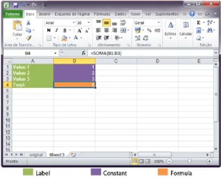
A spreadsheet is a computer adaptation of a paper ledger sheet and it consists of a grid of rows and columns. It is an environment that simplifies manipulation of numbers. A spreadsheet is a digital document composed by a grid of rows and columns filled with cells containing three types of data, Labels, Constantsand Formulas. Labels are text en-tries mainly used to identify items and help understanding the spreadsheet. Constants are numeric, dates or booleans entries that can be used in computation; Formulas are the en-tries that have an equation inside (formula) that will be used to display the resulting value.

(20)

2 CHAPTER 1. INTRODUCTION Formulas must start with "=" symbol and constant values can be used as parameters. For instance a formula can be used to sum all values from a row or column. Formulas can also be just a reference to other cells. By doing this the cell with that formula will present the same value presented in the referenced cell.

Figure 1.1:Example of a spreadsheet.

In spreadsheets the mapping to the cells is made by using a combination of letters (columns) and numbers (rows) for example: the code "A10" represents the first column row 10. In Fig. 1.1 we can see an example of a spreadsheet. The values in the column A (green values1) are Labels, the values in purple are constants (numbers) that will be used by the formula in the cell B4 (orange) to calculate their sum.

Nowadays we can find many software to work with spreadsheets, from the most com-mon solutions desktop-based asExcel [5] or the open source versions of it, thecalcfrom

LibreOffice[9] or fromOpenOffice[10], to the more recent approach brought byGooglea web-based system likeGoogle Docs[13]. This new branch of spreadsheets is just a conse-quence of the evolution of the technology that is rapidly advancing to full web systems.

Many studies refer the high rate of errors in spreadsheets and how this is costly to companies. Thus, in this work we look for smells in spreadsheets so we can lead to the way of improving those spreadsheets. Smells were introduced to the software engineering

(21)

1.1. STRUCTURE OF THE DISSERTATION 3 by Martin Fowler [11] in 1999 and the name points directly to the concept: something that smells is something that does not look correct. This concept has been studied in parallel by us and by Hermmans in [7], but in different perspectives, we do not trace a parallelism between our smells and the ones introduced by Fowler.

In order to detect something that does not look correct in spreadsheets we analyze a large repository of spreadsheets; the EUSES corpus. We used the EUSES Corpus [17] since it contains more than 5000 spreadsheets. The study that we will present is a massive analyze to a randomly selected sample from the EUSES. First we selected a bunch of spreadsheets from each category of the EUSES, and then from those we selected ten sheets from each category, all the picks were random.

1.1 Structure of the dissertation

This dissertation is structured as follows:

Chapter 2: discusses the state of the art and is where we will present some previous studies done by other authors.

Chapter 3: explains the need of measuring software and some guidelines of how should we do it. This chapter also introduces the concept of metric and introduce the metrics that can be used in spreadsheets.

Chapter 4: presents the concept of software smell and how we use it in spreadsheets. In this chapter we describe in detail the smells that we will be using in the “SmellSheet Detective”.

Chapter 5: is where all the evolution results will be shown. This chapter is where we present the studyper se, we describe the sample used, explain the process, present the tool and the results obtained.

Chapter 6: is where we take all the conclusions of the work, and point out some interesting future work.

(22)

(23)

Chapter 2 State of the Art

Summary:

In this chapter we present some of the research that is related to ours. We present works about the measurements of softwares in general, spreadsheet analysis and spreadsheet errors and also present some work in the field of smells, on software and spreadsheets.

Efforts related to our research include a wide range of studies. From studies about spreadsheets errors, spreadsheet analysis, spreadsheet visualization and smells in spread-sheets, to general analysis of software or metric definitions. In this chapter, we will do a brief exposition about those studies.

Measurements:

The main purpose of Alves et al. [2] is to give meaning to values obtained by the use of metrics in measuring software. They present a way to define relevant thresholds so that the results obtained may be better understandable and more meaningful. Alveset al. work rests in three assumptions: “i) it should respect the statistical properties of the metric, such as scale and distribution; ii) it should be based on data analysis from a representative set of systems (benchmark); iii) it should be repeatable, transparent and straightforward to execute.”

Still in the field of measurements we can underline the work made by Heitlager et al. [15]. In this paper, it is presented a way to measure the maintainability of a software that is based on the standard ISO 9126 [18]. This model is not just theoretical, they really

(24)

6 CHAPTER 2. STATE OF THE ART use it in the analysis made by their company "Software Improvement Group".

Spreadsheet Analysis:

Related to spreadsheet analysis we must stress the work of Bergar [3] who presents a list of complexity metrics to be used in spreadsheets. This work does not provide any justification for the metrics chosen. Hodnigget al.[16] defend that the comprehension of a spreadsheet may be simplified by a good technique of visualization, so they use complexity measures as an indicator of a proper visualization. They divide their metrics in three groups: general metrics, where they consider the number of formulas or the number of non-empty cells;

formula complexity, where they include metrics such as the chain calculation or the Fan-in and Fan-out of a cell; and finally the metrics they callfurther complexity argumentswhere they measure the existence of any scripts,e.g.VBA or python, the existence of user-defined functions or external sources.

Smells:

Fowler [11] was the first to introduce the concept of smell and to create a list of 22 smells pointing a possible solution for each one of them. In the sequence of Fowler study, Mantyla et al.[21] has created a taxonomy for the smells listed by Fowler so they could be easier to understand. They created five groups of smells, the bloaters, the object-oriented abusers, the change preventers, the dispensables and the couplers.

Still in smells but now to spreadsheets we should refer the very recent work of Hermans et al. [7] that used smells to detect weaknesses in spreadsheets. They also make a relation between their smells for spreadsheets with those that Fowler listed, presenting, like Fowler did, a possible way of refactoring. Their work differs from the work we present in this thesis in the fundamental approach to define spreadsheet smells: while Hermans adapt Fowler smells to the spreadsheet realm, we analyze a large corpus and based on that we define spreadsheet specific smells.

Spreadsheet Errors:

In this specific field, we refer Powellet al.[26], [27] studies, where they dissects errors in spreadsheets, which type of errors occur, their consequences, which ones are more com-mon, how to prevent them and how to detect them.

(25)

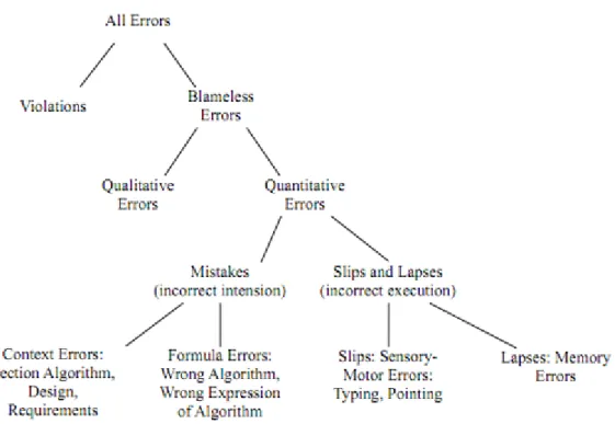
7 More recently by Panko et al.[23] proposed a taxonomy for spreadsheet errors to help other researchers. This taxonomy is a revision of one previously proposed by him [24]. In Figure. 2.1 we can see the new proposed taxonomy.

(26)

(27)

Chapter 3 Software Quality Assessment Based on

Metrics

Summary:

In this chapter we start by introducing the need of measure things daily and then we try to explain why are these measurements needed in the com-puter science, and how they may be done. Finally we talk about metrics for spreadsheets, where we present five groups of metrics and also some metrics that can be used to measure things in spreadsheets. These metrics are grouped by levels: cell, sheet and spreadsheet.

“ Measurements: is the process by which numbers or symbols are assigned to attributes of entities in the real world in such a way as to describe them according to clearly define rules” Fentonet al.[8]

In our daily life we use measurements in almost every task that we accomplish even without realizing it. In the morning when we wake up we measure the time needed to get to work in time, we measure the time needed to warm up the coffee so it do not get to hot or to cold, if we need to pay something in a shop we measure the correct change so we do not get deceived, and in many other tasks. Measurements are built-in our everyday and we need them to understand it and properly interact with it.

In computer science this reality is transposed to our work and we use it for instance to measure the quality of software. Software quality measurement is the quantification to what extent a system possesses the desirable characteristics. This can be made through

(28)

10 CHAPTER 3. SOFTWARE QUALITY ASSESSMENT BASED ON METRICS qualitative or quantitative measures, either way a measurable set of attributes related to the desired characteristics must be stressed out. In the ISO/IEC 9126 standard [18] is described a model for software product quality that categorizes the global notion of quality into six main characteristics: functionality, reliability, usability, efficiency, maintainability, and portability. This standard is used for example, by the company SIG1_{to create their own} model to measure maintainability [15]. In their model they have a ranked base approach that rates each system in five levels++,+, o, -, - - in which++is the best result and - - is the worst. This rating is done by analyzing a large set of systems in order to create thresholds so they can rate the systems according their level. In the evaluation of our results we will use a similar technique to rate the smells found in the spreadsheets.

In this chapter we briefly will discuss about software metrics, why to use them, how to use them, some issues that occur when defining what to measure and identify some kinds of popular metrics used to measure software. Then, in the second part of this chapter we will present spreadsheet metrics making the link between spreadsheets and programs written in other programing languages. Furthermore, we will be presented a catalog of metrics for spreadsheets.

3.1 Program Metrics

Knowing and accepting the fact that we constantly measure things in order to control our life, I will try to explain how this measures are used in the field of computer science. Computer science involves several activities like analyzing, planing, costing, testing, im-plementing, maintaining, and others. Because each activity can be quite distinct, different measurements can be needed in order to properly quantify some attribute from one entity. Depending on the characteristic that we want to measure a different set of measurements will be needed.

3.1.1 Why measure things?

Departing fromTom DeMarco’squote"You can’t control what you can’t measure!"[6] we can agree and say that the global purpose of measure things is to control every (possible) outcome from a certain situation. But this measurements can be made to "control" many

(29)

3.1. PROGRAM METRICS 11 characteristics of some product. Like we saw before we have different kinds of measures and each can serve more than one purpose, generally each one helps to understand a given property. For instance, if we want to study the maintainability of one software artifact, measure things likeLines Of Code(LOC), or theSize of the methods/functionscan help us with that, instead if we want to measure the quality of software, measurements like time or effort need to be done.

Despite each metric gives an indicator of some possible attribute, when creating a more global evaluation about one entity we should not make a straightforward analysis for each individual metric, because, for instance when we have two software programs one with 1000 LOC and other with 500 LOC, say that the one with 1000 is easier to maintain may not be true. We need to see each metric as a portion of the whole, and how many more metrics better will be the final conclusions.

3.1.2 How to measure things?

Sometimes in computer science the definition of what and how something should be mea-sured can be quite difficult to define because there are attributes that can depend on the context or interpretation. For instance, if we want to measure attributes like width or height from one person, they are quite simple to measure, but if we want to measure the beauty or the IQ the task becomes a more complicated because beauty and IQ are subjective mea-sures and depend on how or who meamea-sures them. In order to surpass these obstacles we have to define objectives.

As we can see in Figure. 3.2 the definition of objectives always depend on the priorities from people involved. A client will need different information about a product from a manager, and because of this we have to make them as specific as possible and not let any interpretation to be made. They must be clear and simple otherwise the conclusions taken from them can also depend on interpretation. For instance, when performing a study that measures the percentage of fat women in Portugal if we just say "30% of the women from Portugal are fat", we are leaving the attribute fat to interpretation, so in order to avoid different interpretations we must explain what do we mean by fat. Instead we should say something like "30% of the women from Portugal have 10kg more than the advised in relation to their age and height".

(30)

12 CHAPTER 3. SOFTWARE QUALITY ASSESSMENT BASED ON METRICS

Figure 3.1: Different metrics for different stages. (Adapted from http://www.cefetrn.br/placido/disciplina/pgp/aulas/Metricas.pdf)

3.1.3 Software Metrics

A software metric is the evaluation of a property from one software artifact by looking directly to the source code. There are many different software metrics, and each can help to measure many characteristics. If we look at the ISO/IEC 9126 standard [18] six main characteristics are used to give the notion of quality: functionality, usability, efficiency, maintainability and portability. These characteristics are divided in 27 sub-characteristics, and each sub-characteristics uses one or more metrics for its measurement. For instance, in Heitlageret al.[15] they explain a model to measure maintainability of a software using specific metrics: lines of code, cyclomatic complexity or code duplication.

The ISO/IEC 9126 will also be used to create the quality model used to classify some spreadsheet metrics presented in the next section.

3.2 Spreadsheet Metrics

The use of spreadsheets by non-professional programmers is well know, those that we call "end-user" programmers, raise exponentially the total number of users of spreadsheets. If we count with this "end-user" programmers, the spreadsheet programming language is the language with more programmers worldwide. But not only "end-user" programmers use spreadsheets, there are reports of many companies losing money due to errors in

(31)

spread-3.2. SPREADSHEET METRICS 13 sheets [14], meaning that there are many companies using them.

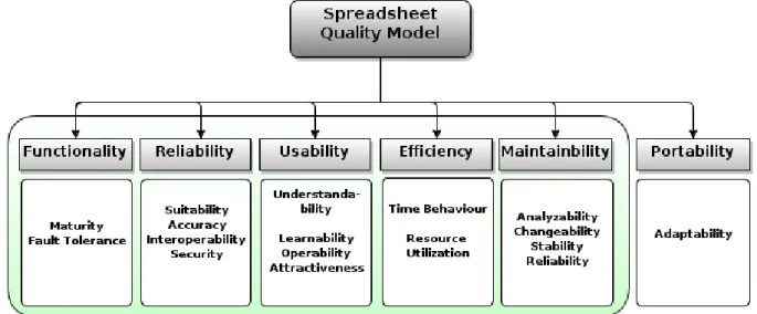
Due the current high complexity of spreadsheets and their frequent use [29], [16], they must be looked at like any other computer program from another programing language. This means that the use of metrics to measure and quantify entities in spreadsheets can be made like in other programing language. In fact, we can easily map the structure of a spreadsheet to an object oriented programing language: we just have to look at spread-sheets as a source code file, spread-sheets as classes, cells as methods and functions as statements. Knowing this Peixoto [25], created a quality model that we will be using to classify some spreadsheet metrics according five characteristics .

Figure 3.2:The Software Quality Model ISO/IEC 9126.

In the Figure. 3.2 we can see the software quality model created by Peixoto.

3.2.1 Functionality

This characteristic measures the ability of software to satisfy the user needs. This depends in four sub-characteristics:

• Suitability: measures if the spreadsheet has the right properties for the purpose it is meant. It is measured with metricsNumber of incongruencesandNumber of refer-ences to Blank Cells in Formulas;

(32)

14 CHAPTER 3. SOFTWARE QUALITY ASSESSMENT BASED ON METRICS measured using metrics asNumber of Output Cells with Errors/Bad Content,Number of incongruencesandNumber of Blank Cells referenced in Formulas;

• Interoperability: is the ability of two or more Sheets or components to exchange information and to use the information that has been exchanged. This uses metrics asData been exchanged between Sheets,Quantity of rightful formulas,Total of Cells with referencesandTotal of references;

• Security: verifies the existence of protected cells, sheets or even the entire workbook. This uses metrics as Protected Formulas, Protected Cell for Data only for reading

andUse Password to lock Workbook/Worksheets.

3.2.2 Reliability

This is the is capacity from a software to maintain its quality after a period of time and under specific conditions, it depends in three sub-characteristics;

• Maturity: evaluates if the spreadsheet is fully developed, for this metrics like: Num-ber of Labeled Rows/Columns that are empties,Number of Blank Cells in a matrix,

Number of Blank CellsandDifference between the Sheets that the Spreadsheet have, and the ones been used, are used.

• Fault Tolerance: is the property to continue operating properly in the event of one or more faults within some of its components, for this we use metrics likeNumber of Cells been referenced (Directly or indirectly) by many other CellsandNumber of Complex Formulas.

• Recoverability: is the capacity to restore a previous state, this characteristic does not apply because a spreadsheet can not restore itself.

3.2.3 Usability

Usability is the capability of a software being understood to the users, this characteristic depends in four sub-characteristics;

• Understandability: is the capacity of a spreadsheet being understood, for this we measure Different colors for different types of Data, Separate Input, Computation and OutputandNumber of Cells.

(33)

3.2. SPREADSHEET METRICS 15 • Learnability: evaluates the easiness for the user to use the spreadsheet, for this we use metrics Number of Cells, Different colors for different types of Data, Separate Input, Computation and Output, Number of Complex FormulasandAmount of Data being exchanged between Sheets.

• Operability: evaluates the capacity of work with the spreadsheet, for this we measure if it has Data Validation Drop Down Listsand Separated Inputs, Computation and Outputs.

• Attractiveness: measures how attractive is to the user, for this we measure the use of colors, the existence of Data Validation Drop Down Lists andSeparated Inputs, Computation and Outputs.

3.2.4 E

ffi

ciency

Efficiency is the ratio resources/performance of a software, this characteristic depends in two sub-characteristics.

• Time Behavior: estimates the computing time. For this we use the Number of V-Lookup’sand other search formulas, andNumber of Complex Formulas.

• Resources Utilization: estimates the resources needed. For this we use the Number of V-Lookup’s, theAmount of Blank-CellsandNumber of Complex Formulas.

3.2.5 Maintainability

Maintainability is the ease which a software can be modified/updated. This characteristic depends in four sub-characteristics.

• Analyzability: measure the capacity to analyze a spreadsheet, in order to conclude the effort needed for diagnosis deficiencies. In this we measure theNumber of Cells, if the data is or not well organized, the Number of References and the Number of Formulas.

• Changeability: evaluates the ease of change of a spreadsheet and concludes the effort needed for that modifications. In this characteristic we have to measureHow Well is the Data Organized, theNumber of Referenced Cellsand theNumber of Cells.

(34)

16 CHAPTER 3. SOFTWARE QUALITY ASSESSMENT BASED ON METRICS • Stability: evaluates how stable is a spreadsheet. For this we use the Number of Complex Formulasand the Number of Cells Referenced by Other Cells (directly or indirectly).

• Testability: evaluates how well can we test a spreadsheet. For this we only use the

Number of Formulas.

In Peixoto’s dissertation he also discusses portability, but we will not use it in the classifi-cation.

These classifications were also done in three levels, cell, sheet and spreadsheet.

From many of the metrics shown in Table A.1, Table A.2, Table A.3(Appendix A) we can infer new ones. For instance to measure the data density from one sheet we can somehow use the "#Cells" and the "#Blank Cells" to obtain a valid measure.

Cell Level:At the cell level Table A.1 we only have a few metrics, some of the metrics identified were the Fan-in, Fan-out, that together represent all the references from a cell, we also have references to empty cells and constants in formulas.

Sheet Level: At the sheet level we have a bigger set than on the cell because it uses all the results from the cell. Besides the metrics from the cell level we also have those in Table A.2.

Spreadsheet Level: At the spreadsheet level the set grows because, like at the sheet level, it inherit metrics from cell level, on spreadsheet happens the same but from the sheet level.

(35)

Chapter 4 Bad Smells

Summary:

In this chapter we first introduce the notion of smell in software presenting a taxonomy that uses a catalog of smells previously created by Fowler. We then discuss spreadsheet smells and present in detail our catalog of smells, the ones that we will use in the “SmellSheet Detective”. In this catalog we have statistical smells, type smells, input smells, functional dependencies smells and the ochiai smell.

“Code Smell: A code smell is a surface indication that usually corresponds to a deeper problem in the system.” Martin Fowler Website

The notion of "bad smell" was introduced to the computer science by Fowler in [11], and it emerged in his book because he felt the need to define when and where to apply internal structure improvements to a software. Since that was a complicated task he used "bad smells" as a flag to do it. A "bad smell" is an indicator of some possible bigger problem, like usually we say, something that smells.

This "new" notion is just an helpful tool and still depends on some previous criteria definition to be used. For instance the notion of what is a too big method can depend on the product, who analyzes it and the purpose of the analysis. Like the author says “no set of metrics rivals informed human intuition” [11].

In spite of the fact that this concept was thought to object oriented programing language, I think we can say that it fits in spreadsheets like a glove because in spreadsheets we almost

(36)

18 CHAPTER 4. BAD SMELLS never can tell if something is an error. Most of the times we point to something that does not feel right or something that could be done in a better way.

In the first part of this chapter we will see a list of smells that was introduced by Fowler in [11] but organized by Mantyla et al.[21] taxonomy. Then we will talk about smells in spreadsheets, were we will introduce the list of smells that we created and explain in detail how each one of them works.

4.1 Software Smells

Martin introduced the list of software smells in 2000. In 2003 Mantyla created a taxonomy to group them so it would be easier to understand them. This taxonomy is a posterior improvement of the taxonomy made to his thesis1_.

Group Smells

Long Methods Large Classes

The bloaters Long Parameter List

Long Methods Primitive Obsession Switch Statements The Object-Orientation Abusers Temporary Field

Refused Bequest

Alternative Classes with Different Interfaces Divergent Change

The Change Preventers Shotgun Surgery

Parallel Inheritance Hierarchies Lazy Class

Data Class

The Dispensables Duplicate Code

Dead Code

Speculative Generality Feature Envy

The Couplers Inappropriate Intimacy

Message Chains Middle Man

Table 4.1: Mantyla Taxonomy 1_http:_//_{www.soberit.hut.fi}_/_mmantyla_/_{badcodesmellstaxonomy.htm}

(37)

4.2. SPREADSHEET SMELLS 19

4.2 Spreadsheet Smells

The smells mentioned by Fowler are in single flat list, but Mantyla has created a taxonomy for all these smells. Similarly to what Mantyla has done we also grouped our smells by categories, five to be more specific: Statistical Smells, Type Smells,Content Smells, Func-tional Dependencies Based Smell,Ochiai Semlls. We will see how are they used by in our application.

Figure 4.1:Motivation example for smells

In the Figure 4.1 we present a spreadsheet, slightly adapted from one in the EUSES repository, where all kind of smells can be observed. All those smells will be automatically detected and flagged out by our tool “SmellSheet Detective”(Section 5.3).

4.2.1 Statistical Smells

This groups smells that are calculated through some kind of statistical analysis. In this category we only have theStandard Deviationsmell. The standard deviation smell detects cells that are outside the normal distribution.

(38)

20 CHAPTER 4. BAD SMELLS Detection

Most of the times when we fill a spreadsheet with numeric values we organize them either by row or column, and many times we introduce wrong values without noticing. So, the Standard Deviationsmell is detected by analyzing the spreadsheets row (column) by row (column) and flagging the values outside the normal distribution of 95,4% (two Standard deviations). In the detection of this smell neither formulas nor labels are taken into account.

Example

If we look to the Figure 4.1 we can see, for instance, that in the column B the standard deviation is of 2.369E8. Then the normal distribution values acceptable should be within [5.868E8, 1.534E9] and so in the cell B4 we detect a smell because it contains the value 123 that is outside that interval.

4.2.2 Type Smells

In this group of smells we have Empty Cell and Pattern Finder. They are both in this category because in both of them is made an analyze to the type of cell: Label, Number, Formula or Empty Cells.

• Empty Cell

Many times we forgot to fill some cells in spreadsheets that should be filled. In order to detect some of these cells we created theEmpty Cellsmell. TheEmpty Celllocates all the empty cells in the middle of others non empty cells, this means that if we have an empty line we will not find that line, or if we just have one label in the line we will see it just as a label.

Detection

In the detection of theEmpty Cellwhat we do is select all the possible windows of cells from each row (column) and verify if in that window there is an empty cell. In the Figure 4.2 we can see in green the cases where the smell is detected. For this smell we used a window of five cells because after looking to many spreadsheets we

(39)

Figure 4.2: Window of search in Empty Cell Smells

thought that was an acceptable size, but in order to guarantee that is the best size more tests should be made.

Example 4.2.1

Taking the example spreadsheet from Figure 4.1 we can see that the cells D2 and C6 have empty cells, and they are in the middle of cells with labels fulfilling what we said above, to have at least four cells surrounding it. Still from the same Figure we can see that more white cells exist, for instance in column I there are plenty, but these cells do not fulfill the condition. The analysis for this example is by column, if we look by row all the empty cells from the column I would be detected.

• Pattern Finder

The need of this smell came from the fact that many times we introduce values (nu-meric or labels) in the middle of formulas to simplify in the moment and then when reusing the spreadsheet we may forget to correct that "problem". In order to detect those cells we created the Pattern Finder, but not only for formulas. The Pattern Finder finds patterns in the sheet and if in some row we have only Numbers and in the middle of those numbers we find a Label/Empty Cell/Formula we point that cell as a smell.

(40)

The detection of thePattern Finder are quite similar to the one for theEmpty Cell. In fact they almost overlap each other because in this we also detect empty cells. The major differences between them is that in this smell we detect not only empty cells but also every other kind of cells, and, in this smell we use a smaller window, just four cells. We chose to use a smaller window because the occurrence of patterns without empty cells is quite smaller.

Once again more tests should be done in order to guarantee that this is a good size for the window.

Figure 4.3:Window of search in Pattern Finder Smells

In the Figure 4.3 we can see in detail how this detection is made.

Example 4.2.2

Taking the example spreadsheet from Figure 4.1 we can see that the cell G3 contains the value "o" so is from the type Label, and this cell is surrounded by Numbers creating a window of four cells like the one shown in Figure 4.3. This means that G3 is a smell, maybe that "o" is a typo and it should be a "0" (zero).

4.2.3 Content Smell

In this category we will have the smells found through the analysis of the content of the cell. We have putted in this category the String Distance smell and Reference to Blank Cellssmell.

(41)

4.2. SPREADSHEET SMELLS 23 • String Distance

When writing in a computer many times we make typo errors, so, to detect those we create theString Distance smell. In the String Distance smell we compare two strings and find if the minimum number of edits needed to transform one string into the other one.

Detection

The detection of this smell is made by using the algorithm created by Vladimir Lev-enshtein [20] in 1966,Levenshtein Distance.

The Levenshtein Distancecompares two strings and finds the minimum number of edits needed to transform one string into the other. So in order to do it we have to apply theLevenshtein Distance each string from a row (column) to all the others in the same row (column) and verify if the result is 1.

At first no verification to the strings was being done, and this was a problem be-cause, for instance if we had a spreadsheet with a row with alphabet all cells would be pointed out. So, we limited the comparison only to strings longer than three char-acters. The election of this value was made by looking into some spreadsheets and selecting the string length producing best results.

Example 4.3.1

ForString Distance, in the Figure 4.1 we can see a example of this smell. In the row C, the word in the cell C8 "SUNLIGHT DISH LIQUIDS" is the plural of the word in the cells C9 to C11 pointing to some probable typing error.

• Reference to Blank Cells

When we have a big spreadsheet with many formulas sometimes having a formula using an empty cell in the calculation may lead to problems in the output, so in order to detect those cells we created theReference to Blank Cells.

In theReference to Blank Cellssmell we identify if there is any formula with refer-ences to empty cells.

(42)

The detection of the Reference to Blank Cellssmell is made by walking all the for-mulas from the spreadsheet gathering all their references. Then, we just verify if each of the gathered reference is a reference to an empty cell flagging those that are.

Example 4.3.2

ForReference to Blank Cells, no example is presented in Figure 4.1 because it dis-plays the values and not the formulas used to compute each values. Thus, let us introduce a new example to illustrate this smell.

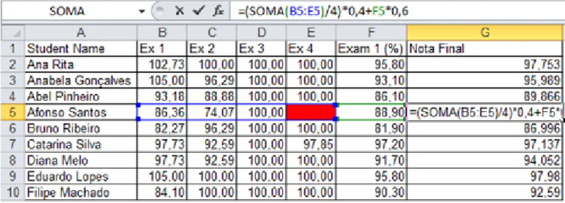
Figure 4.4:Reference to Blank Cells Example

So if we look to the Figure 4.4 we can see that it is in column G where the final grade of the students is calculated, the formula used to calculate the final grade is the one presented in G5 (=(SOMA(B:E)/4)*0,4+F*0,6) and in E5 we have an empty cell. Our “SmellSheet Detective”tool automatically detects this smell.

4.2.4 Functional Dependencies Based Smells

Similarly to what happens in databases, the existence of poor data, can be very costly for the companies who use them. Regarding that and because the problem as already been approached in the data mining field, we tried to adapt techniques used to identify dirty values in databases to spreadsheets.

In [4] it is described a technique to identify dirty values using Conditional Functional Dependencies (CFD), and this is one of the techniques that we will be using. Before we

(43)

4.2. SPREADSHEET SMELLS 25 start analyzing the algorithm let us introduce the concept of Functional Dependency (FD).

“Functional Dependency:are fundamental constraints that define the relation between attributes.”[19]

This means that one attribute A in the relation R only points to another attribute B, A→B. In other words this means that B is functionally dependent upon A, and every time that we have the attribute A it will imply the attribute B.

A CFD is the same as a FD but instead of use all the data, it only uses part of the data. Birth Country Nationality

China Chinese Spain Spanish Portugal Portuguese Portugal Portuguese Portugal Portuguese Portugal Portuguese

Table 4.2: Functional Dependency Example 1.

Birth Country Nationality

China Chinese Spain Spanish Portugal Portuguese Portugal Greek Portugal Portuguese Portugal Portuguese

Table 4.3: Functional Dependency Example 2.

In the Table 4.2 we can see that we have a relation between the Country of birth and the Nationality, more specifically we can see that when we have a citizen born in "Portugal" it is called as "Portuguese", so we can say that we have the FDBirthCountry →Nationality, so we have Portugal → Portuguese,China → ChineseandSpain→ Spanishas CFD’s. In the Table 4.3 we have Portugal→ Portuguese,Portugal →Greek,China→ Chinese

andSpain→Spanishas CFD’s.

Next we will see how to apply this in spreadsheets. Detection

In order to detect this smell some steps have to be taken:

1st Step - "Data collection"The first step towards the detection of this smell is the collec-tion of all the data from the spreadsheet. In this step we gather all the informacollec-tion contained in the all the cells from the spreadsheet. During this step we have to do an extra handling when dealing with formulas cells.

Because formulas are always different from cell to cell, even if they perform the same calculations we have to transform these "absolute" formulas into relative formulas. This

(44)

26 CHAPTER 4. BAD SMELLS means that, for instance, if we had the cell A11 with the absolute formula SUM(A1:A10) the correspondent relative formula would be SUM(R[-10]C:R[-1]C). With this all the for-mulas that perform the same operations and with the same range but in different cells they will have the same relative formula (same value for calculations).

2nd Step - "Matching Data" After the data collection we do an attribute lattice match, meaning that we match every column (row) with each other until we have a maximum of four matched columns (rows), depending on how we read the data from the spreadsheet.

Figure 4.5:Attribute match lattice.

To better understand how this match is done we should look tho the Figure 4.5 where each letter represents the name of one column. For instance the data from column A, matched with the data from the column B creates the new group of data AB that contains a subset where the data from both are the same. For instance, if we have A={{1,2,3},{4,5,6}and B={{1,2},{3},{4,5,6}then AB={{1,2},{3},{4,5,6}.

3o _{Step - "Identify Dirty Values"} _{After matching all the data we find all possible rules}

of the form [A,B] → C. In this step we have to make some manual configurations to adjust the quality of the dirty values returned. We have to define the support (θ), that is the minimum number of times that a FD must occur in order to be considered, and the maximum error frequency (α), that unlike the support, is the maximum number of times that a FD can occur in order to be considered a possible problem. These two variables are

(45)

4.2. SPREADSHEET SMELLS 27 going to be used as follow: first we walk all the xi⊂X and for each one we get the mapped

yi0_s ⊂ Y that we will use to verify if |ymax|

N ≥ θ and

|ys|

N ≤ α. In here the X and Y are the

partitions, for instance for the example in the Figure 4.6 if we have the candidate (X,Y)

= ((A,B,C,D),(A,B,C,D,E)), X would be the partition from (A,B,C,D) that in this case is {1,2,3,4,5,6,7,8,9,10,11,12} and Y would be the partition of (A,B,C,D,E) that in this case is {{1,2}{3,4,5,6,7,8,9,10,11,12}}. To better understand this you should read the paper [4]. In our tests we always usedθ=0.2 andα=0.1.

4o Step - "Ranking" In the previous step we obtain a list with many dirty values some of them can point to the same cells but using different CFDs, so in this step we sum the number of occurrences for each cell and rate them by frequency. This step is made to help us prioritizing the results.

Example 4.4

Figure 4.6:Conditional Functional Dependency Example

For instance if we take a look to the example in Figure 4.6 we can see that the data from the columns A,B,C andDis all the same. But in the column E we have two different values, "102" and "103". So, for the pink area we have the rule [A,B,C,D] → E103. This is the ymax and happens ten times, so we can calculate the support,θ = 10₁₂ = 0.8. For the

light blue area we have the rule [A,B,C,D] → E102, this happens two times and with this we can calculate the frequency, α= ₁₂2 = 0.16(6). After these calculations we just have to validate if they are according our reference values, the ones that we present in step three and we found as a smell the cells E1 and E2.

(46)

28 CHAPTER 4. BAD SMELLS

4.2.5 Ochiai Smells

The Ochiai smell is the application of the ochiai algorithm developed by Abreu et al.[1]. This algorithm is based in the ochiai similarity coefficient known from the biology domain and was introduced by Abreuet al.[1] in the context of fault localization, and previously adapted to spreadsheets by Riboira in the research for the SSaaPP project2_.

Detection

The algorithm adapted by Riboira receives as arguments a list of the cells detected by our smells and the spreadsheet being analyzed and with those it will calculate the probability of error from each cell and its dependents. By dependents we mean the references to other cells. For instance if we have a cell detected that is a formula that uses other cells the calculations of this smell will give ratings to all the cells implied.

Example 4.5

Figure 4.7:Ochiai Example

In the Figure 4.7 is presented an example where a pattern smell occurs: in cell C6 the pattern of constant values is broken by a formula (Section 4.2.2). So, applying the ochiai to that cell we have the output presented in the Figure 4.8

For this example where we only give the cell C6 to the ochiai as a smell, the output tell us that the cells A4, A5 and A6 have an 71% rate of being the source of the problem, and the cell C6 and B6 have 100%. This means that the cells in column A are used by the others to compute their values.

(47)

celulas ochiai: Sheet1!C6 [...\TESTE REF NULLS.xls]

NEW 'Sheet1'!A4 (71%) <<< WARNING! NEW 'Sheet1'!A5 (71%) <<< WARNING! NEW 'Sheet1'!A6 (71%) <<< WARNING! NEW 'Sheet1'!B6 (100%) <<< WARNING!

'Sheet1'!C6 (100%) <<< WARNING!

(48)

(49)

Chapter 5 Evaluation

Summary:

In this chapter we start by presenting the sample of spreadsheets that we will use in the study and we explain from where and how we select them. Then, we explain the classification model that will be used to classify the smells found. After we present the tool “SmellSheet Detective”and explain how it works, we explain its architecture and how it was built.

In the end we show and explain the results: these results start from the gen-eral to the particular, meaning that we show the global results and then we walk each category from the sample used and present results for each se-lected spreadsheet. In this process we analyze six spreadsheet categories, namely: database, financial, grades, homework, inventory and modeling.

“True genius resides in the capacity for evaluation of uncertain, hazardous, and conflicting information.” Winston Churchill

A successful evaluation of the results is always dependent on the data used on it: if we have poor data or an insufficient sample the results and conclusions taken may not be the more accurate. Knowing this, we searched for a big and representative set of spreadsheets to use in our analysis, the EUSES Corpus [17]. This set has already been used by others to perform analysis in spreadsheets [7].

(50)

32 CHAPTER 5. EVALUATION

5.1 EUSES Corpus

The EUSES Corpus is a repository built through a Google search by the name of the six ma-jor categories (Database, Financial, Grades, Homework, Inventory and Modeling ), leaving an initial sample of≈5600 spreadsheets that after some cleaning process made by the au-thors (for example, by removing the unusable and the duplicated ones) narrow the sample to≈4500 spreadsheets. From these 4500 we randomly selected 180 where categories and properties are presented in Table 5.1.

Category Vertically Horizontally Poor Data Total

Database 42 6 10 60 Financial 20 22 18 60 Grades 13 2 1 15 Homework 15 0 1 16 Inventory 9 1 4 14 Modeling 12 1 2 15

Table 5.1: Data orientation in spreadsheets.

More than half of the sample are spreadsheets from financial and database because these two categories were the ones we found more important and with the best data.

5.2 Classification Model

After the selection of the sample to be analyzed we had to define how the results would be measured and classified. For this we inspired ourselves in the technique used by the Software Improvement Group [15] and classified the smells in four levels:

• Level 1: In this level fit the cells that are week smells, things that may be a smell; • Level 2: In this level fit all the cells that we are almost certain that are smells but due

to the lack of understanding of the sheet we cannot guarantee it as a smell. • Level 3: In this level goes all the cells that we are sure that are smells.

• Not Smell: In this category goes all the wrong detections, because the tool did not work properly, or because the detection seem to be on purpose.

(51)

5.3. SMELLSHEET DETECTIVE - THE TOOL 33 The creation of this standard, made possible an uniform classification of the spreadsheets.

5.3 SmellSheet Detective - The Tool

In the analysis of the selected spreadsheet sample we used the tool “SmellSheet Detec-tive”which implements the smells introduced in the Chapter 4. This implementation was made in Java using the Google web toolkit [12] (GWT), the Apache POI [28] library and the Google libraries to work with spreadsheets from the Google Docs.

The use of Google in the application is because the technologies are evolving in the direction of the browser-based approach, and thus we had to keep up and do something according to it. Thus we built this tool that can work directly with a Google docs account [13].

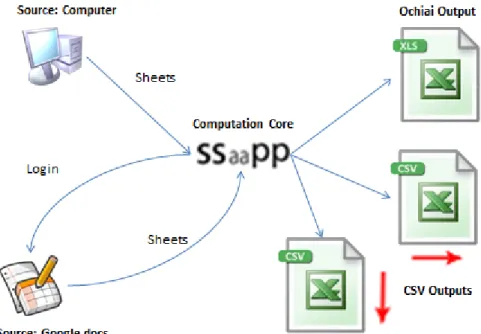
Figure 5.1:“SmellSheet Detective”Architecture.

Only having the Google docs as source of spreadsheets give rise to a security issue, because many of the spreadsheets may be confidential and thus we don’t want to share them with Google. For instance if one owns a company and wants to analyze the spreadsheets used by it one may feel that is giving secrets away. In order to surpass this problem we also have the possibility to directly analyze spreadsheets by uploading them to the tool

(52)

34 CHAPTER 5. EVALUATION instead of login in Google account. This functionality is just a few steps away of being full integrated.

With this we can describe the tool architecture as we see in Figure 5.1, where we have three major nodes: Spreadsheet source, Computation Core and CSV outputs.

In the Spreadsheet source, as we mentioned before we have the Google docs or direct upload. These two are the source from where the spreadsheets will be analyzed. If we use the Google docs source, we have to login in with our Google account credentials and select which spreadsheet to analyze. If we use the direct upload source, we just have to browse the spreadsheet in our computer and select it.

In the Computation Core is where all the smells defined will be applied to the selected spreadsheet(s).

Finally in the CSV outputs is were the outputs are created. Here we have three outputs, two csv files and one xls file. In the csvs we have the results for each smell by analyzing the data in two different ways, vertically and horizontally. In the xls file is where it will be presented the results of the ochiai analysis mentioned in Chapter 4.

5.4 Results

In the representation of the results instead of full spreadsheets, we selected ten sheets per category. This selection was made randomly. In some cases and since we were choosing the sheets randomly, we got empty sheets. In these cases we choosed another sheet to replace it. This happened just a few times because most of the spreadsheets have data; even if in some of them there was few data in the sheets or if they looked like a word document they had something to analyze. During the analysis of spreadsheets we realize that the organization of the data could be done in two ways: either we can put the data organized horizontally or vertically. This means that if the data was organized horizontally the values would be co-related column by column. If we look to the Figure 5.2 we see a financial spreadsheet where the expenses are presented for many years, putting these years side by side. So the relation that makes sense to evaluate is between those values side by side.

In the Figure 5.3 we see a grade spreadsheet that unlike what happens to the Figure 5.2 the values that make sense to relate are the grades for each problem. So in this case we have a vertical organization.

(53)

5.4. RESULTS 35

Figure 5.2: Horizontal Organization Data Example. (Adapted from FIN_hospitaldataset2002 spreadsheet).

Figure 5.3: Vertical Organization Data Example. (Adapted from GRD_483_grades_web spreadsheet).

Because of these two types of organization we decided to classify the sample used. To do so, we opened all the spreadsheets one by one and that make us realize that most of the spreadsheets had poor data in it: some were empty forms and others some sort of manuals or catalogs were the data was mostly labels, so, we decided to identify some of these but keeping a very permissive criteria because in spite we thought the data was poor, it was still possible to analyze them. This lead to the fact that many of the spreadsheets characterized as horizontal/vertical still hadn’t relevant data. The numbers of this classification can be seen in the Table 5.1.

Next we will see the results for each of the six categories from the EUSES corpus. During the presentation of the results first we will see the individual outputs for each sheet and highlight some of the more relevant results. In the presentation of the results we will hide the smells that had no cells flagged.

Then we will discuss the global results where we will group the results of all sheets and make a statistical analysis to them. This statistical analysis will be done by level, and smell and the values presented will always be an approximation because they will remain accurate enough and will simplify the reading.

(54)

36 CHAPTER 5. EVALUATION

5.4.1 Database Sheets

With 60 spreadsheets theDatabasecategory is one of the two biggest samples that we have used. Because this category mostly included spreadsheets similar to databases, most of the cells were numeric and label values. The caption of each table is the name of the sheet with the following format: DB_spreadsheet name sheet name. In the next sections the tables are named likewise, just changing the first letters to meet the corresponding category. Also, in the tables when the values occur followed by “matches” means that instead of number of cells are the number of combinations founded, this only happens in the string distance smell because the smell compares the cells two by two.

Results P P P P P P P P P P_P Smell Level

Level 1 Level 2 Level 3 Not Smell

Std. Dev. Cells 9 0 0 1

F.D. Cells 2 1 0 0

Table 5.2: DB_basicdata HAFO Permits.

P P P P P P P P P P_P Smell Level

Empty Cells 2 0 0 21

Patterns 2 0 0 38

Table 5.3: DB_cattrainchecklist Sheet1.

String Dist. 0 0 0 6 Matches

(55)

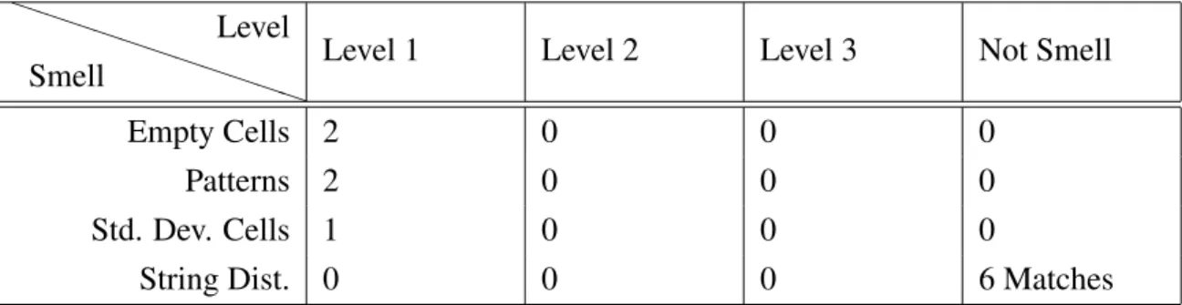
5.4. RESULTS 37 P P P P P P P P P P_P Smell Level

Empty Cells 2 0 0 0

Patterns 2 0 0 0

Table 5.5: DB_SteamTool 3. STEAM SYSTEM PROFILING.

Empty Cells 5 0 0 9

Patterns 5 0 0 9

F.D. Cells 2 4 1 0

Table 5.6: DB_NamingConventionDataS#A855B Summary.

Empty Cells 0 1 0 0

Patterns 0 1 0 0

Table 5.7: DB_rmomatrix MATRIX.

Empty Cells 0 0 0 15

Patterns 0 0 0 29

F.D. Cells 0 2 0 0

(56)

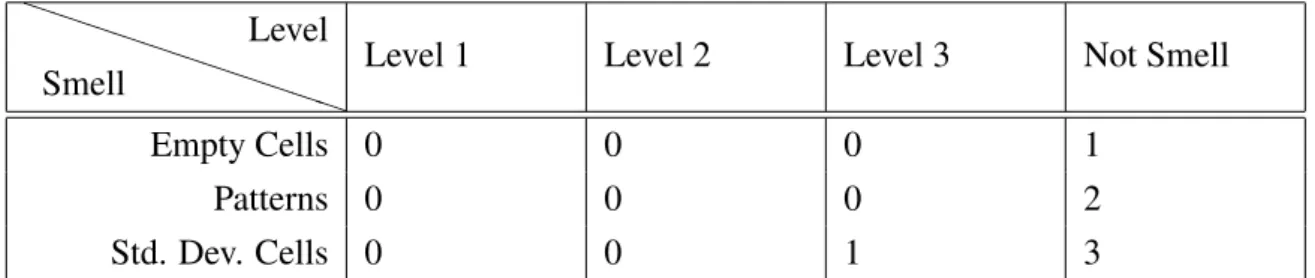
38 CHAPTER 5. EVALUATION P P P P P P P P P P_P Smell Level

Empty Cells 0 0 0 1

Patterns 0 0 0 2

Table 5.9: DB_Population Pop.l1.

Table 5.10: DB_dab1 Sheet3.

Besides the results showed above, we also analyzed the sheet“DB_2004_admin_plan Goal C”but because in this sheet all the results obtained were zero we did not create a table for it.

From the results above, some got our attention. For instance, in Table 5.4 and Table 5.10 none of the detected cells were considered smells, making these sheets the ones with worst percentage results in the category. On the other hand, Table 5.2 with ≈85% of the cells flagged level 1 and ≈8% as level 2 is where we find the best percentage results for the category.

Another thing we must notice is that in spite of for Table 5.4 the percentage results are the worst, the Table 5.3 and Table 5.8 the number of not smells is substantially higher.

Discussion

Now we will see the general results for the Database category and discuss some of the more relevant findings.

(57)

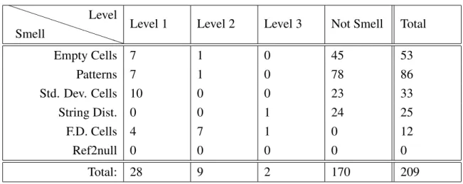
5.4. RESULTS 39 P P P P P P P P P P_P Smell Level

Level 1 Level 2 Level 3 Not Smell Total

Empty Cells 7 1 0 45 53 Patterns 7 1 0 78 86 Std. Dev. Cells 10 0 0 23 33 String Dist. 0 0 1 24 25 F.D. Cells 4 7 1 0 12 Ref2null 0 0 0 0 0 Total: 28 9 2 170 209

Table 5.11: Database Result Totals.

In the Table 5.11 is presented the total values for each smell and the total values by level from all the sheets seen previously.

Empty Cells 13% 2% 0% 85% Patterns 8% 1% 0% 91% Std. Dev. Cells 30% 0 % 0% 70% String Diff. 0% 0% 4% 96% F.D. Cells 33% 58% 8% 0% Ref2null 0% 0 % 0% 0% Total: 13% 4% 1% 81%

(58)

Empty Cells 25% 11% 0% 26% Patterns 25% 11% 0% 46% Std. Dev. Cells 36% 0 % 0% 14% String Diff. 0% 0% 50% 14% F.D. Cells 14% 78% 50% 0% Ref2null 0% 0 % 0% 0%

Table 5.13: Database Statistical Result by Level.

Observing the Tables 5.11, 5.12 and 5.13 the first thing that we notice is that no references to empty cells have been found. This happens because in this category, from the ten selected sheets, the data was mainly label and numeric values, not leaving room for this smell.

Another thing we can see in the tables is that the patterns and the empty cells are the smells that happen more often and they have some overlap results. This happens because these two smells have much in common. In fact the patterns will found almost all the results that the empty cells do, and some more.

Still from the tables we can see that for the functional dependencies smell none of the findings was considered not a smell. This is easy to understand why: like we have talked in Section 4.2.4 the algorithm used to detect these smells was adapted from the databases, and being this category the databases category was expected that the results were well behaved. Also if we look to Table 5.12 we can see that most of the detected cells (≈81%) were not considerate as smells, but we must consider that from these≈81% of cells≈72% were either empty cells or patterns that were almost overlapped smells. This happens so much because in this category many sheets were really like databases where null values are al-lowed and in the spreadsheets were represented by empty cells. Still from these≈81% cells ≈14% where string differences where the difference was in a numeric value.

5.4.2 Financial Sheets

Like theDatabasecategory theFinancialis the other big sample with a total of 60 spread-sheets. But unlike theDatabase this category is more complex in terms of types of data having a little bit of all cell types (Formulas, Constants and Labels).

(59)

5.4. RESULTS 41 Results P P P P P P P P P P_P Smell Level

Empty Cells 0 0 0 4

Patterns 2 0 0 0

String Diff. 0 0 0 7 Matches

Ref2null 6 0 0 0

Table 5.14: FIN_CMSAauditreport2002_2003 Sheet1.

P P P P P P P P_P P_P Smell Level

Empty Cells 0 2 0 0 Patterns 0 2 0 0 Std. Dev. Cells 0 0 0 18 String Diff. 0 0 0 3 Matches F.D. Cells 0 0 3 0 Ref2null 0 0 4 0

Table 5.15: FIN_FinalAnnexFSSN06001 Annex3.

Empty Cells 0 0 0 2

Patterns 0 0 0 2

Ref2null 8 0 0 0

(60)

Empty Cells 3 0 0 6

Patterns 4 0 0 30

String Diff. 0 0 0 3 Matches

Table 5.17: FIN_Financial%20Compariso#A7ED8 Financial Comparison Analysis.

P P P_P P P P P P P_P Smell Level

Ref2null 0 0 1 6

Table 5.18: FIN_finrpt00 Five Year Review.

Empty Cells 0 0 0 6

Patterns 0 0 0 6

Table 5.19: FIN_income-statement Income Statement.

P P P P P P P P P_P P Smell Level

Ref2null 1 1 0 0

Table 5.20: FIN_MATHCOUNTS%20Financial Sheet1.

Empty Cells 0 0 0 4

(61)

5.4. RESULTS 43 Table 5.21: FIN_hospitaldataset2002 MEMORIAL.

Beside the sheets presented above we also analyzed the sheets“FIN_clienttemplate Finan-cial Diagnostics” and“FIN_financial-greece_el GR”, but since the results obtained were all zero no tables were created.

From the result tables presented we can notice that, for instance, for Table 5.19 and Table 5.21 all the flagged cells were considered not smells making them the sheets with the worst results from the sample. On the other hand Table 5.20 all the cells were correctly flagged and therefore this is the sheet with the best results.

Other result that we must highlight is the pattern smell in Table 5.17 where 30 cells were categorized as not smell. This value is quite high specially if we compare it to the rest of the values.

We also must underline the standard deviation smell in Table 5.15 where we also ob-tained a quite high value again, specially if compared to the other values.

Discussion

Now we will see the general results obtained in the Financial category and point some interesting facts that can be extracted from them.

Level 1 Level 2 Level 3 Not Smell Total

Empty Cells 3 2 0 22 27 Patterns 6 2 0 54 62 Std. Dev. Cells 2 0 0 33 35 String Diff. 0 0 0 13 13 F.D. Cells 0 0 3 0 3 Ref2null 9 1 7 6 23 Total: 20 5 10 128 163

(62)

Empty Cells 11% 7% 0% 81% Patterns 10% 3% 0% 87% Std. Dev. Cells 6% 0 % 0% 94% String Diff. 0% 0% 0% 100% F.D. Cells 0% 0% 100% 0% Ref2null 39% 4 % 30% 26% Total: 12% 3% 6% 79%

Table 5.23: Financial Statistical Result by Smell.

Empty Cells 15% 40% 0% 17% Patterns 30% 40% 0% 42% Std. Dev. Cells 10% 0 % 0% 26% String Diff. 0% 0% 0% 10% F.D. Cells 0% 0% 30% 0% Ref2null 45% 20 % 70% 5%

Table 5.24: Financial Statistical Result by Level.

Unlike what happens in the previous category in which we did not find one type of smells, in the Financialcategory we have results for every type of smell. Still, by observing Ta-ble 5.22, TaTa-ble 5.23 and TaTa-ble 5.24 there are some facts that can be observed. One thing that can be easily observed from the tables is that in the string distance smell all the flagged matches were considered not smells. In spite of the detected smells were all wrong, they can be easily corrected because all of them were either numeric values with a dollar mark associated or index labels where the difference was in the number of the index.

Another thing that we can see is that unlike the string distance smell, in the functional dependencies smell all the flagged cells are level 3. This may lead to conclude that this smell works very well for this category but because all the cells came from the same sheet (Table 5.15) we just can say that for that sheet this smell worked perfectly. In fact in this

Spreadsheet smells

acknowledgements

Resumo

Abstract

Contents

List of Figures

List of Tables

Chapter 1

Introduction

1.1

Structure of the dissertation

Chapter 2

State of the Art

Chapter 3

Software Quality Assessment Based on

Metrics

3.1

Program Metrics

3.1.1

Why measure things?

3.1.2

How to measure things?

3.1.3

Software Metrics

3.2

Spreadsheet Metrics

3.2.1

Functionality

3.2.2

Reliability

3.2.3

Usability

3.2.4

E

ffi

ciency

3.2.5

Maintainability

Chapter 4

Bad Smells

4.1

Software Smells

4.2

Spreadsheet Smells

4.2.1

Statistical Smells

4.2.2

Type Smells

4.2.3

Content Smell

4.2.4

Functional Dependencies Based Smells

4.2.5

Ochiai Smells

Chapter 5

Evaluation

5.1

EUSES Corpus

5.2

Classification Model

5.3

SmellSheet Detective - The Tool

5.4

Results

5.4.1

Database Sheets

5.4.2

Financial Sheets