Learning Effective Binary Representation with
Deep Hashing Technique for Large-Scale
Multimedia Similarity Search
Gengshen Wu
School of Computing and Communications
Lancaster University
A thesis submitted for the degree of
Doctor of Philosophy
Declaration
This thesis has not been submitted in support of an application for another degree at this or any other university. It is the result of my own work and includes nothing that is the outcome of work done in collaboration except where specifically indicated. Many of the ideas in this thesis were the product of discussion with my supervisor Dr. Jungong Han.
Parts of this thesis have been publised previously in the following publications: [Chapter 3]
G. Wu, Z. Lin, G. Ding, Q. Ni and J. Han. “On Aggregation of Unsupervised Deep Binary Descriptor with Weak Bits,” IEEE Transactions on Image Processing, 2020. (Accepted)
[Chapter 4]
G. Wu, L. Liu, Y. Guo, G. Ding, J. Han, J. Shen, and L. Shao. “Unsupervised deep video hashing with balanced rotation,” in International Joint Conference on Artificial Intelligence, 2017, pp. 3076-3082.
G. Wu, J. Han, Y. Guo, L. Liu, G. Ding, Q. Ni, and L. Shao. “Unsupervised Deep Video Hashing via Balanced Code for Large-Scale Video Retrieval,” IEEE Transac-tions on Image Processing, vol. 28, no. 4, pp. 1993-2007, April 2019.
[Chapter 5]
G. Wu, Z. Lin, J. Han, L. Liu, G. Ding, B. Zhang, and J. Shen. “Unsuper-vised Deep Hashing via Binary Latent Factor Models for Large-scale Cross-modal Retrieval,” in International Joint Conference on Artificial Intelligence, 2018, pp. 2854-2860.
G. Wu, J. Han, Z. Lin, G. Ding, B. Zhang and Q. Ni. “Joint Image-Text Hashing for Fast Large-Scale Cross-Media Retrieval Using Self-Supervised Deep Learning,” IEEE Transactions on Industrial Electronics, vol. 66, no. 12, pp. 9868-9877, Dec. 2019.
Gengshen Wu September, 2020
iii
Acknowledgements
First of all, I would like to thank my supervisor Dr. Jungong Han, who allowed me to complete my Ph.D. study at Lancaster University. Under his supervision, we enjoy unprecedented freedom of research in the aca-demic field. He has been providing me with continuous support, insightful guidance, inspiring ideas and shaping me to be a qualified researcher. I would like to extend the sincerest thanks to the following people, who have all helped in the completion of this thesis.
I would like to thank Prof. Qiang Ni, Dr. Matthew Broadbent, Dr. Zheng Wang and Dr. Hossein Rahmani in our school for their kind support and suggestions.
I would like to thank the previous and current visiting scholars in our lab, including Prof. Heng Liu, Prof. Hai Li, and Dr. Yi Liu, Dr. Yuanjun Huang and Dr. Shanfeng Wang for their helpful discussions and research ideas.
I would also like to thank my co-authors, Prof. Ling Shao, Prof. Guiguang Ding, Dr. Jialie Shen, Dr. Baochang Zhang, Dr. Yuchen Guo, Dr. Zijia Lin and Dr. Li Liu, who have improved my research outcomes from many aspects.
I would like to thank Dr. Yi Zhou, who introduced me to Dr. Jungong Han as a Ph.D. candidate and let the story began.
I would also like to thank all previous members from Northumbria sity, Lancaster University, Warwick University, and East Anglia Univer-sity, including Dr. Yuming Shen, Dr. Bingzhang Hu, Dr. Yijun Shen, Dr. Jingtian Zhang, Dr. Shanfeng Hu, Dr. Tianhao Guo, Dr. Zheming Zuo, Dr. Xiaowei Gu, Dr. Zhaoxu Yang, Dr. Haiyang Liu, Dr. Bintao He, Dr. Ning Gao, Dr. Wenda Tang, Shoujiang Xu, Jiaojiao Zhao, Shuo Zhang, Yao Zhang, Matthew Gingfung Yeung, Binbin Su, Peng Cheng, Yunqi
iv
Miao, Mingqi Gao, and Zhuang Shao. Thank them for their friendly help during my Ph.D. study.
I would like to thank Northumbria University and Lancaster University, they provided the financial support for me to complete my Ph.D. research. Many thanks to my family for their unconditional support during my Ph.D. study.
Abstract
The explosive growth of multimedia data in modern times inspires the research of performing an efficient large-scale multimedia similarity search in the existing information retrieval systems. In the past decades, the hashing-based nearest neighbor search methods draw extensive attention in this research field. By representing the original data with compact hash code, it enables the efficient similarity retrieval by only conducting bitwise operation when computing the Hamming distance. Moreover, less memory space is required to process and store the massive amounts of features for the search engines owing to the nature of compact binary code. These advantages make hashing a competitive option in large-scale visual-related retrieval tasks. Motivated by the previous dedicated works, this thesis focuses on learning compact binary representation via hashing techniques for the large-scale multimedia similarity search tasks. Particularly, several novel frameworks are proposed for popular hashing-based applications like a local binary descriptor for patch-level matching (Chapter 3), video-to-video retrieval (Chapter 4) and cross-modality retrieval (Chapter 5). This thesis starts by addressing the problem of learning local binary de-scriptor for better patch/image matching performance. To this end, we propose a novel local descriptor termed Unsupervised Deep Binary De-scriptor (UDBD) for the patch-level matching tasks, which learns the transformation invariant binary descriptor via embedding the original vi-sual data and their transformed sets into a common Hamming space. By
imposing a `2,1-norm regularizer on the objective function, the learned
binary descriptor gains robustness against noises. Moreover, a weak bit scheme is applied to address the ambiguous matching in the local binary descriptor, where the best match is determined for each query by compar-ing a series of weak bits between the query instance and the candidates, thus improving the matching performance.
vi
Furthermore, Unsupervised Deep Video Hashing (UDVH) is proposed to facilitate large-scale video-to-video retrieval. To tackle the imbalanced distribution issue in the video feature, balanced rotation is developed to identify a proper projection matrix such that the information of each dimension can be balanced in the fixed-bit quantization, thus improv-ing the retrieval performance dramatically with better code quality. To provide comprehensive insights on the proposed rotation, two different video feature learning structures: stacked LSTM units (UDVH-LSTM) and Temporal Segment Network (UDVH-TSN) are presented in Chapter 4.
Lastly, we extend the research topic from single-modality to cross-modality retrieval, where Self-Supervised Deep Multimodal Hashing (SSDMH) based on matrix factorization is proposed to learn unified binary code for dif-ferent modalities directly without the need for relaxation. By minimiz-ing graph regularization loss, it is prone to produce discriminative hash code via preserving the original data structure. Moreover, Binary Gra-dient Descent (BGD) accelerates the discrete optimization against the bit-by-bit fashion. Besides, an unsupervised version termed Unsupervised Deep Cross-Modal Hashing (UDCMH) is proposed to tackle the large-scale cross-modality retrieval when prior knowledge is unavailable.
List of Publications
Conference Papers
1. G. Wu, L. Liu, Y. Guo, G. Ding, J. Han, J. Shen, and L. Shao. “Unsupervised deep video hashing with balanced rotation,” in Inter-national Joint Conference on Artificial Intelligence, 2017, pp. 3076-3082. (CORE A* conference)
2. G. Wu, Z. Lin, J. Han, L. Liu, G. Ding, B. Zhang, and J. Shen. “Unsupervised Deep Hashing via Binary Latent Factor Models for Large-scale Cross-modal Retrieval,” in International Joint
Confer-ence on Artificial IntelligConfer-ence, 2018, pp. 2854-2860. (CORE A*
conference)
Journal Papers
1. G. Wu, J. Han, Y. Guo, L. Liu, G. Ding, Q. Ni, and L. Shao. “Unsupervised Deep Video Hashing via Balanced Code for Large-Scale Video Retrieval,” IEEE Transactions on Image Processing, vol. 28, no. 4, pp. 1993-2007, April 2019. (IF: 6.79)
2. G. Wu, J. Han, Z. Lin, G. Ding, B. Zhang and Q. Ni. “Joint Image-Text Hashing for Fast Large-Scale Cross-Media Retrieval Us-ing Self-Supervised Deep LearnUs-ing,” IEEE Transactions on Industrial Electronics, vol. 66, no. 12, pp. 9868-9877, Dec. 2019. (IF: 7.503) 3. G. Wu, Z. Lin, G. Ding, Q. Ni and J. Han. “On Aggregation of
Un-supervised Deep Binary Descriptor with Weak Bits,” IEEE Transac-tions on Image Processing, 2020. (IF: 6.79; Accepted)
viii
Co-Authored Papers
1. Y. Qi, J. Gu, Y. Zhang, G. Wu, and F. Wang. “Supervised Deep
Semantics-Preserving Hashing for Real-Time Pulmonary Nodule Im-age Retrieval,” Journal of Real-Time ImIm-age Processing, 2020.
2. S. Zhang,G. Wu, and J. Han. “Pruning Filter with Attention
Mech-anism for Deep Networks Compression on Remote Sensing Image,” Remote Sensing, 2020.
Contents
Declaration ii
Acknowledgements iii
Abstract v
List of Publications vii
List of Tables xiv
List of Figures xvi
List of Acronyms xx
List of Algorithms xxv
1 Introduction and Background Theory 1
1.1 Research Background . . . 1
1.2 Fundamental Theory of Hashing Technique . . . 4
1.2.1 Hash Function . . . 4
1.2.2 Objective Function Construction . . . 6
1.2.3 Optimization Strategy . . . 7
1.2.3.1 Continuous Relaxation . . . 7
1.2.3.2 Alternative Optimization . . . 8
1.2.3.3 Coordinate Descent . . . 8
1.2.4 Fast Similarity Search with Hash Code . . . 9
1.2.4.1 Hash Code Ranking . . . 9
1.2.4.2 Hash Table Lookup . . . 10
1.2.5 Evaluation Metrics . . . 11
1.2.5.1 Precision@K . . . 11
CONTENTS x
1.2.5.2 Mean Average Precision . . . 11
1.2.5.3 Precision-Recall Curve . . . 12
1.2.5.4 Receiver Operating Characteristic Curve . . . 12
1.3 Research Problems and Challenges . . . 13
1.3.1 Local Binary Descriptor . . . 13
1.3.2 Video Hashing . . . 15
1.3.3 Cross-Modality Hashing . . . 16
1.4 Overview of Contributions . . . 19
1.5 Thesis Outline . . . 21
2 Literature Review on Hashing-Based Similarity Search 23 2.1 Single-Modality Similarity Search . . . 23
2.1.1 Image Hashing . . . 24
2.1.2 Local Feature Descriptor . . . 27
2.1.2.1 Handcrafted Feature Descriptors . . . 27
2.1.2.2 Learning-Based Feature Descriptors . . . 28
2.1.3 Video Hashing . . . 30
2.1.3.1 Early Video Hashing . . . 30
2.1.3.2 Deep Learning Based Video Hashing . . . 31
2.2 Cross-Modality Similarity Search . . . 33
2.2.1 Supervised Cross-Modal Hashing . . . 33
2.2.2 Unsupervised Cross-Modal Hashing . . . 36
2.3 Chapter Summary . . . 37
3 Unsupervised Deep Binary Descriptor 39 3.1 Introduction . . . 39
3.2 Methodology . . . 43
3.2.1 Framework Overview . . . 43
3.2.2 Learning Unified Binary Descriptor . . . 44
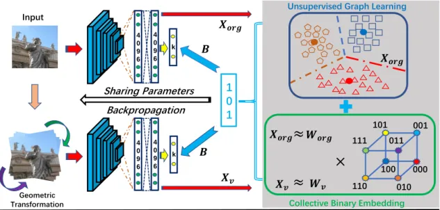
3.2.2.1 Collective Binary Embedding . . . 44
3.2.2.2 Unsupervised Graph Learning . . . 45
3.2.3 Optimization Algorithm . . . 46
3.2.3.1 Wv Step . . . 47
3.2.3.2 B Step . . . 47
3.2.3.3 αv Step . . . 48
3.2.4 Generating Out-of-Sample Binary Descriptor . . . 49
CONTENTS xi 3.3 Experiment . . . 51 3.3.1 Dataset Descriptions . . . 51 3.3.1.1 Brown . . . 51 3.3.1.2 Cifar-10 . . . 51 3.3.1.3 HPatches . . . 52 3.3.2 Implementation Details . . . 52
3.3.3 Comparisons with State-of-The-Arts . . . 52
3.3.3.1 Results on Brown Dataset . . . 52
3.3.3.2 Results on Cifar-10 Dataset . . . 55
3.3.3.3 Results on HPatches Dataset . . . 57
3.3.4 Further Analysis . . . 58
3.3.4.1 Ablation Study . . . 58
3.3.4.2 Transformation Invariance . . . 59
3.3.4.3 Weak Bit Study . . . 60
3.3.4.4 Loss Term . . . 60
3.3.4.5 Parameter Analysis . . . 61
3.4 Chapter Summary . . . 61
4 Unsupervised Deep Video Hashing 63 4.1 Introduction . . . 63
4.2 Proposed Unsupervised Deep Video Hashing . . . 66
4.2.1 Deep Video Feature Learning . . . 67
4.2.1.1 UDVH-LSTM . . . 67
4.2.1.2 UDVH-TSN . . . 69
4.2.2 Feature Embedding with Pseudo Labels . . . 70
4.2.3 Balanced Rotation . . . 71
4.2.4 Objective Function and Optimization . . . 73
4.2.4.1 RStep . . . 75 4.2.4.2 B Step . . . 76 4.2.4.3 Θ Step . . . 76 4.2.5 Complexity Analysis . . . 77 4.2.6 Discussion . . . 78 4.3 Experiments . . . 79
4.3.1 Datasets and Experimental Setting . . . 79
4.3.1.1 FCVID . . . 79
CONTENTS xii
4.3.1.3 ActivityNet . . . 80
4.3.2 Baselines . . . 80
4.3.3 Implementation Details . . . 80
4.3.4 Evaluation Metrics . . . 81
4.3.5 Comparison with State-of-The-Arts . . . 82
4.3.5.1 Results from UDVH-LSTM . . . 83
4.3.5.2 Results from UDVH-TSN . . . 84
4.3.5.3 Discussion . . . 88 4.3.6 Architecture Investigation . . . 89 4.3.6.1 Parameter Analysis . . . 89 4.3.6.2 Binarization Investigation . . . 90 4.3.6.3 Loss Function . . . 90 4.3.7 Feature Selection . . . 92 4.3.8 Efficiency Analysis . . . 93 4.4 Chapter Summary . . . 94
5 Deep Cross Modal Hashing 97 5.1 Introduction . . . 97
5.2 Proposed Method . . . 101
5.2.1 Problem Definition . . . 101
5.2.2 Deep Architecture . . . 102
5.2.3 Regularized Binary Latent Model . . . 103
5.2.3.1 Binary Reconstruction Loss . . . 103
5.2.3.2 Graph Regularization Loss . . . 104
5.2.4 Deep Hash Function Learning . . . 104
5.2.5 Objective Function and Optimization . . . 105
5.2.5.1 Ui Step . . . 105
5.2.5.2 B Step . . . 105
5.2.5.3 αi Step . . . 107
5.2.5.4 Θi Step . . . 107
5.2.6 Computational Complexity . . . 108
5.2.7 Extension to Unsupervised Cross-Modal Hashing . . . 108
5.3 Experiment . . . 109
5.3.1 Dataset Descriptions . . . 110
5.3.1.1 Wiki . . . 110
CONTENTS xiii
5.3.1.3 NUS-WIDE . . . 110
5.3.2 Experiment Settings . . . 110
5.3.3 Results and Analysis . . . 112
5.3.3.1 Architecture Investigation . . . 112
5.3.3.2 Overall Comparisons with Baselines . . . 112
5.3.3.3 Top-5 Retrieved Examples for SSDMH . . . 113
5.3.3.4 Effect of Training Data Size . . . 116
5.3.3.5 Parameter Sensitivity Analysis . . . 119
5.3.3.6 Convergence Study . . . 119
5.3.3.7 BGD versus One Entry . . . 119
5.3.3.8 Training Efficiency . . . 121
5.3.4 Quantitative Results for UDCMH . . . 122
5.3.4.1 Comparison With State-of-The-Arts . . . 122
5.3.4.2 Training Data Size . . . 125
5.4 Chapter Summary . . . 125
6 Conclusions and Future Work 126 6.1 Thesis Summary . . . 126
6.1.1 Unsupervised Deep Binary Descriptor . . . 126
6.1.2 Unsupervised Deep Video Hashing . . . 127
6.1.3 Deep Cross-Modal Hashing . . . 127
6.2 Future Research Topics . . . 128
6.2.1 Hashing for Deep Binary Neural Network . . . 128
6.2.2 Online Hashing . . . 128
6.2.3 Fine-Grained Retrieval with Weighted Hamming Distance . . 129
6.2.4 Fast Person Re-Identification . . . 130
List of Tables
3.1 Mathematical symbols and their short descriptions. . . 44
3.2 Comparison of the proposed UDBD to the state-of-the-art binary
de-scriptors in terms of FPR@95% on Brown dataset. Dim, SP and USP
denote dimension, supervised and unsupervised, respectively. † and ‡
indicate the train and testing subsets. The results from SIFT and su-pervised methods are provided as references. Bold values are the best
results in unsupervised binary descriptors. . . 53
3.3 mAP of Top 1,000 (%) returned images at different code length from
various unsupervised descriptors on Cifar-10 dataset. Bold values are
the best results. . . 56
3.4 Precision at Top 1 on Cifar-10 dataset when using DeepBit, BinGAN,
GraphBit and UDBD at different bit sizes. . . 56
3.5 Comparison of the proposed UDBD to the state-of-the-art descriptors
in terms of mAP (%) on HPatches dataset. Dim, SP and USP denote dimension, supervised and unsupervised, respectively. The real-valued descriptor (SIFT) and the supervised methods are provided as refer-ences. Bold values are the best results in unsupervised binary descriptors. 58
3.6 Ablation study on Brown (FPR@95%): Liberty→Notre Dame and
Yosemite→Liberty, HPatches: matching (mAP) and Cifar-10 at 64 bits
(mAP@1000) when γ = 0 (i.e., UDBDγ=0) and β = 0 (i.e., UDBDβ=0). 59
3.7 mAP variations on HPatches with/without using weak bit scheme
(UDBD‡/UDBD†). Bold values show the best results. . . 60
3.8 Performance variations on Brown (FPR@95%): Notre Dame→Liberty
and Liberty→Notre Dame, HPatches: matching (mAP) at 256 bits,
and Cifar-10 at 32 bits (mAP@1,000) when using `2,1-norm and `2,2
-norm loss terms. . . 61
4.1 Mathematical symbols and their short descriptions. . . 67
LIST OF TABLES xv
4.2 The network configurations UDVH-LSTM and UDVH-TSN. Other
lay-ers like pooling and activation are omitted for concise descriptions. . . 70
4.3 mAP@20 of different cluster numbers at 128 bits on three datasets
under UDVH-LSTM and UDVH-TSN. . . 89
4.4 mAP@K of 128 bits when using various banarization schemes
sepa-rately in the code learning of UDVH-LSTM and UDVH-TSN. . . 91
4.5 mAP@20 at 128 bits when applying various loss functions accordingly
during the hash function learning of UDVH-LSTM and UDVH-TSN. 92
4.6 The training time at various code lengths on FCVID when using SSTH,
UDVH-LSTM and UDVH-TSN. The time unit for network training is
hour (h) and the rest processes are reported in second (s). . . 94
5.1 The Network Configurations for Two Modalities. Other layers like
pooling and activation are omitted for concise descriptions. . . 101
5.2 Mathematical symbols and their short descriptions. . . 102
5.3 mAP results at the code length of 128 when involving various loss terms
deployed in the proposed method: SSDMHbrl and SSDMHbrl+grl. . . . 112
5.4 The variations on αi(i= 1,2) during the optimization iteration at 128
bits on three datasets. αi are initialized as 0.5. . . 113
5.5 mAP results for Image→Text and Text→Image tasks on three datasets
at various code lengths (bits) when using different methods. The best
performance is shown in boldface. . . 114
5.6 Effect of training data size on MIRFlickr and NUS-WIDE at the code
length of 64. . . 119
5.7 Time costs (in seconds) in the training processes of SSDMH on three
datasets at 128 bits for one loop (T). . . 121
5.8 mAP results for Image→Text and Text→Image tasks on three datasets
at various code lengths (bits) when using different unsupervised
meth-ods and UDCMH. The Best Performance is shown in boldface. . . 123
List of Figures
1.1 The general procedure of CBIR. . . 2
1.2 An example of linear and nonlinear models. Given two different data
distributions (triangle and parallelogram), the nonlinear model can
better fit the complicated data distributions than the linear one. . . . 5
1.3 The search procedure of hash code ranking. The ranked results are
obtained based on the Hamming distances (Dh) in an ascending order. 9
1.4 (a) 4-bit hash code is used as an example. The returned items would be
x1,x4,x5,x2,x3andx6if the Hamming radius is 1; (b)M(M >1) hash
tables are constructed in the multiple table lookup and the neighbor
search is conducted across these tables afterward. . . 10
1.5 The work pipeline of traditional image matching using local feature
de-scriptor, which consists of three major steps: interest point detection, feature descriptor learning and feature matching. The feature learning and matching processes are conducted at the patch level. The input images might be photographed from different views or even processed
with various affine transformations. . . 13
1.6 The general pipeline of video retrieval. . . 15
1.7 The general workflow of cross-modality retrieval. Two cross-modal
retrieval tasks: image→text and text→image, are used as examples. . 17
3.1 (a) An example of the Hamming distance distribution on Cifar-10
dataset at 64 bits, where 3 candidates are returned from the database with the same minimum Hamming distance of 16 to the query; (b)
Noise effects on Brown dataset (train: Y osemite and test: Liberty)
at 256 bits under `2,1-norm and`2,2-norm losses, where a sharper
per-formance decline from `2,2-norm against `2,1-norm loss is observed at
certain noise level. . . 40
LIST OF FIGURES xvii
3.2 The proposed binary descriptor learning framework is made up of deep
feature extraction, unified binary code learning and deep embedding function learning. The descriptor size is set to 3 as an example. Best
viewed in color. . . 41
3.3 An example on the weak bit selection process. The red circles denote
the marked weak bits with the values between (−th, th). . . 50
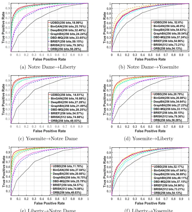
3.4 The ROC curves under different settings on Brown dataset when using
various unsupervised binary descriptors. Best viewed in color. . . 54
3.5 The matching results of Notre Dame, Yosemite and Liberty of UDBD
on Brown dataset, which includes three matched pairs and two
mis-matched pairs for each subset. . . 55
3.6 Precision-Recall curves of the proposed method and the baselines on
Cifar-10 dataset at 16, 32 and 64 bits. . . 56
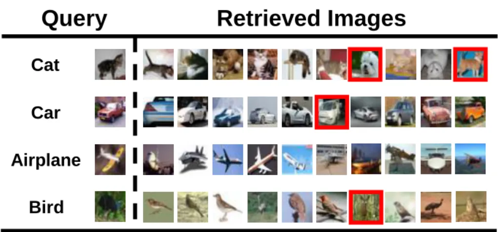
3.7 The top-10 retrieved images on Cifar-10 dataset by UDBD at the code
length of 64. The query images are selected from four categories: cat,
car, airplane and bird. Red rectangle indicates the wrong results. . . 57
3.8 Performances variations under different rotation angles on test
in-stances from GraphBit, DeepBit and UDBD. . . 59
3.9 Performance variations at varying code lengths with/without using
weak bit scheme. (a) FPR@95% on Brown: Notre Dame(ND)→Liberty
(Lib) and Liberty→Notre Dame; (b) Precision@Top 1 on Cifar-10. . . 60
3.10 Parameter sensitivity analysis ofγandβat various bit sizes on Cifar-10
dataset. . . 61
4.1 (a) Suppose that two data samples (red and green) from a benchmark
are projected into a two-dimensional feature space with the coordinates
of (x1, y1) and (x2, y2) and encoded by two bits subsequently, where
|x1| > |y1|, |x2| > |y2| and |x1 −x2| > |y1 −y2|. After the proposed
balanced rotation, the coordinates of two data points change to (xr1, yr1)
and (xr2, y2r) accordingly, where |xr1|= |yr1| and |xr2| = |y2r|. Obviously,
compared to the original features, the variances contained in the X
and Y axis can be balanced with such rotation strategy applied. That
indicates two dimensions of the rotated data points will have the same impact on the calculation of the Hamming distances when encoding them with the fixed number of bits; (b) The variance within each
LIST OF FIGURES xviii
4.2 The basic framework of UDVH-LSTM. The whole process consists of
three subsections: video feature extraction, unsupervised code learning and deep hash function learning, which are performed iteratively to
obtain the solution. . . 68
4.3 The basic framework of TSN. The only difference between UDVH-TSN and UDVH-LSTM is that they adopt LSTM and UDVH-TSN separately to evaluate the video representation. . . 70
4.4 The graph illustration of Algorithm 2. . . 77
4.5 The mAP@K curves at different bit sizes under UDVH-LSTM. . . 82
4.6 The Precision-Recall curves at 128 bits under UDVH-LSTM. . . 83
4.7 The Precision@100 curves at various bit sizes under UDVH-LSTM. . 83
4.8 Top-5 retrieval results when using SSTH and UDVH-LSTM at the code length of 128 bits. . . 85
4.9 The mAP@K curves at different bit sizes under UDVH-TSN. . . 86
4.10 The Precision-Recall curves at 128 bits under UDVH-TSN. . . 87
4.11 The Precision@100 curves at various bit sizes under UDVH-TSN. . . 87
4.12 Top-5 retrieval results when using SSTH and UDVH-TSN at the code length of 128 bits, where examples are randomly selected from the video datasets. The left column shows the query videos, the middle blocks and right blocks show the top-5 returned videos by SSTH and UDVH-TSN, respectively. Red rectangles indicate mistakes. . . 88
4.13 The variance distribution from FCVID at 128 bits under UDVH-TSN. 92 4.14 The mAP@5 variations when using CNN and TSN features separately in the image-based hashing methods, where the solid and dot lines represent the results on TSN and CNN features, respectively. . . 93
4.15 The mAP@5 variations when using CNN and TSN features separately in the video-based hashing methods, where the solid and dot lines represent the results on TSN and CNN features, respectively. . . 93
4.16 An example of cross-modality similarity search: text query image, in Google Images. . . 95
LIST OF FIGURES xix
5.1 The overview of our Self-Supervised Deep Multimodal Hashing. There
are three subsections in the training process: deep feature learning (left), deep hash function learning (middle) and regularized binary la-tent representation learning (right). Specifically, the regularized binary latent model consists of two loss terms: binary reconstruction loss and graph regularization loss. The yellow arrows indicate the deep feature learning. The blue arrows show the iterative directions when learning
deep hash functions with the guidance of the unified binary code B.
Better viewed in color. . . 99
5.2 The Precision-Recall curves at 128 bits on three datasets. . . 115
5.3 The top-5 retrieved results at 128 bits on Wiki dataset. . . 116
5.4 The top-5 retrieved results at 128 bits on MIRFlickr dataset. . . 117
5.5 The top-5 retrieved results at 128 bits on NUS-WIDE dataset. . . 118
5.6 mAP versus γ, β and λ at 64 bits on three datasets. . . 120
5.7 (a) Objective function values after each iteration (t) when solving the unified binary code at 128 bits; (b) Euclidean losses after every itera-tion (T) when learning the deep hash functions at 128 bits. . . 121
5.8 Time costs (in seconds) in optimizing one row of the unified binary code at 128 bits on three datasets when using BGD and One Entry [153] separately. . . 122
List of Acronyms
AGH Anchor Graph Hashing
ANN Approximate Nearest Neighbor
AVH Attention-based Video Hashing
BLSTM Binary Long Short Term Memory
BOLD Binary Online Learned Descriptor
BGD Binary Gradient Descend
BRE Binary Reconstructive Embedding
BRIEF Binary Robust Independent Elementary Features BRISK Binary Robust Invariant Scalable Keypoints
BQP Binary Quadratic Programming
CAH Correlation Autoencoder Hashing
CA-LBFL Context-Aware Local Binary Feature Learning C-CBFD Coupled Compact Binary Face Descriptor
CBIR Content-Based Image Retrieval
CCA Canonical Correlation Analysis
CDbin Compact Discriminative binary descriptors
CDQ Collective Deep Quantization
CMFH Collective Matrix Factorization Hashing
CMLA Cross-Modal correlation Learning with Adversarial samples
CMSSH Cross-Modal Similarity Sensitive Hashing
CNN Convolutional Neural Network
LIST OF FIGURES xxi
CNNH Convolutional Neural Network Hashing
CT Computed Tomographic
CVH Cross-View Hashing
CYC-DGH Cycle-Consistent Deep Generative Hashing DBD-MQ Deep Binary Descriptor with Multi-Quantization
DBRC Deep Binary Reconstruction
D-BRIEF Discriminative BRIEF
DCC Discrete Cyclic Coordinate Descent
DCMH Deep Cross-Modal Hashing
DDBC Discriminant Direction Binary Code
DLFH Discrete Latent Factor model based cross-modal Hashing
DGH Discrete Graph Hashing
DH Deep Hashing
DHH Deep Heterogeneous Hashing
DisCMH Discriminant Cross-Modal Hashing
DJSRH Deep Joint-Semantics Reconstructing Hashing
DNNH Deep Neural Network Hashing
DOAP Descriptors Optimized for Average Precision
DSADH Dual-Supervised Attention Network for Deep Hashing
DSH Deep Sketch Hashing
DVB Deep Variational Binaries
DVH Deep Video Hashing
DVSH Deep Visual-Semantic Hashing
EGDH Equally-Guided Discriminative Hashing
FCVID Fudan-Columbia Video Dataset
FPR@95% False Positive Rate at 95% true positive recall rate
LIST OF FIGURES xxii
GAN Generative Adversarial Network
GCH Graph Convolutional Hashing
GCN Graph Convolutional Network
GPU Graphics Processing Unit
HamH Harmonious Hashing
HER Hashing across Euclidean space and Riemannian manifold
HPatches Homography Patches
IMH Inter-Media Hashing
IMVH Iterative Multi-View Hashing
IsoH Isotropic Hashing
ITQ Iterative Quantization
ITQ+ Iterative Quantization Plus
JMVH Joint Multi-View Hashing
KAEs K-AutoEncoders
KD-tree K-Dimensional tree
KLSH Kernelized Locality Sensitive Hashing
KMH K-Means hashing
KNN K Nearest Neighbour
KSH Kernel Supervised Hashing
LBP Local Binary Pattern
LCMH Linear Cross-Modal Hashing
LDAHash Linear Discriminant Analysis Hashing
LDLP Local Diagonal Laplacian Pattern
LSH Locality Sensitive Hashing
LSSH Latent Semantic Sparse Hashing
LSTM Long Short-Term Memory
LIST OF FIGURES xxiii
MFH Multiple Feature Hashing
MGAH Multi-pathway Generative Adversarial Hashing
MLP Multi-Layer Perceptrons
MSAE Multi-modal Stacked Auto-Encoder
NDH Nonlinear Discrete Hashing
NN Nearest Neighbor
NP Non-deterministic Polynomial
NPH Neighborhood Preserving Hashing
NSH Nonlinear Structural Hashing
ORB Oriented fast and Rotated BRIEF
OKH Online Kernel-based Hashing
OSH Online Sketching Hashing
PCA Principal Component Analysis
PR curve Precision-Recall curve
Precision@KPrecision at top-K retrieved candidates
QCH Quantized Correlation Hashing
RFDH Robust and Flexible Discrete Hashing
RNN Recurrent Neural Network
RPN Region Proposal Network
RFDH Robust and Flexible Discrete Hashing
RI-LBD Rotation-Invariant Local Binary Descriptor
SAE Semantic Auto-Encoder
SBIR Sketch-Based Image Retrieval
SCM Semantic Correlation Maximization
SCMFH Supervised Collective Matrix Factorization Hashing
SDCH Semantic Deep Cross-modal Hashing
LIST OF FIGURES xxiv
SePH Semantics-Preserving Hashing
SGD Stochastic Gradient Descent
SIFT Scale-Invariant Feature Transform
SLBFLE Simultaneous Local Binary Feature Learning and Encoding
SMVH Stochastic Multi-view Hashing
SpH Spherical Hashing
SP SPectral hashing
SPDTH Similarity-Preserving Deep Temporal Hashing
SRBD Superpixel Region Binary Descriptor
SSDMH Self-Supervised Deep Multimodal Hashing
SSTH Self-Supervised Temporal Hashing
SSE Semantic Similarity Embedding
SSVH Self-Supervised Video Hashing
SUBIC SUpervised structured BInary Code Submod Submodular video hashing
SURF Speeded Up Robust Features
SVM Support Vector Machine
TDH Triplet-based Deep Hashing
TSN Temporal Segment Network
TVDB Textual-Visual Deep Binaries
UDBD Unsupervised Deep Binary Descriptor
UDCH-VLR
Unsupervised Deep Cross-modal Hashing with Virtual Label Regres-sion
UDCMH Unsupervised Deep Cross-Modal Hashing
UDVH Unsupervised Deep Video Hashing
List of Algorithms
1 Unsupervised Deep Binary Descriptor . . . 50
2 Unsupervised Deep Video Hashing . . . 76
3 Self-Supervised Deep Multimodal Hashing . . . 108
Chapter 1
Introduction and Background
Theory
1.1
Research Background
Living in the Internet era of big data, the explosive amount of data, which varies in diverse forms like image, text, audio, and video, has become extremely challeng-ing more than ever for the existchalleng-ing multimedia search engines and recommendation systems. According to recent public statistics from two popular social media
web-sites, the average number of photos being shared every day on Flickr1 is more than
1 million. In comparison, over 500 hours of videos are uploaded per minute by the
active users onYoutube2. To tackle such overwhelming data sources, how to perform
accurate and efficient content-based similarity retrieval, which is a core technology of the current multimedia systems, has aroused extensive attention from both industry and academia.
The similarity retrieval problem, also known as Nearest Neighbor (NN) search, can be described as a search process of finding the most relevant semantic (similar) candidates from a large gallery set for a given query sample [149, 165, 193].
Particu-larly, given a query feature vector xq ∈Rd, a gallery set consists ofn feature vectors
X= [xi]ni=1 ∈Rd
×n, d is the dimensionality, the nearest neighbor search problem can
be formulated as: N N(xq) = arg min x∈X dist(xq, x), (1.1) 1https://expandedramblings.com/index.php/flickr-stats/ 2 https://www.tubefilter.com/2019/05/07/number-hours-video-uploaded-to-youtube-per-minute/ 1
1.1. RESEARCH BACKGROUND 2 Feature Extraction Encoding Feature Extraction Encoding Gallery Feature Vectors Query Feature Vector Retrieval Gallery Query Relevant Images
Content-Based Image Retrieval
Figure 1.1: The general procedure of CBIR.
wheredist(.) represents a specific distance metric (e.g., Euclidean distance) that
de-termines the closest candidates to xq in the feature space. To further clarify the
similarity retrieval process, a simple flowchart of the general content-based image re-trieval (CBIR) [165] is presented in Fig. 1.1, which could be easily extended to other related tasks involving different data types. In CBIR, images are firstly represented with various feature vectors and then encoded into alternative representations follow-ing certain patterns (i.e., encodfollow-ing function). Here, the encodfollow-ing function, which is also the learning objective in most search frameworks, should be carefully designed to obtain better performance in the upcoming retrieval tasks. Then, the gallery and query data are pre-computed by the learned encoding function and their encoded feature vectors are measured under a distance metric. By sorting those distances in an ascending order, the candidates from the gallery with the smallest distances are returned as the relevant (i.e., similar) neighbors to one specific query. Generally speaking, the search efficiency depends on the computational complexity of the re-trieval phase. At the same time, the search accuracy is usually determined by the proper design of the encoding mechanism when using fixed feature extractor [7, 193]. The earliest works in the research of similarity retrieval perform the exhaus-tive/exact Nearest Neighbor (NN) search in the retrieval process. However, such a search strategy (i.e., linear scan) shows weakness in tackling large-scale datasets
1.1. RESEARCH BACKGROUND 3
with numerous samples in practical applications. Later on, some tree-based search schemes are proposed to subdivide the feature space for data samples via employing various tree structures for fast search. Two representative methods are K-Dimensional tree (KD-tree) and Randomized KD-tree [46, 132], which indexes the data for quick query responses. However, these methods cannot handle the high-dimensional cases, known as the curse of dimensionality, where the computational costs grow exponen-tially along with the increasing dimension, thus making it less favorable in large-scale retrieval applications [149, 193].
Consequently, Approximate Nearest Neighbor (ANN) search has been developed rapidly, where the hashing-based approaches draw considerable attention in this research field to overcome the limitations via conducting efficient retrieval in low-dimensional (i.e., compact) Hamming space [78]. The core idea of hashing is to rep-resent the high-dimensional real-valued original data with a series of compact binary codes while preserving the semantics as much as possible during the code learning, thus accelerating the retrieval process without compromising the accuracy [193, 194].
Two advantages of hashing algorithms3 are presented as follows:
• By representing data with compact binary code, it enables efficient similarity
retrieval by only conducting bitwise operation when computing the Hamming distance between data samples;
• It reduces the memory space to the maximum extent in storing the massive
features and conducting the large-scale retrieval due to the nature of compact binary code [51, 165, 177, 193, 197].
These unique characteristics make hashing extremely competitive in conducting
large-scale visual-related similarity search tasks. In this thesis, we will focus on
learning compact binary representation via a hashing algorithm for the large-scale multimedia similarity search tasks. Particularly, we propose several new hashing frameworks and apply them in three major applications like local binary descriptors
for patch-level4 matching and retrieval (Chapter 3), video-to-video retrieval (Chapter
4) and cross-modality retrieval (Chapter 5). The proposed methods cover various forms of the similarity search tasks, from single-modality to cross-modality, and also enable to tackle different forms of multimedia data, e.g., image, text, and video [50, 186].
3Hashing algorithm and hashing technique are used interchangeably in this thesis.
4Patch (i.e., small image) with small size (e.g., 64×64, 32×32) is generated as the composition
1.2. FUNDAMENTAL THEORY OF HASHING TECHNIQUE 4
In the following subsections, we provide further insights on the fundamental theory of the hashing algorithm first and briefly present the motivations when proposing those novel methods. Then we summarize the contributions for each chapter. Finally, the organization of this thesis is given.
1.2
Fundamental Theory of Hashing Technique
Given a data sample represented by a feature vector x ∈ Rd, the ultimate goal of
hashing technique (i.e., learn to hash) is to design an optimal hash function h(.)
that projects x from the original high-dimensional space into compact binary space
b ∈ {−1,1}p (
Rd → Rp and d >> p), while keeping its true nearest neighbors as
closer as possible in the Hamming space [193, 194, 197]. In other words, the similar data samples in the original feature space should be represented with similar (low Hamming distance) binary codes, thus improving the retrieval efficiency dramatically with decent accuracy.
To achieve that learning goal, several crucial problems should be considered when designing a robust hashing framework. In this thesis, we address them concisely from five different aspects: hash function, objective function construction, optimization strategy, fast similarity search with hash code, and evaluation metrics.
1.2.1
Hash Function
As discussed above, hash function plays a crucial role in determining the retrieval accuracy in the applications of hashing technique and the code generalization effi-ciency [194]. Notably, we can formulate the general hashing process as follow:
h(x)→b, (1.2)
where the hash function h(.) can be summarized into two main types: linear and
nonlinear functions. An example of the generalized linear hash function is given as below:
sign(Wx+y)→b, (1.3)
where W∈Rp×d and y ∈
Rp represent the linear projection matrix and bias vector,
respectively. Hard thresholding function sign(x) equals 1 if x ≥ 0, otherwise −1.
However, in real applications, linear hash function usually suffers from less discrimi-native power though simplicity itself [111].
1.2. FUNDAMENTAL THEORY OF HASHING TECHNIQUE 5
h(x) = 1
h(x) = 0
Linear Nonlinear Feature SpaceFigure 1.2: An example of linear and nonlinear models. Given two different data distributions (triangle and parallelogram), the nonlinear model can better fit the complicated data distributions than the linear one.
To overcome the discussed limitation of the linear hash function, nonlinear hash functions have been widely developed in recent studies, where kernel, spherical func-tion, or boosting model can be applied to the original feature before the binarization. Compared to the linear hash function, such nonlinear operation enables to enhance the feature expressive ability, which is more compatible with the real data collected from complex real-world scenarios [23]. Fig. 1.2 gives a simple example in such a case. Without loss of generality, the widely-used kernel-based hash function is presented as below:
sign(X i
Wiφ(ci, x) +y)→b, (1.4)
whereci denotes the randomly-sampled data point or cluster center from the dataset.
φ(.) is the kernel function [91] andWi represents the weight matrix.
With the recent development of deep learning technologies, deep neural networks have been widely incorporated into the hashing frameworks, which can also be treated as an advanced form of nonlinear hash functions with various activation functions [23, 43,94,219]. In this thesis, deep networks are also adopted as hash functions to improve the performance of our methods.
1.2. FUNDAMENTAL THEORY OF HASHING TECHNIQUE 6
1.2.2
Objective Function Construction
Constructing a proper objective (i.e., loss) function is the most crucial factor in obtaining better retrieval performance for a hashing framework. Generally, most existing methods build their loss functions with two essential elements: learning the hash function while keeping the similarity consistency between feature spaces at the same time [194]. For the hash function learning part, one of the most commonly
adopted solutions is to minimize the loss between hash code b and hash function
h(x), which can be generalized as a loss term below:
minkb−h(x)k2
F, (1.5)
where Frobenius norm (i.e.,k.kF) is used here as an example, and the distance metrics
might vary in different methods. The hash functionh(x) can be in the forms of linear
or nonlinear, as discussed in the previous section. The underlying meaning of Eq. (1.5) is to bridge the original feature space and compact Hamming space via learning the hash function, which is also described as a projection (i.e., mapping) procedure in most related works [51, 193].
Regarding the similarity-preserving criterion, the core concept focuses on keeping the consistency between the original and binary spaces for the similar data samples during the learning process such that they are more likely to be represented by similar hash codes. In most existing hashing works, the similarity-preserving criterion can be achieved by including pairwise-, multiwise- or quantization-based solutions in the objective function [194, 197], where a simple example is provided for each solution to clarify the problem. Particularly, in the pairwise similarity-preserving criterion, the distances or similarities of a pair of data samples are aligned in the loss term. One of the most representative works is SPectral hashing (SP) [211], where the similarity-preserving term is formulated as:
minX i,j sijdij = X i,j sijkbi−bjk2. (1.6)
Here, the similaritysij is calculated ase−
kxi−xjk2
σ2 for a pair of data pointsx
i andxj. Eq. (1.6) measures the average Hamming distance between similar neighbors [211]. While in the multiwise similarity-preserving criterion, the distances or similarities of more than one pair of data points are considered, where the triplet loss is widely
1.2. FUNDAMENTAL THEORY OF HASHING TECHNIQUE 7
and their binary codes as b, b+, b−, x+ is more similar to x than x−, the triplet loss
term is written as follow:
max(1− kb−b−k1+kb−b+k1,0). (1.7)
According to Eq. (1.7), the loss term would be penalized when b− is more (or
equally) similar to b than b+, thus preserving the similarity structure during the
optimization. In the quantization-based methods, the reconstruction loss function is generally employed to find the optimal approximations of original data points in the compact Hamming space. A good example of this case is Iterative Quantization (ITQ) [51] and its objective function can be formulated as below:
min B,RkB−R TVk2 F =kB−R TPTXk2 F, (1.8)
where V = PTX denotes the projected feature after Principal Component Analysis
(PCA) [213] on the centralized input X. To be specific, ITQ aims at exploiting
an orthogonal rotation matrix R via iterative optimization such that similar data
points could be aligned properly in the binary space [51]. The performance from these quantization-based methods significantly relies on the feature distribution (e.g., zero-centered) and projection quality.
In the above discussions, we have presented two essential elements of constructing
a hashing objective function. It worth noting that the solutions above could be
expanded as different forms but not limited to merely Eq. (1.5), (1.6), (1.7) and (1.8) [194]. Many extra problem-oriented components (e.g., regularization terms or restrict conditions) could be added to the loss function for better similarity search quality.
1.2.3
Optimization Strategy
Due to the discrete constraints introduced by the sign function, it is exceptionally
challenging to optimize the non-convex objective functions (i.e., mixed-binary-integer optimization problem) directly in most hashing methods [194, 197]. Subsequently, various discrete optimization strategies have been proposed in previous works, and they can be roughly categorized into three mainstream types as follows.
1.2.3.1 Continuous Relaxation
During the optimization, the binary constraints are relaxed to continuous variables
1.2. FUNDAMENTAL THEORY OF HASHING TECHNIQUE 8
x → 1
1+e−x ∈ (0,1) and tanh : x →
ex−e−x
ex+e−x ∈ (−1,1)) [117, 166] or even discarding
the sign function (i.e., sign(x) ≈ x) [118]. The purpose of performing continuous
relaxation is to make the objective function differentiable such that standard gradient-based optimization schemes can be applied. However, the direct optimization over the relaxed variable cannot guarantee the optimal solution because of the gaps between approximated and real hash codes.
1.2.3.2 Alternative Optimization
In this learning paradigm, the discrete optimization procedure is decomposed into two distinct stages, namely, learn hash codes first and build hash functions afterward based on the learned codes (i.e., two-stage optimization) [105, 238]. In other words, there is no need to update the hash function during each iteration of code learning, which reduces the computational costs to some extent. For example, in [238], the binary codes are generated via exploiting the eigenvalues in a relaxed version of the Laplacian graph and then train the Support Vector Machine (SVM) classifiers as hash functions by using the learned binary codes as class labels. However, such a learning strategy usually leads to locally optimal solutions because of the separate optimization steps.
1.2.3.3 Coordinate Descent
Instead of applying relaxation strategy, the binary constraints remain unchanged dur-ing the optimization process, and the objective function is optimized iteratively via flipping each entry within hash code sequentially, which indicates that a single bit is learned based on the rest fixed bits in one binary vector [153]. However, the ob-jective function is usually required to follow specific patterns (e.g., Binary Quadratic Programming problem [228]) or adopt a proper initialization strategy to make the coordinate-descent optimization tractable. More worriedly, the bit-by-bit optimiza-tion scheme is extremely low-efficient, which is also addressed in Chapter 5.
Generally speaking, the presented optimization strategies are all double-edged
swords. Nevertheless, they provide flexible solutions when tackling such discrete
optimization problems in hashing applications. Some of those strategies are also adopted in our works, which will be detailed in the following chapters.
1.2. FUNDAMENTAL THEORY OF HASHING TECHNIQUE 9 Hash Function 1 0 1 0 1 1 0 1 1 0 1 0 1 1 0 1 1 1 0 1 1 0 1 1 Dh=1 1 0 1 0 0 1 0 1 1 1 1 0 1 1 0 1
……
Dh=2 Dh=6 Dh=1 Gallery Query Ranked ResultsFigure 1.3: The search procedure of hash code ranking. The ranked results are
obtained based on the Hamming distances (Dh) in an ascending order.
1.2.4
Fast Similarity Search with Hash Code
As long as we can obtain binary codes for the data from the proposed hash function, efficient nearest neighbor search can be conducted by using one of the following search strategies: hash code ranking and hash table lookup [194, 197].
1.2.4.1 Hash Code Ranking
As the most straightforward hashing-based search strategy, in the hash code rank-ing, the Hamming distances between the binary codes of query and gallery data are exhaustively calculated via bitwise XOR operation and then sorted in ascending order, where the candidates with smallest Hamming distances are returned as the nearest neighbors to that query. This search strategy exhibits one main advantage of using hash codes rather than real-valued representations, where the Hamming dis-tance between hash codes can be computed efficiently with much lower computational costs, comparing to that under other distance metrics (e.g., Euclidean distance) in the original feature space [194]. Besides, hash code ranking adopts an exhaustive search strategy to provide coarse-level retrieved candidates for query data and more re-ranking techniques can be further applied for the fine-grained retrieval results. A
1.2. FUNDAMENTAL THEORY OF HASHING TECHNIQUE 10 x1, x4, x5 x2 x3, x6 ……… xn 0110 1110 0100 1111 Hash Table Query 0110 h(.)
(a) Single table lookup
x2, x4 x8 x3, x6 ……… xn Hash Table 1 Query hM(.) x2 x3,x9 x1, x10 ……… x5 Hash Table M h1(.)
………
(b) Multiple table lookup
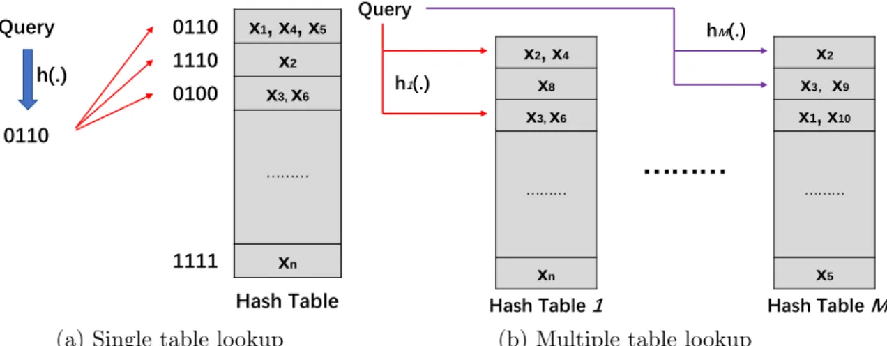
Figure 1.4: (a) 4-bit hash code is used as an example. The returned items would be
x1, x4, x5, x2, x3 and x6 if the Hamming radius is 1; (b) M(M >1) hash tables are
constructed in the multiple table lookup and the neighbor search is conducted across these tables afterward.
simple example of the hash code ranking is presented in Fig. 1.3 and it has been widely adopted to evaluate the system performance of our methods and the state-of-the-arts.
1.2.4.2 Hash Table Lookup
Theoretically, the search process of the hash table (i.e., hash map) lookup is more complicated than the hash code ranking. Precisely, the hash table consists of multiple buckets, where each bucket is indexed by unique hash code and assigned with at least one item (i.e., data sample) from the gallery under the perfect condition. One fundamental principle in constructing such a hash table is maximizing the probability of similar items being stored in the same bucket and vice versa. It speeds up the search process via reducing the frequency of distance computations in the inverse lookup when given a query data [22, 194].
There are two different types: single table and multiple tables, in the hash table
lookup. In single table lookup, all gallery items (e.g., x1, x2, ..., xn in Fig. 1.4(a))
are placed in one table and the query needs to visit more buckets to guarantee the
retrieval accuracy. In multiple tables lookup, a bunch of tables (e.g.,M in Fig. 1.4(b))
are constructed to store multiple copies of those gallery items. By placing the item copies in multiple hash tables, it obtains satisfactory performance by improving the possible hit number of each relevant item though relatively high space costs. Fig. 1.4 briefly presents the hash table indexing procedures. The hash table lookup is
1.2. FUNDAMENTAL THEORY OF HASHING TECHNIQUE 11
widely employed to evaluate the retrieval performance of those LSH-based methods and more details on hash table lookup can be found in [160, 194, 197, 211].
1.2.5
Evaluation Metrics
Several popular performance evaluation metrics used to measure the search quality are elaborated in this section, including Precision@K, Mean Average Precision, Precision-Recall Curve and Receiver Operating Characteristic Curve.
1.2.5.1 Precision@K
Precision at top-K retrieved candidates (Precision@K) is one of the most fundamental performance evaluation metrics in large-scale information retrieval. In this thesis, Precision@K can be computed as:
P recison@K = |{Relevant Data}
T{
T op K Retrieved Data}|
K , (1.9)
where |.| denotes the size of the common subset. This metric has been used in the
experiments of Chapter 3, Chapter 4 and Chapter 5. 1.2.5.2 Mean Average Precision
In the information retrieval, mean Average Precision (mAP)5 is a crucial retrieval
performance metric. To calculate the mAP score, the average precision of each query should be computed first during the retrieval. To be specific, the average precision on the retrieved results for one query is calculated as:
Average P recison=
PNc
k=1(P recision@k×Rel(k))
|{relevant data}| . (1.10)
where Nc denotes the retrieved candidates number. Rel(k) refers to an indicator
function, which equals 1 if the relevant item to the query is retrieved at rank k and
otherwise 0 [185]. Therefore, the mAP value for all the queries during the retrieval can be calculated as below:
mAP =
PNq
i=1Average P recision(qi)
Nq
, (1.11)
where Nq is the queries number. This metric has been used in the experiments of
Chapter 3, Chapter 4 and Chapter 5.
1.2. FUNDAMENTAL THEORY OF HASHING TECHNIQUE 12
1.2.5.3 Precision-Recall Curve
In information retrieval, precision is a measure of result relevancy, while recall is a measure of how many genuinely relevant results are returned. The Precision-Recall (PR) curve shows the tradeoff between precision and recall for different thresholds. A high area under the curve represents both high recall and high precision, where high precision relates to a low false-positive rate, and high recall refers to a flat false-negative rate. High scores of both metrics show that the classifier is returning accurate results (high precision), as well as returning a majority of all positive results (high recall).
Particularly, precision is defined as the number of true positives (Tp) over the
number of true positives plus the number of false positives (Fp), which is formulated
as:
P recision= Tp
Tp+Fp
. (1.12)
Recall is defined as the number of true positives (Tp) over the number of true
positives plus the number of false negatives (Fn), which is computed as:
Recall = Tp
Tp+Fn
. (1.13)
This metric has been used in the experiments of Chapter 3, Chapter 4 and Chapter 5.
1.2.5.4 Receiver Operating Characteristic Curve
Receiver Operating Characteristic (ROC) curve is determined by True Positive Rate (TPR) and False Positive Rate (FPR). To be specific, TPR is defined as the number
of true positives (Tp) over the number of true positives (Tp) plus the number of false
negatives (Fn), which is formulated as:
T P R= Tp
Tp+Fn
. (1.14)
FPR is defined as the number of false positives (Fp) over the number of true
negatives (Tn) plus the number of false positives (Fp), which is calculated as:
F P R= Fp
Tn+Fp
. (1.15)
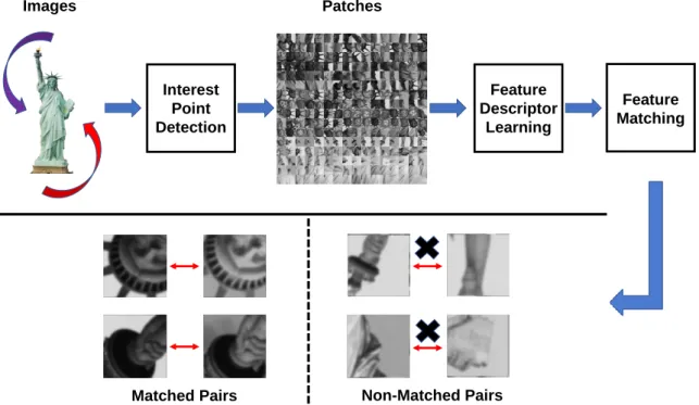
1.3. RESEARCH PROBLEMS AND CHALLENGES 13 Feature Descriptor Learning Feature Matching Interest Point Detection
Matched Pairs Non-Matched Pairs
Images Patches
Figure 1.5: The work pipeline of traditional image matching using local feature de-scriptor, which consists of three major steps: interest point detection, feature descrip-tor learning and feature matching. The feature learning and matching processes are conducted at the patch level. The input images might be photographed from different views or even processed with various affine transformations.
In the next section, we will present the concrete research problems and challenges in designing the hashing algorithms for various applications in this thesis.
1.3
Research Problems and Challenges
Although considerable success has been achieved by the modern hashing methods in a wide range of various similarity search tasks, there are still several limitations that need to be addressed for better system performance. In this thesis, we mainly focus on three popular hashing applications: image matching/retrieval with the local binary descriptor, video hashing, and cross-modality hashing, where the existing challenges that motivate our works in these applications are elaborated.
1.3.1
Local Binary Descriptor
Fig. 1.5 shows the traditional image matching process by using a local feature de-scriptor. To be specific, it first generates local patch sets for each image by the in-terest point detectors, such as Scale Invariant Transform Invariant (SIFT) [121] and
1.3. RESEARCH PROBLEMS AND CHALLENGES 14
Hessian-Affine [129], and learns the corresponding local feature descriptor for each patch. Then the feature matching can be conducted by measuring the distance (e.g., Euclidean distance) between those descriptors. Especially, matching can be treated as a particular case of retrieval, where only one exact candidate is returned for the query in the matching process. The fundamental principle of designing local feature descriptors is that the descriptor should be robust against various geometric transfor-mations like rotation, translation, and scaling, etc. [97,121]. In the earlier works, they mainly focus on learning the real-valued feature descriptors for the matching process. Hundreds of interest points per image would be selected and the high-dimensional feature vectors for each patch are usually required, which leads to high computation complexity and memory costs in the upcoming matching process. Consequently, the binary descriptor has drawn extensive attention to accelerate the matching process while consuming low computing resources. In this thesis, we discuss several limita-tions of the existing binary descriptors below.
• Earlier binary descriptors (e.g., Binary Robust Independent Elementary
Fea-tures (BRIEF) [17], Binary Robust Invariant Scalable Keypoints (BRISK) [97]) generally adopt shallow handcrafted sampling patterns and perform pairwise intensity comparisons to generate the feature descriptors [231]. For example, in BRIEF, a bunch of specific location pairs are selected from the smoothened image patch and pixel-level intensity comparison is conducted between each pair [17]. However, such handcrafted descriptors are extremely vulnerable to the distortions/transformations, which yields unstable performance when tack-ling large-scale visual recognition tasks [182, 183, 231].
• The learning-based binary descriptor is becoming a popular research topic for its
desirable performance against those handcrafted ones. Most previous methods adopt hashing ideas and pay intense attention to novel discrete optimization strategies, however, the basic principle in designing local feature descriptors, anti-geometric transformation, is not considered during the optimization [97, 183]. Moreover, most learning paradigms fail to preserve the manifold structure during the discrete optimization, which makes binary descriptor less effective in the large-scale nearest neighbor search tasks [56, 107, 153].
• Traditional binary descriptors measure the similarity between database and
query via performing exhaustive Hamming distance calculations in the testing phase, which is more likely to return many candidates with equal Hamming
1.3. RESEARCH PROBLEMS AND CHALLENGES 15
Feature
Fusion Hashing Retrieval
Video Gallery Hashing Relevant Videos Feature Extraction
…
…
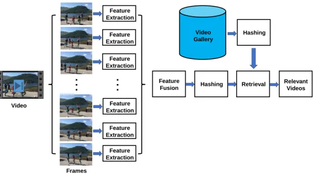
Video Frames Feature Extraction Feature Extraction Feature Extraction Feature Extraction Feature ExtractionFigure 1.6: The general pipeline of video retrieval.
distances to one specific query compared to using the real-valued feature de-scriptors [120]. However, the ultimate goal of the feature matching is to find one exact candidate (with the lowest Hamming distance) to a specific query rather than returning a bunch of ambiguous options (with equal minimum Hamming distance) in the general retrieval process.
Those defects give rise to the less favorable performance from the previous binary descriptors and should be carefully addressed in the descriptor learning to improve the matching accuracy.
1.3.2
Video Hashing
Fig. 1.6 presents the general pipeline of video retrieval based on the hashing algo-rithm. Compared with images, videos, which can be treated as more complicated 3D signals, are more difficult to be hashed because of variable lengths and tremendous redundancies. To tackle those issues, video is firstly represented as a certain number of consecutive keyframes prior to employing various hashing algorithms, as shown in Fig. 1.6 [243]. However, two major limitations in previous works impede their performance in large-scale video retrieval, which are presented as follows:
• In earlier video hashing methods [28,38,172], they generally wrap the
1.3. RESEARCH PROBLEMS AND CHALLENGES 16
fusion strategies, and then apply the binarization tactics from image hash-ing [51, 211] on the concentrated feature directly. Some of them even perform image hashing on each frame independently and generate video hash code by thresholding the average value of all frame-level binary codes [24]. However, such learning paradigms degrade the quality of video hash code significantly because of the improper hashing mechanisms and the ignorance of the video’s temporal nature [109, 197, 200, 225].
• As revealed in recent studies on video representation learning, it is more likely
to obtain better video features via incorporating the frame-level spatial infor-mation with the temporal inforinfor-mation of a video sequence, thus improving the system performance in various vision tasks [175, 226, 235]. Currently, two main-stream ways to obtain such video feature are presented as follows: 1) feeding the sparsely-sampled frame-level image features from a video clip into Recur-rent Neural Network (RNN) or Long-Short Term Memory (LSTM) [73] in order to explore the temporal nature and then aggregating into the global video-level feature [109, 197, 217]; 2) fusing the spatial and temporal features (e.g., optical flow) from the two-stream networks to generate the unified video representation via various pooling schemes [200]. However, those operations usually make the synthetic video feature with more scattered (less correlated) distribution and unbalanced dimensions compared to the pure image feature [86, 175]. When projecting these video features into the low-dimensional compact space before the binarization step, the data variances on projected dimensions tend to be large (i.e., unbalanced) [35, 57, 58]. Especially for the fixed bit quantization, this imbalanced projection will degrade the performance of the generated hash codes because each dimension will be treated equivalently and allocated with the same number of bits (e.g., 1 bit in most existing works) in the quantization step afterward. It is unable to achieve effective hash codes for video retrieval due to such an unfair bit assignment scheme.
1.3.3
Cross-Modality Hashing
Fig. 1.7 depicts the general process of cross-modality hashing, where the pairs of image and text are utilized in the training phase and the cross-modal retrieval tasks:
image→text and text→image6, are performed afterward. Compared with the
single-6Image
text is used as an example here. Other data types (e.g., audio and video) can also be
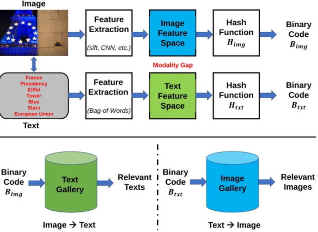
1.3. RESEARCH PROBLEMS AND CHALLENGES 17 France Presidency Eiffel Tower Blue Stars European Union Feature Extraction (sift, CNN, etc.) Feature Extraction (Bag-of-Words) Image Feature Space Hash Function 𝑯𝒊𝒎𝒈 Text Feature Space Hash Function 𝑯𝒕𝒙𝒕 Binary Code 𝑩𝒊𝒎𝒈 Binary Code 𝑩𝒕𝒙𝒕 Modality Gap Image Text Text Gallery Binary Code 𝑩𝒊𝒎𝒈 Relevant Texts Binary Code 𝑩𝒕𝒙𝒕 Image Gallery Relevant Images
Image →Text Text →Image
Figure 1.7: The general workflow of cross-modality retrieval. Two cross-modal
re-trieval tasks: image→text and text→image, are used as examples.
modality retrieval (e.g., video-to-video retrieval discussed in the previous section), the data instances are not in the same feature space when conducting the cross-modality similarity search. One of the main challenges in this research field is how to tackle the semantic gaps within different modalities (i.e., modality gap) properly. Many types of research have been devoted to handling this problem, however, some defects from these methods become the hard barriers of retrieval performance gains.
• Most existing methods, both in unsupervised [35, 170, 190] and supervised [10,
108, 180, 223] manners, concentrate on exploring a common latent space for the data from various modalities during the training process such that the heterogeneity among modalities can be minimized [35, 108]. For instance, as a classical work in the common latent space learning, matrix factorization is adopted in [34] to model the relations among different modalities. Specifically, a two-stage learning strategy is applied in learning unified binary code, where the original features of data points from different modalities are first projected into a real-valued common latent space, and then the latent space is quantized
1.3. RESEARCH PROBLEMS AND CHALLENGES 18
to obtain the binary code. Recently, deep learning technology has been widely incorporated in the cross-media hashing, which improves retrieval performance with better feature representation and nonlinearity modeling ability [210]. How-ever, most of those deep-based methods still employ a two-step scheme in the code learning following [34], where large quantization errors exist in the bina-rization step [189]. That is to say, the two-stage learning paradigm yields large quantization errors, and such errors will be further magnified after the itera-tive code learning, thus leading to suboptimal results because of the bad code quality.
• Moreover, most previous works focus on learning the unified representation for
the multimodal inputs. However, neighborhood structures from the original feature space are not well preserved, thus compromising the retrieval perfor-mance significantly because of less discriminative code. In another word, only instances within data pairs (e.g., a pair of image and its description) are repre-sented with the same binary code in the simple common latent space learning. While the positions between data pairs cannot be guaranteed in the binary space after the projection. Compared to unsupervised methods, supervised cross-modal hashing addresses this issue with the aid of dedicated prior knowl-edge (e.g., semantic labels, similarity matrix) [199]. Nevertheless, such similar-ity preservation is usually performed on approximated (i.e., real-valued) hash codes without any restrictions on binary codes in the training process, where the gap between real-valued and binary spaces makes that operation less effec-tive [108, 126, 202, 204, 223].
Based on the discussions above, the retrieval performance would be profoundly affected by those drawbacks, thus preventing the existing methods from massive de-ployment in real-world cross-media similarity search applications.
In this section, we have discussed the significant research challenges concisely in various hashing-based applications. To handle those problems above, several novel solutions are proposed for those applications separately, which will be further detailed in the main chapters. In the next subsections, we briefly summarize the contributions of each work and provide the chapter outlines correspondingly.